The Odd Exponentiated Half-Logistic Exponential Distribution: Estimation Methods and Application to Engineering Data

Abstract

In this paper, we studied the problem of estimating the odd exponentiated half-logistic exponential (OEHLE) parameters using several frequentist estimation methods. Parameter estimation provides a guideline for choosing the best method of estimation for the model parameters, which would be very important for reliability engineers and applied statisticians. We considered eight estimation methods, called maximum likelihood, maximum product of spacing, least squares, Cramér–von Mises, weighted least squares, percentiles, Anderson–Darling, and right-tail Anderson–Darling for estimating its parameters. The finite sample properties of the parameter estimates are discussed using Monte Carlo simulations. In order to obtain the ordering performance of these estimators, we considered the partial and overall ranks of different estimation methods for all parameter combinations. The results illustrate that all classical estimators perform very well and their performance ordering, based on overall ranks, from best to worst, is the maximum product of spacing, maximum likelihood, Anderson–Darling, percentiles, weighted least squares, least squares, right-tail Anderson–Darling, and Cramér–von-Mises estimators for all the studied cases. Finally, the practical importance of the OEHLE model was illustrated by analysing a real data set, proving that the OEHLE distribution can perform better than some well known existing extensions of the exponential distribution.

1. Introduction

The exponential (E) distribution with its simple form, lack of memory property and only a constant hazard rate shape, has attracted many authors to develop more flexible and extended forms of the E distribution. These extended forms are capable of modelling real data sets with decreasing, increasing, bathtub, decreasing–increasing, and unimodal failure rates which are very common in several applied areas such as reliability, medicine, and engineering, among others. Some notable extended forms of the E model are called, the exponentiated-E [1], Harris extended-E [2], beta-E [3], transmuted generalised-E [4], alpha power-E [5,6], Kumaraswamy transmuted-E [7], modified-E [8], Marshall–Olkin logistic-E [9], Burr-X exponentiated-E [10], Marshall–Olkin alpha power-E [11], odd log-logistic Lindley-E [12], and extended odd Weibull-E [13], among many others.

Afify et al. [14] proposed and studied the three-parameter odd exponentiated half-logistic-E (OEHLE) distribution which can exhibit constant, increasing, decreasing, or bathtub hazard rate shapes. Its probability density function (PDF) can be reversed-J shaped, symmetric, right-skewed and left-skewed. They investigated some of its fundamental properties such as quantile and generating functions, mean residual life, mean inactivity time, moments, and some characterisations. The OEHLE is applied to two engineering data sets, including strengths of 1.5 cm glass fibres data and the breaking stress of carbon fibres data. They proved that it provides better fits to both data sets than the exponentiated Weibull, Kumaraswamy transmuted-E, Kumaraswamy-E, beta-E, gamma, transmuted generalised-E, exponentiated-E, alpha power-E, and E distributions.

The OEHLE is constructed based on the odd exponentiated half-logistic-G (OEHL-G) class proposed by [15].

The cumulative distribution function (CDF) of the OEHL-G family takes the form:

$$F\left(x;\delta ,\gamma ,\mathit{\phi }\right)={\left[\frac{1-{\mathrm{e}}^{-\frac{\gamma G\left(x;\mathit{\phi }\right)}{1-G\left(x;\mathit{\phi }\right)}}}{1+{\mathrm{e}}^{-\frac{\gamma G\left(x;\mathit{\phi }\right)}{1-G\left(x;\mathit{\phi }\right)}}}\right]}^{\delta }, \delta ,\gamma >0, x\in \Re .$$

(1)

The PDF of the OEHL-G class reduces to:

$$f\left(x;\delta ,\gamma ,\mathit{\phi }\right)=2\gamma \delta g\left(x;\mathit{\phi }\right)\frac{e^{-\frac{\gamma G\left(x;\mathit{\phi }\right)}{1-G\left(x;\mathit{\phi }\right)}}{\left[1-{\mathrm{e}}^{-\frac{\gamma G\left(x;\mathit{\phi }\right)}{1-G\left(x;\mathit{\phi }\right)}}\right]}^{\delta -1}}{{\left[1-G\left(x;\mathit{\phi }\right)\right]}^2{\left[1+{\mathrm{e}}^{-\frac{\gamma G\left(x;\mathit{\phi }\right)}{1-G\left(x;\mathit{\phi }\right)}}\right]}^{\delta +1}}, \delta ,\gamma >0, x\in \Re ,$$

(2)

where $G\left(x;\mathit{\phi }\right)$ and $g\left(x;\mathit{\phi }\right)$ are the respective baseline CDF and PDF with $\mathit{\phi }$ (a parameter vector) and shape parameters, $\delta$ and $\gamma$, which give more flexibility to the generated model to accommodate all important hazard rate function (HRF) forms.

The CDF and PDF of the OEHLE distribution (Afify et al. [14]) are given by

$$F\left(x;\delta ,\gamma ,\theta \right)={\left[1-{\mathrm{e}}^{\gamma \left(1-{\mathrm{e}}^{\theta x}\right)}\right]}^{\delta }{\left[1+{\mathrm{e}}^{\gamma \left(1-{\mathrm{e}}^{\theta x}\right)}\right]}^{-\delta }, \delta ,\gamma ,\theta >0, x>0$$

(3)

and:

$$f\left(x;\delta ,\gamma ,\theta \right)=2\gamma \delta \theta {\mathrm{e}}^{\theta x} {\mathrm{e}}^{\gamma \left(1-e^{\theta x}\right)}{\left[1-{\mathrm{e}}^{\gamma \left(1-{\mathrm{e}}^{\theta x}\right)}\right]}^{\delta -1}{\left[1+{\mathrm{e}}^{\gamma \left(1-{\mathrm{e}}^{\theta x}\right)}\right]}^{-\delta -1}, \delta ,\gamma ,\theta >0, x>0.$$

(4)

Its quantile function takes the form:

$$x_q=\frac{-1}{\theta }\log \left[1-\frac{\log \left(1+q^{\frac{1}{\delta }}\right)-\log \left(1-q^{\frac{1}{\delta }}\right)}{\gamma +\log \left(1+q^{\frac{1}{\delta }}\right)-\log \left(1-q^{\frac{1}{\delta }}\right)}\right], 0<q<1.$$

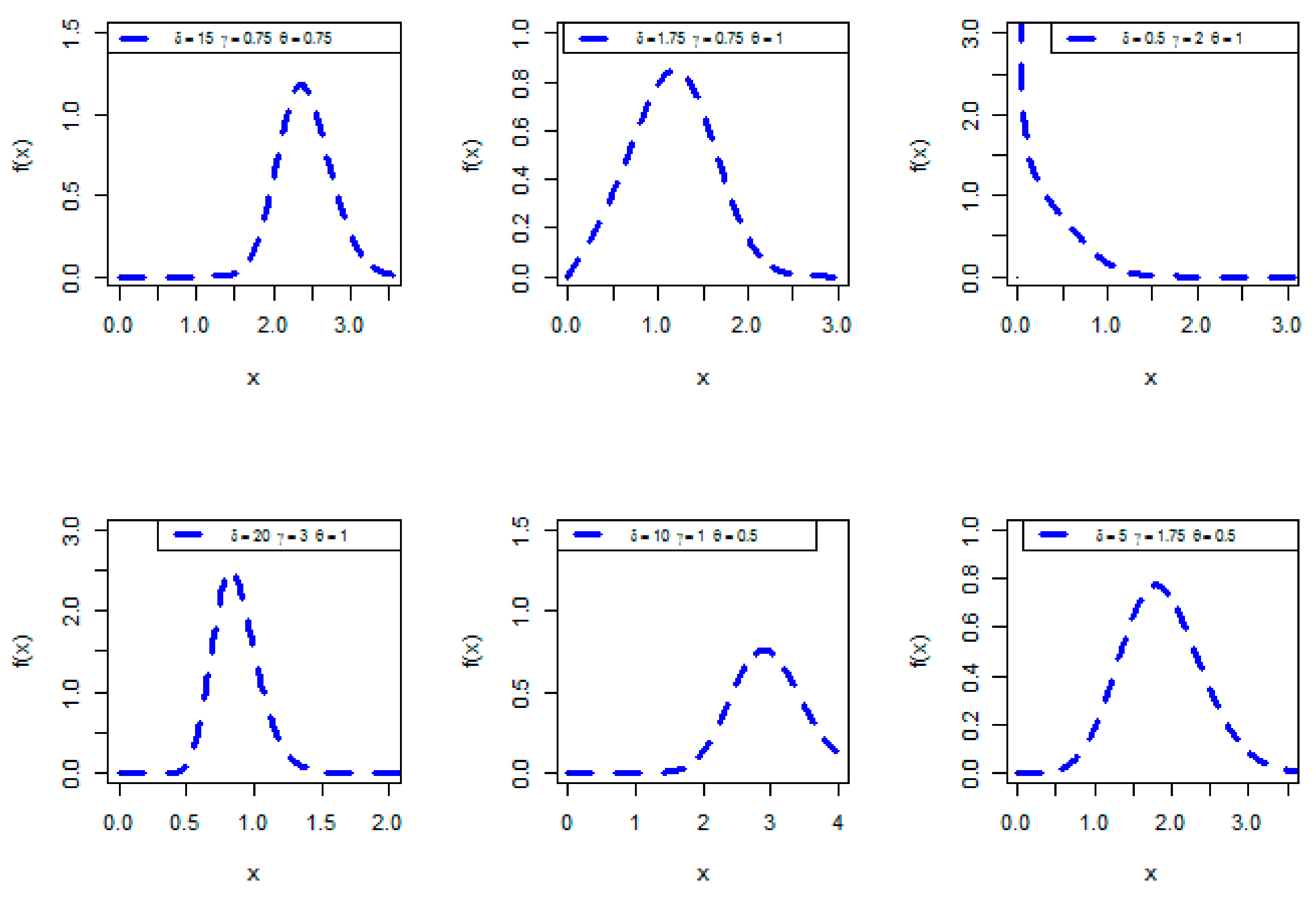
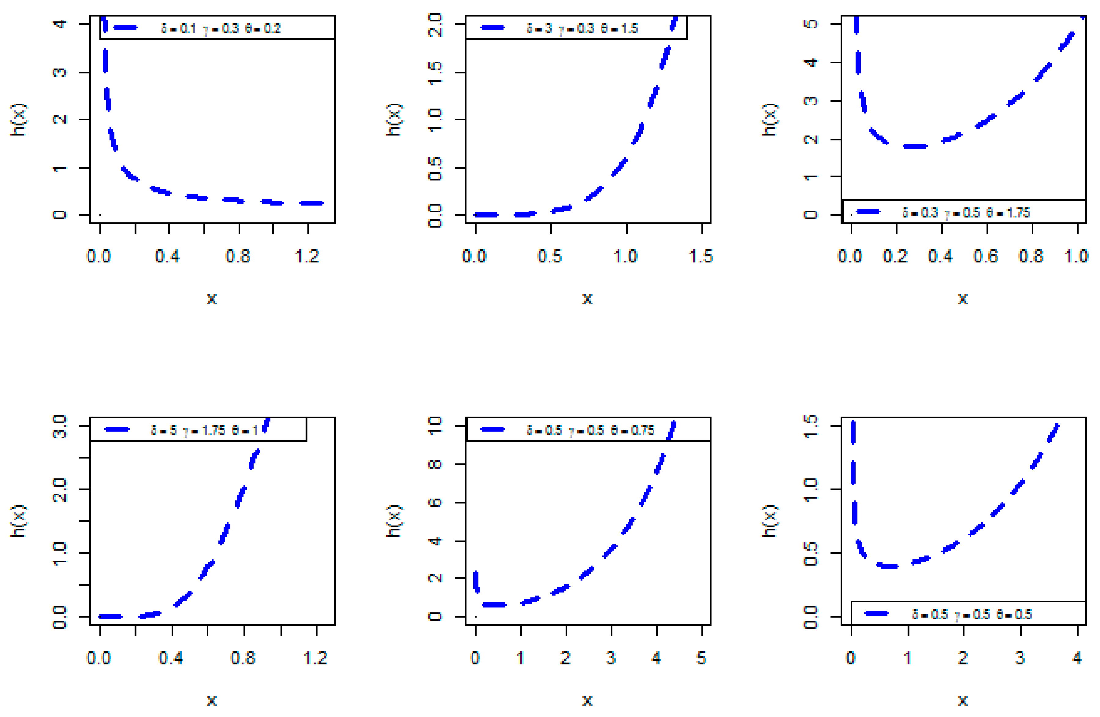
Afify et al. [14] studied many properties of the OEHLE distribution in explicit forms including quantile function, moments, moment generating function, mean inactivity time and mean residual life. They also provided some characterisations and showed its importance in practice by analysing two real data sets from the engineering field. They only used the maximum likelihood method to estimate the OEHLE parameters as the most popular estimation method. Some shapes of the density and hazard functions are depicted in Figure 1 and Figure 2.

Due to the significant role of parameter estimation in practice, our objective in this paper is to estimate the OEHLE parameters using frequentist estimation approaches namely, the maximum likelihood, maximum product spacing, least squares, Cramér–von-Mises, weighted least squares, Anderson–Darling, percentiles, and right-tail Anderson–Darling. Parameter estimation can also provide a guideline for choosing the best method of estimation for the OEHLE model, which would be very important to reliability engineers and applied statisticians (see Section 3). Furthermore, we compared these estimation methods using an extensive simulation study to address their performance. Finally, we showed that the OEHLE distribution can provide better fits than other competing exponential distributions using a real-life data set from engineering science.

Recently, statisticians have been very interested in comparing different classical estimation methods for estimating the parameters of several distributions. For example, the generalised Rayleigh (Kundu and Raqab [16]), weighted Lindley (Mazucheli et al. [17]), exponentiated-Chen (Dey et al. [18]), alpha logarithmic transformed Weibull (Nassar et al. [19]), transmuted exponentiated Pareto (Nassar et al. [20]), half-logistic Lomax (Aldahlan [21]), quasi xgamma-geometric (Sen et al. [22]), Weibull Marshall–Olkin Lindley (Afify et al. [23]), logarithmic transformed Weibull (Nassar et al. [24]).

This paper can be outlined as follows. In Section 2, different frequentist estimators are derived for the OEHLE parameters. We conduct a detailed simulation study to compare the different estimation approaches in Section 3. In Section 4, we discuss the potentiality of the OEHLE distribution by analysing real data from the engineering field. We provide some final remarks in Section 5.

2. Estimation Methods

This Section discusses the estimation of the OEHLE parameters, $\delta ,\gamma$ and $\theta$, via eight classical estimation approaches. These approaches are called the maximum likelihood, maximum product of spacing, least squares, Cramér–von-Mises, weighted least squares, percentiles, Anderson–Darling, and right-tail Anderson–Darling methods.

2.1. Maximum Likelihood Estimators

This subsection discusses the maximum likelihood estimators (MLEs) of the OEHLE parameters $\delta ,\gamma$ and $\theta .$

Let $X_1,X_2,\dots ,X_n$ be a random sample from the OEHLE with PDF (4). Then, for $\mathit{\varphi }={(\delta ,\gamma ,\theta )}^{⊺}$, the log-likelihood function $\ell \left(\mathit{\varphi };\mathit{x}\right)=\ell$ is:

$$\begin{array}{c}\ell =n\log \left(2 \gamma \delta \theta \right)+\theta {\displaystyle {\displaystyle \sum }_{i=1}^n}{x}_i+\gamma {\displaystyle {\displaystyle \sum }_{i=1}^n}\left(1-e^{\theta x_i}\right)\hfill \\ \hfill +\left(\delta -1\right){\displaystyle {\displaystyle \sum }_{i=1}^n}\log \left(1-{\mathrm{e}}^{\gamma \left(1-e^{\theta x_i}\right)}\right)-\left(\delta +1\right){\displaystyle {\displaystyle \sum }_{i=1}^n}\log \left(1+{\mathrm{e}}^{\gamma \left(1-e^{\theta x_i}\right)}\right).\end{array}$$

The MLEs for the parameters $\delta ,\gamma$ and $\theta$ can be obtaind by maximizing the log-likelihood function or by solving the following differential equations with respect to $\delta ,\gamma$ and $\theta$:

$$\frac{\partial \ell }{\partial \delta }=\frac{n}{\delta }+{\displaystyle \sum }_{i=1}^n\log \left(1-{\mathrm{e}}^{\gamma \left(1-e^{\theta x_i}\right)}\right)-{\displaystyle \sum }_{i=1}^n\log \left(1+{\mathrm{e}}^{\gamma \left(1-e^{\theta x_i}\right)}\right)=0,$$

(5)

$$\frac{\partial \ell }{\partial \gamma }=\frac{n}{\gamma }+{\displaystyle \sum }_{i=1}^n\left[1-e^{\theta x_i}\right]-\left(\delta -1\right){\displaystyle \sum }_{i=1}^n\frac{\left(1-e^{\theta x_i}\right){\mathrm{e}}^{\gamma \left(1-e^{\theta x_i}\right)}}{1-{\mathrm{e}}^{\gamma \left(1-e^{\theta x_i}\right)}}-\left(\delta +1\right){\displaystyle \sum }_{i=1}^n\frac{\left[1-\exp \left(\theta x_i\right)\right]{\mathrm{e}}^{\gamma \left(1-e^{\theta x_i}\right)}}{1+{\mathrm{e}}^{\gamma \left(1-e^{\theta x_i}\right)}}=0$$

(6)

and:

$$\begin{gathered} \frac{\partial \ell }{\partial \theta }=\frac{n}{\theta }-{\displaystyle \sum }_{i=1}^n{x}_i-\gamma {\displaystyle \sum }_{i=1}^n\frac{x_i{e}^{\theta x_i}}{1-e^{\theta x_i}}+\left(\delta -1\right){\displaystyle \sum }_{i=1}^n\frac{\mathsf{\gamma }{x}_i{e}^{\theta x_i}{\mathrm{e}}^{\gamma \left(1-e^{\theta x_i}\right)}}{1-{\mathrm{e}}^{\gamma \left(1-e^{\theta x_i}\right)}} \\ +\left(\delta +1\right){\displaystyle \sum }_{i=1}^n\frac{\mathsf{\gamma }{x}_i{e}^{\theta x_i}{\mathrm{e}}^{\gamma \left(1-e^{\theta x_i}\right)}}{1+{\mathrm{e}}^{\gamma \left(1-e^{\theta x_i}\right)}}=0. \end{gathered}$$

(7)

Equations (5)–(7) can be maximized using various programs such as Mathematica, Mathcad, SAS (PROC NLMIXED) and $R$ (optim function).

2.2. Maximum Product of Spacing Estimators

The maximum product of spacing estimators (MPSEs) due to Cheng and Amin [25,26] and Ranneby [27]. Ranneby [27] proved, in some situations, that the maximum product of spacing (MPS) estimate asymptotically has the same properties as the maximum likelihood (ML) estimate and that the MSP method gives consistent estimates, but the ML method does not, hence, the MPSEs can be considered a good alternative to the MLEs. Consider the order statistics of a random sample from the OEHLE distribution, denoted by $x_{\left(1:n\right)},x_{\left(2:n\right)},\cdots ,x_{\left(n:n\right)},$ and consider the uniform spacings for this random sample:

$$D_i\left(\delta ,\gamma ,\theta \right)=F\left(x_{\left(i\right)}|\delta ,\gamma ,\theta \right)-F\left(x_{\left(i-1\right)}|\delta ,\gamma ,\theta \right), \mathrm{for} i=1,2,\dots ,n+1,$$

where $F\left(x_{\left(0\right)}|\delta ,\gamma ,\theta \right)=0$, $F\left(x_{\left(n+1\right)}|\delta ,\gamma ,\theta \right)=1,{{\displaystyle \sum }}_{i=1}^{n+1}{D}_i\left(\delta ,\gamma ,\theta \right)=1,$

$$F\left(x_{\left(i\right)}|\delta ,\gamma ,\theta \right)={\left[\frac{1-{\mathrm{e}}^{\gamma \left(1-e^{\theta x_{\left(i\right)}}\right)}}{1+{\mathrm{e}}^{\gamma \left(1-e^{\theta x_{\left(i\right)}}\right)}}\right]}^{\delta }\mathrm{and} F\left(x_{\left(i-1\right)}|\delta ,\gamma ,\theta \right)={\left[\frac{1-{\mathrm{e}}^{\gamma \left(1-e^{\theta x_{\left(i-1\right)}}\right)}}{1+{\mathrm{e}}^{\gamma \left(1-e^{\theta x_{\left(i-1\right)}}\right)}}\right]}^{\delta }.$$

Then, the MPSEs of ${\widehat{\delta }}_{MPSE},$ ${\widehat{\gamma }}_{MPSE}$ and ${\widehat{\theta }}_{MPSE}$ follow by maximizing either the geometric mean of spacings or the logarithm of the sample geometric mean spacings which are defined by

$$\mathrm{MS}\left(\delta ,\gamma ,\theta \right)={\left[{\displaystyle \prod }_{i=1}^{n+1} D_i\left(\gamma ,\delta ,\theta \right)\right]}^{\frac{1}{n+1}}$$

and:

$$LM\left(\delta ,\gamma ,\theta \right)=\frac{1}{n+1}{\displaystyle \sum }_{i=1}^{n+1}\log \left[D_i\left(\delta ,\gamma ,\theta \right)\right],$$

with respect to $\delta ,\gamma$ and $\theta$.

The MPSEs of the OEHLE parameters can also be obtained by solving the following nonlinear equations:

$$\frac{1}{n+1}{\displaystyle \sum }_{i=1}^{n+1}\frac{1}{D_i\left(\delta ,\gamma ,\theta \right)}\left[{\Delta }_r(x_{\left(i\right)}|\delta ,\gamma ,\theta )-{\Delta }_r(x_{\left(i-1\right)}|\delta ,\gamma ,\theta )\right]=0, \mathrm{for} r=1,2,3,$$

where:

$$\begin{gathered} {\Delta }_1\left(x_{\left(i\right)}|\delta ,\gamma ,\theta \right)=\frac{\partial }{\partial \delta }F\left(x_{\left(i\right)}|\delta ,\gamma ,\theta \right), {\Delta }_2\left(x_{\left(i\right)}|\delta ,\gamma ,\theta \right)=\frac{\partial }{\partial \gamma }F\left(x_{\left(i\right)}|\delta ,\gamma ,\theta \right) \mathrm{and} \\ {\Delta }_3\left(x_{\left(i\right)}|\delta ,\gamma ,\theta \right)=\frac{\partial }{\partial \theta }F\left(x_{\left(i\right)}|\delta ,\gamma ,\theta \right). \end{gathered}$$

(8)

It is worth mentioning that ${\Delta }_r$ for $r=1,2,3$ can be solved numerically.

2.3. Least Squares and Weighted Least Squares Estimators

Consider the order statistics of a random sample from the OEHLE distribution denoted by $x_{\left(1:n\right)},x_{\left(2:n\right)},\cdots ,x_{\left(n:n\right)}.$ The least squares estimators (LSEs) (Swain et al. [28]) of the OEHLE parameters ${\widehat{\delta }}_{LSE}$, ${\widehat{\gamma }}_{LSE}$ and ${\widehat{\theta }}_{LSE}$ follow by minimizing:

$$L\left(\delta ,\gamma ,\theta \right)={\displaystyle \sum }_{i=1}^n{\left[F\left(x_{\left(i:n\right)}|\delta ,\gamma ,\theta \right)-\left(\frac{i}{n+1}\right)\right]}^2,$$

with respect to $\delta , \gamma$ and $\theta$. Or equivalently, the LSEs are obtained by solving the non-linear equations:

$${\displaystyle \sum }_{i=1}^n\left[F\left(x_{\left(i:n\right)}|\delta ,\gamma ,\theta \right)-\left(\frac{i}{n+1}\right)\right]{\Delta }_r\left(x_{\left(i:n\right)}|\delta ,\gamma ,\theta \right)=0, r=1,2,3,$$

where ${\Delta }_1\left(·|\delta ,\gamma ,\theta \right)$, ${\Delta }_2\left(·|\delta ,\gamma ,\theta \right)$ and ${\Delta }_3\left(·|\delta ,\gamma ,\theta \right)$ are given in (8).

The weighted least-squares estimators (WLSEs) of the OEHLE parameters ${\widehat{\delta }}_{WLSE},{\widehat{\gamma }}_{WLSE}$ and ${\widehat{\theta }}_{WLSE}$, can be derived by minimizing the following equation with respect to the parameters:

$$W\left(\delta ,\gamma ,\theta \right)={\displaystyle \sum }_{i=1}^n\frac{{\left(n+1\right)}^2\left(n+2\right)}{i\left(n-i+1\right)}{\left[F\left(x_{\left(i:n\right)}|\delta ,\gamma ,\theta \right)-\frac{i}{n+1}\right]}^2.$$

Furthermore, the WLSEs can also be calculated by solving the following non-linear equations:

$${\displaystyle \sum }_{i=1}^n\frac{{\left(n+1\right)}^2\left(n+2\right)}{i\left(n-i+1\right)}\left[F\left(x_{\left(i:n\right)}|\delta ,\gamma ,\theta \right)-\frac{i}{n+1}\right]{\Delta }_r\left(x_{\left(i:n\right)}|\delta ,\gamma ,\theta \right)=0, r=1,2,3$$

where ${\Delta }_1\left(·|\delta ,\gamma ,\theta \right)$, ${\Delta }_2\left(·|\delta ,\gamma ,\theta \right)$ and ${\Delta }_3\left(·|\delta ,\gamma ,\theta \right)$ are given in (8).

2.4. Cramér–von Mises Estimators

The Cramér–von Mises estimators (CVMEs) due to Macdonald [29] are a type of minimum distance estimator and have less bias than other minimum distance estimators. The CVMEs can be derived as the difference between the estimates of the CDF and the empirical CDF (Luceno [30]). The CVMEs of the OEHLE parameters can be obtained by minimizing the following equation with respect to $\delta ,\gamma$ and $\theta$:

$$C\left(\delta ,\gamma ,\theta \right)=\frac{1}{12n}+{\displaystyle \sum }_{i=1}^n{\left[F\left(x_{\left(i:n\right)}|\delta ,\gamma ,\theta \right)-\left(\frac{2i-1}{2n}\right)\right]}^2,$$

The CVMEs can also follow by solving the following non-linear equations:

$${\displaystyle \sum }_{i=1}^n\left[F\left(x_{\left(i:n\right)}|\delta ,\gamma ,\theta \right)-\left(\frac{2i-1}{2n}\right)\right]{\Delta }_r\left(x_{\left(i:n\right)}|\delta ,\gamma ,\theta \right)=0, r=1,2,3,$$

where ${\Delta }_1\left(·|\delta ,\gamma ,\theta \right)$, ${\Delta }_2\left(·|\delta ,\gamma ,\theta \right)$ and ${\Delta }_3\left(·|\delta ,\gamma ,\theta \right)$ are given in (8).

2.5. Percentiles Estimators

The percentiles approach is proposed by Kao [31,32]. Consider an unbiased estimator of $F\left(x_{\left(i:n\right)}|\delta ,\gamma ,\theta \right)$ given by $u_i=i/\left(1+n\right)$. Then, the percentile estimators (PCEs) of the OEHLE parameters can be derived by minimizing this function:

$$P\left(\gamma ,\delta ,\theta \right)={\displaystyle \sum }_{i=1}^n{\left\{x_{\left(i:n\right)}+\frac{1}{\theta }\log \left[1-\frac{\log \left(1+q_i^{\frac{1}{\delta }}\right)-\log \left(1-q_i^{\frac{1}{\delta }}\right)}{\gamma +\log \left(1+q_i^{\frac{1}{\delta }}\right)-\log \left(1-q_i^{\frac{1}{\delta }}\right)}\right]\right\}}^2,$$

with respect to $\delta ,\gamma$ and $\theta$, where $q_i=i/\left(1+n\right)$ is an estimate of $F\left(x_{\left(i:n\right)}|\delta ,\gamma ,\theta \right)$.

2.6. The Anderson–Darling and Right-Tail Anderson–Darling Estimators

The Anderson–Darling estimators (ANDEs) are considered a type of minimum distance estimators. The ANDEs of the OEHLE parameters can be derived by minimizing:

$$A\left(\delta ,\gamma ,\theta \right)=-n-\frac{1}{n}{\displaystyle \sum }_{i=1}^n\left(2i-1\right) \left\{\log \left[F\left(x_{\left(i:n\right)}|\delta ,\gamma ,\theta \right)\right]+\log \left[\overline{F}\left(x_{\left(i:n\right)}|\delta ,\gamma ,\theta \right)\right]\right\},$$

with respect to $\delta ,\gamma$ and $\theta$. These estimators are also derived by solving the following non-linear equations:

$${\displaystyle \sum }_{i=1}^n\left(2i-1\right)\left[\frac{{\Delta }_r\left(x_{\left(i:n\right)}|\delta ,\gamma ,\theta \right)}{F\left(x_{\left(i:n\right)}|\delta ,\gamma ,\theta \right)}-\frac{{\Delta }_j\left(x_{\left(n+1-i:n\right)}|\delta ,\gamma ,\theta \right)}{\overline{F}\left(x_{\left(n+1-i:n\right)}|\delta ,\gamma ,\theta \right)}\right]=0, r,j=1,2,3,$$

where ${\Delta }_1\left(·|\delta ,\gamma ,\theta \right)$, ${\Delta }_2\left(·|\delta ,\gamma ,\theta \right)$ and ${\Delta }_3\left(·|\delta ,\gamma ,\theta \right)$ are given in (8) and:

$$\overline{F}\left(x_{\left(n+1-i:n\right)}|\delta ,\gamma ,\theta \right)=1-{\left[\frac{1-{\mathrm{e}}^{\gamma \left(1-e^{\theta x_{\left(n+1-i\right)}}\right)}}{1+{\mathrm{e}}^{\gamma \left(1-e^{\theta x_{\left(n+1-i\right)}}\right)}}\right]}^{\delta }.$$

The right-tail Anderson–Darling estimators (RANDEs) of the OEHLE parameters can be derived by minimizing:

$$R\left(\delta ,\gamma ,\theta \right)=\frac{n}{2}-2{\displaystyle \sum }_{i=1}^{n}F\left(x_{\left(i:n\right)}|\delta ,\gamma ,\theta \right)-\frac{1}{n}{\displaystyle \sum }_{i=1}^n\left(2i-1\right)\log \left[\overline{F}\left(x_{\left(n+1-i:n\right)}|\delta ,\gamma ,\theta \right)\right],$$

with respect to $\delta ,\gamma$ and $\theta$. The RANDEs are also derived by solving the following non-linear equations:

$$-2{\displaystyle \sum }_{i=1}^n{\Delta }_r\left(x_{\left(i:n\right)}|\delta ,\gamma ,\theta \right)+\frac{1}{n}{\displaystyle \sum }_{i=1}^n\left(2i-1\right)\frac{{\Delta }_r\left(x_{{ }_{\left(n+1-i:n\right)}}|\delta ,\gamma ,\theta \right)}{\overline{F}\left(x_{\left(n+1-i:n\right)}|\delta ,\gamma ,\theta \right)}=0, r=1,2,3,$$

where ${\Delta }_1\left(·|\delta ,\gamma ,\theta \right)$, ${\Delta }_2\left(·|\delta ,\gamma ,\theta \right)$ and ${\Delta }_3\left(·|\delta ,\gamma ,\theta \right)$ are given in (5).

3. Simulation Results

We performed a detailed simulation study to compare and assess the performance of the considered eight different estimators of the OEHLE parameters. Using the R software (version 3.6.3), we generated 5000 samples from the OEHLE distribution for sample sizes, $n=20, 50, 100, 200, 400$ and for $\delta =0.75, 2.75$, $\gamma =0.5, 2.0$ and $\theta =0.67, 1.5$. For each sample and each parameter combination, we calculate the following measures: the average estimates (AVEs), mean square errors (MSEs) of the estimates, average absolute biases (AVBs), and mean relative errors (MREs) of the estimates.

In order to provide a guideline for choosing the best method of estimation for the OEHLE parameters, which would be very important to reliability engineers and applied statisticians, we calculated the partial and overall ranks of all methods of estimation for different parameter combinations.

Table A1. Simulation results of several estimation methods for $\delta =0.75,$ $\gamma =0.50$ and $\theta =0.67$.

$\mathit{n}$	Measures	Pa.	MLEs	MPSEs	LSEs	CVMEs	WLSEs	PCEs	ANDEs	RANDEs
20	AVEs	$\delta$	${0.75733}^{\left\{5\right\}}$	${0.61377}^{\left\{1\right\}}$	${0.66358}^{\left\{2\right\}}$	${0.77453}^{\left\{7\right\}}$	${0.68297}^{\left\{3\right\}}$	${0.76283}^{\left\{6\right\}}$	${0.73015}^{\left\{4\right\}}$	${0.92063}^{\left\{8\right\}}$
		$\gamma$	${0.34798}^{\left\{1\right\}}$	${0.45428}^{\left\{2\right\}}$	${0.49052}^{\left\{5\right\}}$	${0.53795}^{\left\{7\right\}}$	${0.48938}^{\left\{4\right\}}$	${0.49843}^{\left\{6\right\}}$	${0.47743}^{\left\{3\right\}}$	${0.55800}^{\left\{8\right\}}$
		$\theta$	${0.68080}^{\left\{4\right\}}$	${0.73651}^{\left\{7\right\}}$	${0.74151}^{\left\{8\right\}}$	${0.71479}^{\left\{6\right\}}$	${0.66463}^{\left\{2\right\}}$	${0.66787}^{\left\{3\right\}}$	${0.68126}^{\left\{5\right\}}$	${0.61779}^{\left\{1\right\}}$
	MSEs	$\delta$	${0.04872}^{\left\{1\right\}}$	${0.30451}^{\left\{4\right\}}$	${0.35538}^{\left\{6\right\}}$	${0.38795}^{\left\{8\right\}}$	${0.06060}^{\left\{3\right\}}$	${0.31609}^{\left\{5\right\}}$	${0.05151}^{\left\{2\right\}}$	${0.38176}^{\left\{7\right\}}$
		$\gamma$	${0.18475}^{\left\{7\right\}}$	${0.02825}^{\left\{1\right\}}$	${0.03258}^{\left\{3\right\}}$	${0.03404}^{\left\{4\right\}}$	${0.20933}^{\left\{8\right\}}$	${0.03201}^{\left\{2\right\}}$	${0.17981}^{\left\{6\right\}}$	${0.03706}^{\left\{5\right\}}$
		$\theta$	${0.11825}^{\left\{7\right\}}$	${0.10703}^{\left\{6\right\}}$	${0.10580}^{\left\{4\right\}}$	${0.10693}^{\left\{5\right\}}$	${0.14271}^{\left\{8\right\}}$	${0.09750}^{\left\{2\right\}}$	${0.10125}^{\left\{3\right\}}$	${0.09713}^{\left\{1\right\}}$
	AVBs	$\delta$	${0.22073}^{\left\{1\right\}}$	${0.55183}^{\left\{4\right\}}$	${0.59613}^{\left\{6\right\}}$	${0.62286}^{\left\{8\right\}}$	${0.24617}^{\left\{3\right\}}$	${0.56222}^{\left\{5\right\}}$	${0.22696}^{\left\{2\right\}}$	${0.61786}^{\left\{7\right\}}$
		$\gamma$	${0.42982}^{\left\{7\right\}}$	${0.16806}^{\left\{1\right\}}$	${0.18050}^{\left\{3\right\}}$	${0.18450}^{\left\{4\right\}}$	${0.45753}^{\left\{8\right\}}$	${0.17891}^{\left\{2\right\}}$	${0.42404}^{\left\{6\right\}}$	${0.19251}^{\left\{5\right\}}$
		$\theta$	${0.34387}^{\left\{7\right\}}$	${0.32716}^{\left\{6\right\}}$	${0.32526}^{\left\{4\right\}}$	${0.32700}^{\left\{5\right\}}$	${0.37777}^{\left\{8\right\}}$	${0.31225}^{\left\{2\right\}}$	${0.31819}^{\left\{3\right\}}$	${0.31166}^{\left\{1\right\}}$
	MREs	$\delta$	${0.29430}^{\left\{1\right\}}$	${0.73577}^{\left\{4\right\}}$	${0.79485}^{\left\{6\right\}}$	${0.83048}^{\left\{8\right\}}$	${0.32823}^{\left\{3\right\}}$	${0.74962}^{\left\{5\right\}}$	${0.30261}^{\left\{2\right\}}$	${0.82382}^{\left\{7\right\}}$
		$\gamma$	${0.85965}^{\left\{7\right\}}$	${0.33613}^{\left\{1\right\}}$	${0.36100}^{\left\{3\right\}}$	${0.36899}^{\left\{4\right\}}$	${0.91506}^{\left\{8\right\}}$	${0.35781}^{\left\{2\right\}}$	${0.84807}^{\left\{6\right\}}$	${0.38501}^{\left\{5\right\}}$
		$\theta$	${0.51324}^{\left\{7\right\}}$	${0.48830}^{\left\{6\right\}}$	${0.48546}^{\left\{4\right\}}$	${0.48805}^{\left\{5\right\}}$	${0.56384}^{\left\{8\right\}}$	${0.46604}^{\left\{2\right\}}$	${0.47492}^{\left\{3\right\}}$	${0.46516}^{\left\{1\right\}}$
	$\mathbf{\sum }\mathit{R}\mathit{a}\mathit{n}\mathit{k}\mathit{s}$		${\mathbf{55}}^{\left\{\mathbf{5}\right\}}$	${\mathbf{43}}^{\left\{\mathbf{2}\right\}}$	${\mathbf{54}}^{\left\{\mathbf{4}\right\}}$	${\mathbf{71}}^{\left\{\mathbf{8}\right\}}$	${\mathbf{66}}^{\left\{\mathbf{7}\right\}}$	${\mathbf{42}}^{\left\{\mathbf{1}\right\}}$	${\mathbf{45}}^{\left\{\mathbf{3}\right\}}$	${\mathbf{56}}^{\left\{\mathbf{6}\right\}}$
50	AVEs	$\delta$	${0.75829}^{\left\{5\right\}}$	${0.71838}^{\left\{1\right\}}$	${0.72642}^{\left\{3\right\}}$	${0.76235}^{\left\{6\right\}}$	${0.72358}^{\left\{2\right\}}$	${0.84359}^{\left\{8\right\}}$	${0.74484}^{\left\{4\right\}}$	${0.82110}^{\left\{7\right\}}$
		$\gamma$	${0.42639}^{\left\{1\right\}}$	${0.48486}^{\left\{3\right\}}$	${0.49714}^{\left\{5\right\}}$	${0.51011}^{\left\{6\right\}}$	${0.46889}^{\left\{2\right\}}$	${0.52468}^{\left\{8\right\}}$	${0.49153}^{\left\{4\right\}}$	${0.52029}^{\left\{7\right\}}$
		$\theta$	${0.66030}^{\left\{3\right\}}$	${0.66795}^{\left\{4\right\}}$	${0.68974}^{\left\{8\right\}}$	${0.68129}^{\left\{7\right\}}$	${0.67681}^{\left\{6\right\}}$	${0.61784}^{\left\{1\right\}}$	${0.67660}^{\left\{5\right\}}$	${0.64881}^{\left\{2\right\}}$
	MSEs	$\delta$	${0.02145}^{\left\{2\right\}}$	${0.15997}^{\left\{4\right\}}$	${0.28138}^{\left\{7\right\}}$	${0.29906}^{\left\{8\right\}}$	${0.02225}^{\left\{3\right\}}$	${0.23453}^{\left\{5\right\}}$	${0.01870}^{\left\{1\right\}}$	${0.25563}^{\left\{6\right\}}$
		$\gamma$	${0.09885}^{\left\{7\right\}}$	${0.01667}^{\left\{1\right\}}$	${0.02386}^{\left\{3\right\}}$	${0.02318}^{\left\{2\right\}}$	${0.10569}^{\left\{8\right\}}$	${0.02439}^{\left\{4\right\}}$	${0.09181}^{\left\{6\right\}}$	${0.02440}^{\left\{5\right\}}$
		$\theta$	${0.04187}^{\left\{2\right\}}$	${0.08705}^{\left\{4\right\}}$	${0.09635}^{\left\{7\right\}}$	${0.09740}^{\left\{8\right\}}$	${0.04472}^{\left\{3\right\}}$	${0.09303}^{\left\{5\right\}}$	${0.03648}^{\left\{1\right\}}$	${0.09345}^{\left\{6\right\}}$
	AVBs	$\delta$	${0.14647}^{\left\{2\right\}}$	${0.39997}^{\left\{4\right\}}$	${0.53045}^{\left\{7\right\}}$	${0.54687}^{\left\{8\right\}}$	${0.14916}^{\left\{3\right\}}$	${0.48428}^{\left\{5\right\}}$	${0.13674}^{\left\{1\right\}}$	${0.50560}^{\left\{6\right\}}$
		$\gamma$	${0.31440}^{\left\{7\right\}}$	${0.12911}^{\left\{1\right\}}$	${0.15447}^{\left\{3\right\}}$	${0.15224}^{\left\{2\right\}}$	${0.32510}^{\left\{8\right\}}$	${0.15617}^{\left\{4\right\}}$	${0.30300}^{\left\{6\right\}}$	${0.15620}^{\left\{5\right\}}$
		$\theta$	${0.20463}^{\left\{2\right\}}$	${0.29505}^{\left\{4\right\}}$	${0.31041}^{\left\{7\right\}}$	${0.31209}^{\left\{8\right\}}$	${0.21146}^{\left\{3\right\}}$	${0.30501}^{\left\{5\right\}}$	${0.19100}^{\left\{1\right\}}$	${0.30570}^{\left\{6\right\}}$
	MREs	$\delta$	${0.19529}^{\left\{2\right\}}$	${0.53329}^{\left\{4\right\}}$	${0.70727}^{\left\{7\right\}}$	${0.72915}^{\left\{8\right\}}$	${0.19888}^{\left\{3\right\}}$	${0.64571}^{\left\{5\right\}}$	${0.18232}^{\left\{1\right\}}$	${0.67413}^{\left\{6\right\}}$
		$\gamma$	${0.62880}^{\left\{7\right\}}$	${0.25823}^{\left\{1\right\}}$	${0.30893}^{\left\{3\right\}}$	${0.30449}^{\left\{2\right\}}$	${0.65019}^{\left\{8\right\}}$	${0.31234}^{\left\{4\right\}}$	${0.60599}^{\left\{6\right\}}$	${0.31241}^{\left\{5\right\}}$
		$\theta$	${0.30542}^{\left\{2\right\}}$	${0.44037}^{\left\{4\right\}}$	${0.46330}^{\left\{7\right\}}$	${0.46581}^{\left\{8\right\}}$	${0.31562}^{\left\{3\right\}}$	${0.45524}^{\left\{5\right\}}$	${0.28507}^{\left\{1\right\}}$	${0.45626}^{\left\{6\right\}}$
	$\mathbf{\sum }\mathit{R}\mathit{a}\mathit{n}\mathit{k}\mathit{s}$		${\mathbf{42}}^{\left\{\mathbf{3}\right\}}$	${\mathbf{35}}^{\left\{\mathbf{1}\right\}}$	${\mathbf{67}}^{\left\{\mathbf{6.5}\right\}}$	${\mathbf{73}}^{\left\{\mathbf{8}\right\}}$	${\mathbf{52}}^{\left\{\mathbf{4}\right\}}$	${\mathbf{59}}^{\left\{\mathbf{5}\right\}}$	${\mathbf{37}}^{\left\{\mathbf{2}\right\}}$	${\mathbf{67}}^{\left\{\mathbf{6.5}\right\}}$
100	AVEs	$\delta$	${0.75589}^{\left\{5\right\}}$	${0.73810}^{\left\{2\right\}}$	${0.72147}^{\left\{1\right\}}$	${0.75688}^{\left\{6\right\}}$	${0.74086}^{\left\{3\right\}}$	${0.85749}^{\left\{8\right\}}$	${0.74597}^{\left\{4\right\}}$	${0.80590}^{\left\{7\right\}}$
		$\gamma$	${0.45205}^{\left\{1\right\}}$	${0.49441}^{\left\{2\right\}}$	${0.49507}^{\left\{3\right\}}$	${0.50594}^{\left\{6\right\}}$	${0.49641}^{\left\{5\right\}}$	${0.53126}^{\left\{8\right\}}$	${0.49606}^{\left\{4\right\}}$	${0.51752}^{\left\{7\right\}}$
		$\theta$	${0.65441}^{\left\{3\right\}}$	${0.65651}^{\left\{4\right\}}$	${0.68936}^{\left\{8\right\}}$	${0.67801}^{\left\{7\right\}}$	${0.66731}^{\left\{5\right\}}$	${0.60603}^{\left\{1\right\}}$	${0.67379}^{\left\{6\right\}}$	${0.64518}^{\left\{2\right\}}$
	MSEs	$\delta$	${0.01064}^{\left\{3\right\}}$	${0.08325}^{\left\{4\right\}}$	${0.16963}^{\left\{7\right\}}$	${0.17824}^{\left\{8\right\}}$	${0.01024}^{\left\{2\right\}}$	${0.15920}^{\left\{6\right\}}$	${0.00977}^{\left\{1\right\}}$	${0.15096}^{\left\{5\right\}}$
		$\gamma$	${0.05057}^{\left\{7\right\}}$	${0.00892}^{\left\{1\right\}}$	${0.01466}^{\left\{3\right\}}$	${0.01501}^{\left\{4\right\}}$	${0.05261}^{\left\{8\right\}}$	${0.01543}^{\left\{5\right\}}$	${0.05020}^{\left\{6\right\}}$	${0.01436}^{\left\{2\right\}}$
		$\theta$	${0.01801}^{\left\{2\right\}}$	${0.04424}^{\left\{4\right\}}$	${0.09110}^{\left\{7\right\}}$	${0.09199}^{\left\{8\right\}}$	${0.01948}^{\left\{3\right\}}$	${0.08734}^{\left\{5\right\}}$	${0.01793}^{\left\{1\right\}}$	${0.08811}^{\left\{6\right\}}$
	AVBs	$\delta$	${0.10313}^{\left\{3\right\}}$	${0.28853}^{\left\{4\right\}}$	${0.41186}^{\left\{7\right\}}$	${0.42219}^{\left\{8\right\}}$	${0.10118}^{\left\{2\right\}}$	${0.39900}^{\left\{6\right\}}$	${0.09885}^{\left\{1\right\}}$	${0.38854}^{\left\{5\right\}}$
		$\gamma$	${0.22488}^{\left\{7\right\}}$	${0.09442}^{\left\{1\right\}}$	${0.12109}^{\left\{3\right\}}$	${0.12251}^{\left\{4\right\}}$	${0.22937}^{\left\{8\right\}}$	${0.12423}^{\left\{5\right\}}$	${0.22406}^{\left\{6\right\}}$	${0.11984}^{\left\{2\right\}}$
		$\theta$	${0.13419}^{\left\{2\right\}}$	${0.21033}^{\left\{4\right\}}$	${0.30182}^{\left\{7\right\}}$	${0.30330}^{\left\{8\right\}}$	${0.13958}^{\left\{3\right\}}$	${0.29553}^{\left\{5\right\}}$	${0.13391}^{\left\{1\right\}}$	${0.29683}^{\left\{6\right\}}$
	MREs	$\delta$	${0.13751}^{\left\{3\right\}}$	${0.38471}^{\left\{4\right\}}$	${0.54915}^{\left\{7\right\}}$	${0.56292}^{\left\{8\right\}}$	${0.13491}^{\left\{2\right\}}$	${0.53201}^{\left\{6\right\}}$	${0.13180}^{\left\{1\right\}}$	${0.51805}^{\left\{5\right\}}$
		$\gamma$	${0.44976}^{\left\{7\right\}}$	${0.18884}^{\left\{1\right\}}$	${0.24218}^{\left\{3\right\}}$	${0.24501}^{\left\{4\right\}}$	${0.45874}^{\left\{8\right\}}$	${0.24845}^{\left\{5\right\}}$	${0.44812}^{\left\{6\right\}}$	${0.23969}^{\left\{2\right\}}$
		$\theta$	${0.20029}^{\left\{2\right\}}$	${0.31392}^{\left\{4\right\}}$	${0.45048}^{\left\{7\right\}}$	${0.45269}^{\left\{8\right\}}$	${0.20833}^{\left\{3\right\}}$	${0.44110}^{\left\{5\right\}}$	${0.19986}^{\left\{1\right\}}$	${0.44303}^{\left\{6\right\}}$
	$\mathbf{\sum }\mathit{R}\mathit{a}\mathit{n}\mathit{k}\mathit{s}$		${\mathbf{45}}^{\left\{\mathbf{3}\right\}}$	${\mathbf{35}}^{\left\{\mathbf{1}\right\}}$	${\mathbf{63}}^{\left\{\mathbf{6}\right\}}$	${\mathbf{79}}^{\left\{\mathbf{8}\right\}}$	${\mathbf{52}}^{\left\{\mathbf{4}\right\}}$	${\mathbf{65}}^{\left\{\mathbf{7}\right\}}$	${\mathbf{38}}^{\left\{\mathbf{2}\right\}}$	${\mathbf{55}}^{\left\{\mathbf{5}\right\}}$
200	AVEs	$\delta$	${0.75200}^{\left\{6\right\}}$	${0.74714}^{\left\{4\right\}}$	${0.72918}^{\left\{1\right\}}$	${0.74128}^{\left\{2\right\}}$	${0.74453}^{\left\{3\right\}}$	${0.82035}^{\left\{8\right\}}$	${0.74828}^{\left\{5\right\}}$	${0.77522}^{\left\{7\right\}}$
		$\gamma$	${0.46515}^{\left\{1\right\}}$	${0.49797}^{\left\{4\right\}}$	${0.49323}^{\left\{2\right\}}$	${0.49959}^{\left\{5\right\}}$	${0.49749}^{\left\{3\right\}}$	${0.51922}^{\left\{8\right\}}$	${0.50608}^{\left\{6\right\}}$	${0.50756}^{\left\{7\right\}}$
		$\theta$	${0.65997}^{\left\{3\right\}}$	${0.66015}^{\left\{4\right\}}$	${0.68532}^{\left\{8\right\}}$	${0.68096}^{\left\{7\right\}}$	${0.66993}^{\left\{6\right\}}$	${0.62771}^{\left\{1\right\}}$	${0.66756}^{\left\{5\right\}}$	${0.65927}^{\left\{2\right\}}$
	MSEs	$\delta$	${0.00521}^{\left\{3\right\}}$	${0.04534}^{\left\{4\right\}}$	${0.09936}^{\left\{8\right\}}$	${0.09855}^{\left\{7\right\}}$	${0.00498}^{\left\{2\right\}}$	${0.08277}^{\left\{5\right\}}$	${0.00462}^{\left\{1\right\}}$	${0.08431}^{\left\{6\right\}}$
		$\gamma$	${0.02714}^{\left\{7\right\}}$	${0.00460}^{\left\{1\right\}}$	${0.00870}^{\left\{5\right\}}$	${0.00849}^{\left\{4\right\}}$	${0.02861}^{\left\{8\right\}}$	${0.00824}^{\left\{2\right\}}$	${0.02698}^{\left\{6\right\}}$	${0.00830}^{\left\{3\right\}}$
		$\theta$	${0.00928}^{\left\{1\right\}}$	${0.02201}^{\left\{4\right\}}$	${0.06137}^{\left\{7\right\}}$	${0.06244}^{\left\{8\right\}}$	${0.00987}^{\left\{3\right\}}$	${0.04046}^{\left\{5\right\}}$	${0.00949}^{\left\{2\right\}}$	${0.04477}^{\left\{6\right\}}$
	AVBs	$\delta$	${0.07221}^{\left\{3\right\}}$	${0.21293}^{\left\{4\right\}}$	${0.31522}^{\left\{8\right\}}$	${0.31392}^{\left\{7\right\}}$	${0.07055}^{\left\{2\right\}}$	${0.28770}^{\left\{5\right\}}$	${0.06795}^{\left\{1\right\}}$	${0.29036}^{\left\{6\right\}}$
		$\gamma$	${0.16474}^{\left\{7\right\}}$	${0.06786}^{\left\{1\right\}}$	${0.09328}^{\left\{5\right\}}$	${0.09212}^{\left\{4\right\}}$	${0.16916}^{\left\{8\right\}}$	${0.09075}^{\left\{2\right\}}$	${0.16425}^{\left\{6\right\}}$	${0.09109}^{\left\{3\right\}}$
		$\theta$	${0.09632}^{\left\{1\right\}}$	${0.14835}^{\left\{4\right\}}$	${0.24773}^{\left\{7\right\}}$	${0.24989}^{\left\{8\right\}}$	${0.09935}^{\left\{3\right\}}$	${0.20114}^{\left\{5\right\}}$	${0.09744}^{\left\{2\right\}}$	${0.21159}^{\left\{6\right\}}$
	MREs	$\delta$	${0.09627}^{\left\{3\right\}}$	${0.28391}^{\left\{4\right\}}$	${0.42029}^{\left\{8\right\}}$	${0.41856}^{\left\{7\right\}}$	${0.09407}^{\left\{2\right\}}$	${0.38359}^{\left\{5\right\}}$	${0.09060}^{\left\{1\right\}}$	${0.38715}^{\left\{6\right\}}$
		$\gamma$	${0.32949}^{\left\{7\right\}}$	${0.13571}^{\left\{1\right\}}$	${0.18655}^{\left\{5\right\}}$	${0.18424}^{\left\{4\right\}}$	${0.33831}^{\left\{8\right\}}$	${0.18150}^{\left\{2\right\}}$	${0.32850}^{\left\{6\right\}}$	${0.18218}^{\left\{3\right\}}$
		$\theta$	${0.14376}^{\left\{1\right\}}$	${0.22142}^{\left\{4\right\}}$	${0.36975}^{\left\{7\right\}}$	${0.37296}^{\left\{8\right\}}$	${0.14828}^{\left\{3\right\}}$	${0.30020}^{\left\{5\right\}}$	${0.14543}^{\left\{2\right\}}$	${0.31581}^{\left\{6\right\}}$
	$\mathbf{\sum }\mathit{R}\mathit{a}\mathit{n}\mathit{k}\mathit{s}$		${\mathbf{43}}^{\left\{\mathbf{2.5}\right\}}$	${\mathbf{39}}^{\left\{\mathbf{1}\right\}}$	${\mathbf{71}}^{\left\{\mathbf{7.5}\right\}}$	${\mathbf{71}}^{\left\{\mathbf{7.5}\right\}}$	${\mathbf{51}}^{\left\{\mathbf{4}\right\}}$	${\mathbf{53}}^{\left\{\mathbf{5}\right\}}$	${\mathbf{43}}^{\left\{\mathbf{2.5}\right\}}$	${\mathbf{61}}^{\left\{\mathbf{6}\right\}}$
400	AVEs	$\delta$	${0.75382}^{\left\{5\right\}}$	${0.75080}^{\left\{2\right\}}$	${0.75153}^{\left\{3\right\}}$	${0.75389}^{\left\{6\right\}}$	${0.74825}^{\left\{1\right\}}$	${0.79355}^{\left\{8\right\}}$	${0.75176}^{\left\{4\right\}}$	${0.75513}^{\left\{7\right\}}$
		$\gamma$	${0.47804}^{\left\{1\right\}}$	${0.49964}^{\left\{2\right\}}$	${0.50051}^{\left\{3\right\}}$	${0.50205}^{\left\{5\right\}}$	${0.50110}^{\left\{4\right\}}$	${0.51296}^{\left\{8\right\}}$	${0.50224}^{\left\{7\right\}}$	${0.50215}^{\left\{6\right\}}$
		$\theta$	${0.65821}^{\left\{2\right\}}$	${0.66170}^{\left\{3\right\}}$	${0.67220}^{\left\{8\right\}}$	${0.66869}^{\left\{5\right\}}$	${0.66903}^{\left\{7\right\}}$	${0.64148}^{\left\{1\right\}}$	${0.66876}^{\left\{6\right\}}$	${0.66710}^{\left\{4\right\}}$
	MSEs	$\delta$	${0.00260}^{\left\{3\right\}}$	${0.02220}^{\left\{4\right\}}$	${0.05640}^{\left\{8\right\}}$	${0.05470}^{\left\{7\right\}}$	${0.00248}^{\left\{2\right\}}$	${0.04190}^{\left\{5\right\}}$	${0.00239}^{\left\{1\right\}}$	${0.04362}^{\left\{6\right\}}$
		$\gamma$	${0.01381}^{\left\{7\right\}}$	${0.00238}^{\left\{1\right\}}$	${0.00511}^{\left\{5\right\}}$	${0.00510}^{\left\{4\right\}}$	${0.01383}^{\left\{8\right\}}$	${0.00414}^{\left\{2\right\}}$	${0.01351}^{\left\{6\right\}}$	${0.00435}^{\left\{3\right\}}$
		$\theta$	${0.00448}^{\left\{1\right\}}$	${0.01010}^{\left\{4\right\}}$	${0.02891}^{\left\{7\right\}}$	${0.02939}^{\left\{8\right\}}$	${0.00451}^{\left\{2\right\}}$	${0.01906}^{\left\{5\right\}}$	${0.00453}^{\left\{3\right\}}$	${0.02037}^{\left\{6\right\}}$
	AVBs	$\delta$	${0.05097}^{\left\{3\right\}}$	${0.14900}^{\left\{4\right\}}$	${0.23748}^{\left\{8\right\}}$	${0.23388}^{\left\{7\right\}}$	${0.04977}^{\left\{2\right\}}$	${0.20469}^{\left\{5\right\}}$	${0.04887}^{\left\{1\right\}}$	${0.20886}^{\left\{6\right\}}$
		$\gamma$	${0.11750}^{\left\{7\right\}}$	${0.04874}^{\left\{1\right\}}$	${0.07148}^{\left\{5\right\}}$	${0.07143}^{\left\{4\right\}}$	${0.11760}^{\left\{8\right\}}$	${0.06433}^{\left\{2\right\}}$	${0.11624}^{\left\{6\right\}}$	${0.06599}^{\left\{3\right\}}$
		$\theta$	${0.06694}^{\left\{1\right\}}$	${0.10047}^{\left\{4\right\}}$	${0.17002}^{\left\{7\right\}}$	${0.17144}^{\left\{8\right\}}$	${0.06713}^{\left\{2\right\}}$	${0.13805}^{\left\{5\right\}}$	${0.06731}^{\left\{3\right\}}$	${0.14271}^{\left\{6\right\}}$
	MREs	$\delta$	${0.06797}^{\left\{3\right\}}$	${0.19867}^{\left\{4\right\}}$	${0.31664}^{\left\{8\right\}}$	${0.31184}^{\left\{7\right\}}$	${0.06636}^{\left\{2\right\}}$	${0.27292}^{\left\{5\right\}}$	${0.06516}^{\left\{1\right\}}$	${0.27848}^{\left\{6\right\}}$
		$\gamma$	${0.23501}^{\left\{7\right\}}$	${0.09747}^{\left\{1\right\}}$	${0.14296}^{\left\{5\right\}}$	${0.14285}^{\left\{4\right\}}$	${0.23519}^{\left\{8\right\}}$	${0.12867}^{\left\{2\right\}}$	${0.23247}^{\left\{6\right\}}$	${0.13198}^{\left\{3\right\}}$
		$\theta$	${0.09990}^{\left\{1\right\}}$	${0.14996}^{\left\{4\right\}}$	${0.25375}^{\left\{7\right\}}$	${0.25588}^{\left\{8\right\}}$	${0.10019}^{\left\{2\right\}}$	${0.20604}^{\left\{5\right\}}$	${0.10046}^{\left\{3\right\}}$	${0.21300}^{\left\{6\right\}}$
	$\mathbf{\sum }\mathit{R}\mathit{a}\mathit{n}\mathit{k}\mathit{s}$		${\mathbf{41}}^{\left\{\mathbf{2}\right\}}$	${\mathbf{34}}^{\left\{\mathbf{1}\right\}}$	${\mathbf{74}}^{\left\{\mathbf{8}\right\}}$	${\mathbf{73}}^{\left\{\mathbf{7}\right\}}$	${\mathbf{48}}^{\left\{\mathbf{4}\right\}}$	${\mathbf{53}}^{\left\{\mathbf{5}\right\}}$	${\mathbf{47}}^{\left\{\mathbf{3}\right\}}$	${\mathbf{62}}^{\left\{\mathbf{6}\right\}}$

,

Table A2. Simulation results of several estimation methods for $\delta =0.75,$ $\gamma =0.50$ and $\theta =1.50$.

$\mathit{n}$	Measures	Pa.	MLEs	MPSEs	LSEs	CVMEs	WLSEs	PCEs	ANDEs	RANDEs
20	AVEs	$\delta$	${0.62381}^{\left\{1\right\}}$	${0.62767}^{\left\{2\right\}}$	${0.67177}^{\left\{4\right\}}$	${0.76592}^{\left\{7\right\}}$	${0.70951}^{\left\{5\right\}}$	${0.63884}^{\left\{3\right\}}$	${0.74139}^{\left\{6\right\}}$	${0.87343}^{\left\{8\right\}}$
		$\gamma$	${0.48475}^{\left\{4\right\}}$	${0.48158}^{\left\{2\right\}}$	${0.45503}^{\left\{1\right\}}$	${0.51333}^{\left\{6\right\}}$	${0.49775}^{\left\{5\right\}}$	${0.48422}^{\left\{3\right\}}$	${0.52592}^{\left\{8\right\}}$	${0.52100}^{\left\{7\right\}}$
		$\theta$	${1.55467}^{\left\{6\right\}}$	${1.54743}^{\left\{5\right\}}$	${1.51962}^{\left\{4\right\}}$	${1.55787}^{\left\{7\right\}}$	${1.49655}^{\left\{3\right\}}$	${1.57215}^{\left\{8\right\}}$	${1.46566}^{\left\{2\right\}}$	${1.41125}^{\left\{1\right\}}$
	MSEs	$\delta$	${0.32055}^{\left\{5\right\}}$	${0.29099}^{\left\{3\right\}}$	${0.07155}^{\left\{2\right\}}$	${0.38940}^{\left\{7\right\}}$	${0.33151}^{\left\{6\right\}}$	${0.30263}^{\left\{4\right\}}$	${0.04846}^{\left\{1\right\}}$	${0.40568}^{\left\{8\right\}}$
		$\gamma$	${0.00679}^{\left\{3\right\}}$	${0.00626}^{\left\{1\right\}}$	${0.22482}^{\left\{8\right\}}$	${0.00705}^{\left\{5\right\}}$	${0.00695}^{\left\{4\right\}}$	${0.00666}^{\left\{2\right\}}$	${0.18037}^{\left\{7\right\}}$	${0.00819}^{\left\{6\right\}}$
		$\theta$	${1.09937}^{\left\{5\right\}}$	${0.87987}^{\left\{2\right\}}$	${0.93532}^{\left\{3\right\}}$	${1.28132}^{\left\{8\right\}}$	${1.23848}^{\left\{7\right\}}$	${1.01093}^{\left\{4\right\}}$	${0.47948}^{\left\{1\right\}}$	${1.23289}^{\left\{6\right\}}$
	AVBs	$\delta$	${0.56617}^{\left\{5\right\}}$	${0.53943}^{\left\{3\right\}}$	${0.26748}^{\left\{2\right\}}$	${0.62402}^{\left\{7\right\}}$	${0.57577}^{\left\{6\right\}}$	${0.55012}^{\left\{4\right\}}$	${0.22014}^{\left\{1\right\}}$	${0.63693}^{\left\{8\right\}}$
		$\gamma$	${0.08237}^{\left\{3\right\}}$	${0.07913}^{\left\{1\right\}}$	${0.47415}^{\left\{8\right\}}$	${0.08394}^{\left\{5\right\}}$	${0.08336}^{\left\{4\right\}}$	${0.08163}^{\left\{2\right\}}$	${0.42471}^{\left\{7\right\}}$	${0.09052}^{\left\{6\right\}}$
		$\theta$	${1.04851}^{\left\{5\right\}}$	${0.93801}^{\left\{2\right\}}$	${0.96712}^{\left\{3\right\}}$	${1.13196}^{\left\{8\right\}}$	${1.11287}^{\left\{7\right\}}$	${1.00545}^{\left\{4\right\}}$	${0.69245}^{\left\{1\right\}}$	${1.11036}^{\left\{6\right\}}$
	MREs	$\delta$	${0.62402}^{\left\{4\right\}}$	${0.57577}^{\left\{3\right\}}$	${0.55012}^{\left\{2\right\}}$	${0.83202}^{\left\{7\right\}}$	${0.76769}^{\left\{6\right\}}$	${0.73349}^{\left\{5\right\}}$	${0.29353}^{\left\{1\right\}}$	${0.84924}^{\left\{8\right\}}$
		$\gamma$	${0.08394}^{\left\{3\right\}}$	${0.08336}^{\left\{2\right\}}$	${0.08163}^{\left\{1\right\}}$	${0.16788}^{\left\{6\right\}}$	${0.16671}^{\left\{5\right\}}$	${0.16326}^{\left\{4\right\}}$	${0.84941}^{\left\{8\right\}}$	${0.18103}^{\left\{7\right\}}$
		$\theta$	${1.13196}^{\left\{8\right\}}$	${1.11287}^{\left\{7\right\}}$	${1.00545}^{\left\{6\right\}}$	${0.75464}^{\left\{5\right\}}$	${0.74191}^{\left\{4\right\}}$	${0.67030}^{\left\{2\right\}}$	${0.46163}^{\left\{1\right\}}$	${0.74024}^{\left\{3\right\}}$
	$\mathbf{\sum }\mathit{R}\mathit{a}\mathit{n}\mathit{k}\mathit{s}$		${\mathbf{52}}^{\left\{\mathbf{5}\right\}}$	${\mathbf{33}}^{\left\{\mathbf{1}\right\}}$	${\mathbf{44}}^{\left\{\mathbf{2.5}\right\}}$	${\mathbf{78}}^{\left\{\mathbf{8}\right\}}$	${\mathbf{62}}^{\left\{\mathbf{6}\right\}}$	${\mathbf{45}}^{\left\{\mathbf{4}\right\}}$	${\mathbf{44}}^{\left\{\mathbf{2.5}\right\}}$	${\mathbf{74}}^{\left\{\mathbf{7}\right\}}$
50	AVEs	$\delta$	${0.67917}^{\left\{1\right\}}$	${0.71348}^{\left\{3\right\}}$	${0.72171}^{\left\{4\right\}}$	${0.77072}^{\left\{7\right\}}$	${0.73342}^{\left\{5\right\}}$	${0.70767}^{\left\{2\right\}}$	${0.75118}^{\left\{6\right\}}$	${0.79522}^{\left\{8\right\}}$
		$\gamma$	${0.48661}^{\left\{2\right\}}$	${0.49350}^{\left\{4\right\}}$	${0.47646}^{\left\{1\right\}}$	${0.50415}^{\left\{6\right\}}$	${0.49826}^{\left\{5\right\}}$	${0.49340}^{\left\{3\right\}}$	${0.51123}^{\left\{8\right\}}$	${0.50572}^{\left\{7\right\}}$
		$\theta$	${1.46038}^{\left\{1\right\}}$	${1.48264}^{\left\{3\right\}}$	${1.51593}^{\left\{5\right\}}$	${1.52387}^{\left\{8\right\}}$	${1.52193}^{\left\{7\right\}}$	${1.51791}^{\left\{6\right\}}$	${1.48933}^{\left\{4\right\}}$	${1.46760}^{\left\{2\right\}}$
	MSEs	$\delta$	${0.13453}^{\left\{5\right\}}$	${0.10592}^{\left\{3\right\}}$	${0.02797}^{\left\{2\right\}}$	${0.20299}^{\left\{8\right\}}$	${0.14997}^{\left\{6\right\}}$	${0.11976}^{\left\{4\right\}}$	${0.01871}^{\left\{1\right\}}$	${0.17743}^{\left\{7\right\}}$
		$\gamma$	${0.00361}^{\left\{4\right\}}$	${0.00264}^{\left\{1\right\}}$	${0.12485}^{\left\{8\right\}}$	${0.00386}^{\left\{6\right\}}$	${0.00313}^{\left\{3\right\}}$	${0.00280}^{\left\{2\right\}}$	${0.09062}^{\left\{7\right\}}$	${0.00385}^{\left\{5\right\}}$
		$\theta$	${0.27498}^{\left\{3\right\}}$	${0.23681}^{\left\{2\right\}}$	${0.30599}^{\left\{5\right\}}$	${0.55077}^{\left\{8\right\}}$	${0.35365}^{\left\{6\right\}}$	${0.28465}^{\left\{4\right\}}$	${0.17821}^{\left\{1\right\}}$	${0.39184}^{\left\{7\right\}}$
	AVBs	$\delta$	${0.36679}^{\left\{5\right\}}$	${0.32545}^{\left\{3\right\}}$	${0.16724}^{\left\{2\right\}}$	${0.45054}^{\left\{8\right\}}$	${0.38725}^{\left\{6\right\}}$	${0.34606}^{\left\{4\right\}}$	${0.13679}^{\left\{1\right\}}$	${0.42122}^{\left\{7\right\}}$
		$\gamma$	${0.06008}^{\left\{4\right\}}$	${0.05138}^{\left\{1\right\}}$	${0.35333}^{\left\{8\right\}}$	${0.06211}^{\left\{6\right\}}$	${0.05596}^{\left\{3\right\}}$	${0.05288}^{\left\{2\right\}}$	${0.30103}^{\left\{7\right\}}$	${0.06202}^{\left\{5\right\}}$
		$\theta$	${0.52439}^{\left\{3\right\}}$	${0.48663}^{\left\{2\right\}}$	${0.55317}^{\left\{5\right\}}$	${0.74214}^{\left\{8\right\}}$	${0.59469}^{\left\{6\right\}}$	${0.53352}^{\left\{4\right\}}$	${0.42214}^{\left\{1\right\}}$	${0.62597}^{\left\{7\right\}}$
	MREs	$\delta$	${0.45054}^{\left\{4\right\}}$	${0.38725}^{\left\{3\right\}}$	${0.34606}^{\left\{2\right\}}$	${0.60072}^{\left\{8\right\}}$	${0.51634}^{\left\{6\right\}}$	${0.46142}^{\left\{5\right\}}$	${0.18239}^{\left\{1\right\}}$	${0.56163}^{\left\{7\right\}}$
		$\gamma$	${0.06211}^{\left\{3\right\}}$	${0.05596}^{\left\{2\right\}}$	${0.05288}^{\left\{1\right\}}$	${0.12422}^{\left\{7\right\}}$	${0.11192}^{\left\{5\right\}}$	${0.10576}^{\left\{4\right\}}$	${0.60205}^{\left\{8\right\}}$	${0.12404}^{\left\{6\right\}}$
		$\theta$	${0.74214}^{\left\{8\right\}}$	${0.59469}^{\left\{7\right\}}$	${0.53352}^{\left\{6\right\}}$	${0.49476}^{\left\{5\right\}}$	${0.39646}^{\left\{3\right\}}$	${0.35568}^{\left\{2\right\}}$	${0.28143}^{\left\{1\right\}}$	${0.41731}^{\left\{4\right\}}$
	$\mathbf{\sum }\mathit{R}\mathit{a}\mathit{n}\mathit{k}\mathit{s}$		${\mathbf{43}}^{\left\{\mathbf{3}\right\}}$	${\mathbf{34}}^{\left\{\mathbf{1}\right\}}$	${\mathbf{49}}^{\left\{\mathbf{5}\right\}}$	${\mathbf{85}}^{\left\{\mathbf{8}\right\}}$	${\mathbf{61}}^{\left\{\mathbf{6}\right\}}$	${\mathbf{42}}^{\left\{\mathbf{2}\right\}}$	${\mathbf{46}}^{\left\{\mathbf{4}\right\}}$	${\mathbf{72}}^{\left\{\mathbf{7}\right\}}$
100	AVEs	$\delta$	${0.71369}^{\left\{1\right\}}$	${0.73814}^{\left\{4\right\}}$	${0.73713}^{\left\{3\right\}}$	${0.76670}^{\left\{7\right\}}$	${0.74566}^{\left\{5\right\}}$	${0.73552}^{\left\{2\right\}}$	${0.74900}^{\left\{6\right\}}$	${0.78389}^{\left\{8\right\}}$
		$\gamma$	${0.49189}^{\left\{1\right\}}$	${0.49952}^{\left\{4\right\}}$	${0.49731}^{\left\{2\right\}}$	${0.50343}^{\left\{7\right\}}$	${0.49959}^{\left\{5\right\}}$	${0.49803}^{\left\{3\right\}}$	${0.50031}^{\left\{6\right\}}$	${0.50506}^{\left\{8\right\}}$
		$\theta$	${1.44494}^{\left\{1\right\}}$	${1.47290}^{\left\{3\right\}}$	${1.48880}^{\left\{5\right\}}$	${1.48870}^{\left\{4\right\}}$	${1.50340}^{\left\{8\right\}}$	${1.49681}^{\left\{7\right\}}$	${1.49474}^{\left\{6\right\}}$	${1.46961}^{\left\{2\right\}}$
	MSEs	$\delta$	${0.06166}^{\left\{4\right\}}$	${0.05372}^{\left\{3\right\}}$	${0.01359}^{\left\{2\right\}}$	${0.11545}^{\left\{8\right\}}$	${0.07723}^{\left\{6\right\}}$	${0.06208}^{\left\{5\right\}}$	${0.00973}^{\left\{1\right\}}$	${0.09348}^{\left\{7\right\}}$
		$\gamma$	${0.00172}^{\left\{4\right\}}$	${0.00121}^{\left\{1\right\}}$	${0.07424}^{\left\{8\right\}}$	${0.00214}^{\left\{6\right\}}$	${0.00162}^{\left\{3\right\}}$	${0.00139}^{\left\{2\right\}}$	${0.05069}^{\left\{7\right\}}$	${0.00204}^{\left\{5\right\}}$
		$\theta$	${0.16634}^{\left\{6\right\}}$	${0.10777}^{\left\{2\right\}}$	${0.14688}^{\left\{4\right\}}$	${0.25776}^{\left\{8\right\}}$	${0.16253}^{\left\{5\right\}}$	${0.13469}^{\left\{3\right\}}$	${0.09200}^{\left\{1\right\}}$	${0.18501}^{\left\{7\right\}}$
	AVBs	$\delta$	${0.24832}^{\left\{4\right\}}$	${0.23177}^{\left\{3\right\}}$	${0.11659}^{\left\{2\right\}}$	${0.33978}^{\left\{8\right\}}$	${0.27791}^{\left\{6\right\}}$	${0.24915}^{\left\{5\right\}}$	${0.09862}^{\left\{1\right\}}$	${0.30575}^{\left\{7\right\}}$
		$\gamma$	${0.04153}^{\left\{4\right\}}$	${0.03479}^{\left\{1\right\}}$	${0.27247}^{\left\{8\right\}}$	${0.04624}^{\left\{6\right\}}$	${0.04019}^{\left\{3\right\}}$	${0.03723}^{\left\{2\right\}}$	${0.22514}^{\left\{7\right\}}$	${0.04520}^{\left\{5\right\}}$
		$\theta$	${0.40785}^{\left\{6\right\}}$	${0.32828}^{\left\{2\right\}}$	${0.38325}^{\left\{4\right\}}$	${0.50770}^{\left\{8\right\}}$	${0.40314}^{\left\{5\right\}}$	${0.36700}^{\left\{3\right\}}$	${0.30332}^{\left\{1\right\}}$	${0.43013}^{\left\{7\right\}}$
	MREs	$\delta$	${0.33109}^{\left\{4\right\}}$	${0.30902}^{\left\{3\right\}}$	${0.15546}^{\left\{2\right\}}$	${0.45304}^{\left\{8\right\}}$	${0.37054}^{\left\{6\right\}}$	${0.33220}^{\left\{5\right\}}$	${0.13149}^{\left\{1\right\}}$	${0.40766}^{\left\{7\right\}}$
		$\gamma$	${0.08306}^{\left\{4\right\}}$	${0.06958}^{\left\{1\right\}}$	${0.54493}^{\left\{8\right\}}$	${0.09248}^{\left\{6\right\}}$	${0.08038}^{\left\{3\right\}}$	${0.07447}^{\left\{2\right\}}$	${0.45028}^{\left\{7\right\}}$	${0.09040}^{\left\{5\right\}}$
		$\theta$	${0.27190}^{\left\{6\right\}}$	${0.21886}^{\left\{2\right\}}$	${0.25550}^{\left\{4\right\}}$	${0.33846}^{\left\{8\right\}}$	${0.26876}^{\left\{5\right\}}$	${0.24466}^{\left\{3\right\}}$	${0.20221}^{\left\{1\right\}}$	${0.28675}^{\left\{7\right\}}$
	$\mathbf{\sum }\mathit{R}\mathit{a}\mathit{n}\mathit{k}\mathit{s}$		${\mathbf{45}}^{\left\{\mathbf{3.5}\right\}}$	${\mathbf{29}}^{\left\{\mathbf{1}\right\}}$	${\mathbf{52}}^{\left\{\mathbf{5}\right\}}$	${\mathbf{84}}^{\left\{\mathbf{8}\right\}}$	${\mathbf{60}}^{\left\{\mathbf{6}\right\}}$	${\mathbf{42}}^{\left\{\mathbf{2}\right\}}$	${\mathbf{45}}^{\left\{\mathbf{3.5}\right\}}$	${\mathbf{75}}^{\left\{\mathbf{7}\right\}}$
200	AVEs	$\delta$	${0.72691}^{\left\{1\right\}}$	${0.75688}^{\left\{7\right\}}$	${0.74486}^{\left\{2\right\}}$	${0.74923}^{\left\{3\right\}}$	${0.75595}^{\left\{6\right\}}$	${0.75469}^{\left\{5\right\}}$	${0.74924}^{\left\{4\right\}}$	${0.76586}^{\left\{8\right\}}$
		$\gamma$	${0.49433}^{\left\{2\right\}}$	${0.50042}^{\left\{5\right\}}$	${0.49331}^{\left\{1\right\}}$	${0.50004}^{\left\{4\right\}}$	${0.50111}^{\left\{6\right\}}$	${0.49994}^{\left\{3\right\}}$	${0.50351}^{\left\{8\right\}}$	${0.50324}^{\left\{7\right\}}$
		$\theta$	${1.43974}^{\left\{1\right\}}$	${1.47839}^{\left\{2\right\}}$	${1.50718}^{\left\{7\right\}}$	${1.50894}^{\left\{8\right\}}$	${1.48744}^{\left\{4\right\}}$	${1.47978}^{\left\{3\right\}}$	${1.49975}^{\left\{6\right\}}$	${1.48938}^{\left\{5\right\}}$
	MSEs	$\delta$	${0.03500}^{\left\{5\right\}}$	${0.02689}^{\left\{3\right\}}$	${0.00695}^{\left\{2\right\}}$	${0.06167}^{\left\{8\right\}}$	${0.03833}^{\left\{6\right\}}$	${0.03239}^{\left\{4\right\}}$	${0.00506}^{\left\{1\right\}}$	${0.04845}^{\left\{7\right\}}$
		$\gamma$	${0.00096}^{\left\{4\right\}}$	${0.00063}^{\left\{1\right\}}$	${0.04161}^{\left\{8\right\}}$	${0.00124}^{\left\{6\right\}}$	${0.00084}^{\left\{3\right\}}$	${0.00073}^{\left\{2\right\}}$	${0.02657}^{\left\{7\right\}}$	${0.00103}^{\left\{5\right\}}$
		$\theta$	${0.08810}^{\left\{6\right\}}$	${0.05496}^{\left\{2\right\}}$	${0.07766}^{\left\{4\right\}}$	${0.13619}^{\left\{8\right\}}$	${0.07943}^{\left\{5\right\}}$	${0.06665}^{\left\{3\right\}}$	${0.04708}^{\left\{1\right\}}$	${0.08815}^{\left\{7\right\}}$
	AVBs	$\delta$	${0.18707}^{\left\{5\right\}}$	${0.16397}^{\left\{3\right\}}$	${0.08337}^{\left\{2\right\}}$	${0.24834}^{\left\{8\right\}}$	${0.19579}^{\left\{6\right\}}$	${0.17998}^{\left\{4\right\}}$	${0.07112}^{\left\{1\right\}}$	${0.22012}^{\left\{7\right\}}$
		$\gamma$	${0.03100}^{\left\{4\right\}}$	${0.02517}^{\left\{1\right\}}$	${0.20397}^{\left\{8\right\}}$	${0.03516}^{\left\{6\right\}}$	${0.02905}^{\left\{3\right\}}$	${0.02704}^{\left\{2\right\}}$	${0.16301}^{\left\{7\right\}}$	${0.03214}^{\left\{5\right\}}$
		$\theta$	${0.29682}^{\left\{6\right\}}$	${0.23443}^{\left\{2\right\}}$	${0.27868}^{\left\{4\right\}}$	${0.36904}^{\left\{8\right\}}$	${0.28184}^{\left\{5\right\}}$	${0.25817}^{\left\{3\right\}}$	${0.21697}^{\left\{1\right\}}$	${0.29690}^{\left\{7\right\}}$
	MREs	$\delta$	${0.24943}^{\left\{5\right\}}$	${0.21862}^{\left\{3\right\}}$	${0.11116}^{\left\{2\right\}}$	${0.33112}^{\left\{8\right\}}$	${0.26105}^{\left\{6\right\}}$	${0.23997}^{\left\{4\right\}}$	${0.09482}^{\left\{1\right\}}$	${0.29349}^{\left\{7\right\}}$
		$\gamma$	${0.06201}^{\left\{4\right\}}$	${0.05033}^{\left\{1\right\}}$	${0.40795}^{\left\{8\right\}}$	${0.07033}^{\left\{6\right\}}$	${0.05810}^{\left\{3\right\}}$	${0.05407}^{\left\{2\right\}}$	${0.32602}^{\left\{7\right\}}$	${0.06428}^{\left\{5\right\}}$
		$\theta$	${0.19788}^{\left\{6\right\}}$	${0.15629}^{\left\{2\right\}}$	${0.18579}^{\left\{4\right\}}$	${0.24603}^{\left\{8\right\}}$	${0.18789}^{\left\{5\right\}}$	${0.17212}^{\left\{3\right\}}$	${0.14465}^{\left\{1\right\}}$	${0.19794}^{\left\{7\right\}}$
	$\mathbf{\sum }\mathit{R}\mathit{a}\mathit{n}\mathit{k}\mathit{s}$		${\mathbf{49}}^{\left\{\mathbf{4}\right\}}$	${\mathbf{32}}^{\left\{\mathbf{1}\right\}}$	${\mathbf{52}}^{\left\{\mathbf{5}\right\}}$	${\mathbf{81}}^{\left\{\mathbf{8}\right\}}$	${\mathbf{58}}^{\left\{\mathbf{6}\right\}}$	${\mathbf{38}}^{\left\{\mathbf{2}\right\}}$	${\mathbf{45}}^{\left\{\mathbf{3}\right\}}$	${\mathbf{77}}^{\left\{\mathbf{7}\right\}}$
400	AVEs	$\delta$	${0.73574}^{\left\{1\right\}}$	${0.75280}^{\left\{6\right\}}$	${0.74384}^{\left\{2\right\}}$	${0.74820}^{\left\{4\right\}}$	${0.75347}^{\left\{7\right\}}$	${0.75742}^{\left\{8\right\}}$	${0.75111}^{\left\{5\right\}}$	${0.74799}^{\left\{3\right\}}$
		$\gamma$	${0.49655}^{\left\{1\right\}}$	${0.50076}^{\left\{6\right\}}$	${0.49697}^{\left\{2\right\}}$	${0.50034}^{\left\{5\right\}}$	${0.50087}^{\left\{8\right\}}$	${0.50086}^{\left\{7\right\}}$	${0.49952}^{\left\{3\right\}}$	${0.50014}^{\left\{4\right\}}$
		$\theta$	${1.45000}^{\left\{1\right\}}$	${1.48622}^{\left\{3\right\}}$	${1.49797}^{\left\{6\right\}}$	${1.50174}^{\left\{7\right\}}$	${1.49705}^{\left\{4\right\}}$	${1.48260}^{\left\{2\right\}}$	${1.49731}^{\left\{5\right\}}$	${1.50372}^{\left\{8\right\}}$
	MSEs	$\delta$	${0.01842}^{\left\{5\right\}}$	${0.01381}^{\left\{3\right\}}$	${0.00347}^{\left\{2\right\}}$	${0.03071}^{\left\{8\right\}}$	${0.01908}^{\left\{6\right\}}$	${0.01606}^{\left\{4\right\}}$	${0.00230}^{\left\{1\right\}}$	${0.02341}^{\left\{7\right\}}$
		$\gamma$	${0.00049}^{\left\{4\right\}}$	${0.00030}^{\left\{1\right\}}$	${0.02030}^{\left\{8\right\}}$	${0.00059}^{\left\{6\right\}}$	${0.00041}^{\left\{3\right\}}$	${0.00035}^{\left\{2\right\}}$	${0.01273}^{\left\{7\right\}}$	${0.00050}^{\left\{5\right\}}$
		$\theta$	${0.04310}^{\left\{6\right\}}$	${0.02645}^{\left\{2\right\}}$	${0.03705}^{\left\{4\right\}}$	${0.06641}^{\left\{8\right\}}$	${0.03917}^{\left\{5\right\}}$	${0.03213}^{\left\{3\right\}}$	${0.02171}^{\left\{1\right\}}$	${0.04399}^{\left\{7\right\}}$
	AVBs	$\delta$	${0.13573}^{\left\{5\right\}}$	${0.11751}^{\left\{3\right\}}$	${0.05888}^{\left\{2\right\}}$	${0.17525}^{\left\{8\right\}}$	${0.13813}^{\left\{6\right\}}$	${0.12672}^{\left\{4\right\}}$	${0.04796}^{\left\{1\right\}}$	${0.15301}^{\left\{7\right\}}$
		$\gamma$	${0.02205}^{\left\{4\right\}}$	${0.01734}^{\left\{1\right\}}$	${0.14248}^{\left\{8\right\}}$	${0.02426}^{\left\{6\right\}}$	${0.02032}^{\left\{3\right\}}$	${0.01870}^{\left\{2\right\}}$	${0.11283}^{\left\{7\right\}}$	${0.02239}^{\left\{5\right\}}$
		$\theta$	${0.20760}^{\left\{6\right\}}$	${0.16263}^{\left\{2\right\}}$	${0.19249}^{\left\{4\right\}}$	${0.25770}^{\left\{8\right\}}$	${0.19792}^{\left\{5\right\}}$	${0.17925}^{\left\{3\right\}}$	${0.14734}^{\left\{1\right\}}$	${0.20975}^{\left\{7\right\}}$
	MREs	$\delta$	${0.18098}^{\left\{5\right\}}$	${0.15667}^{\left\{3\right\}}$	${0.07851}^{\left\{2\right\}}$	${0.23367}^{\left\{8\right\}}$	${0.18418}^{\left\{6\right\}}$	${0.16896}^{\left\{4\right\}}$	${0.06395}^{\left\{1\right\}}$	${0.20402}^{\left\{7\right\}}$
		$\gamma$	${0.04410}^{\left\{4\right\}}$	${0.03467}^{\left\{1\right\}}$	${0.28496}^{\left\{8\right\}}$	${0.04851}^{\left\{6\right\}}$	${0.04063}^{\left\{3\right\}}$	${0.03740}^{\left\{2\right\}}$	${0.22565}^{\left\{7\right\}}$	${0.04478}^{\left\{5\right\}}$
		$\theta$	${0.13840}^{\left\{6\right\}}$	${0.10842}^{\left\{2\right\}}$	${0.12833}^{\left\{4\right\}}$	${0.17180}^{\left\{8\right\}}$	${0.13194}^{\left\{5\right\}}$	${0.11950}^{\left\{3\right\}}$	${0.09823}^{\left\{1\right\}}$	${0.13983}^{\left\{7\right\}}$
	$\mathbf{\sum }\mathit{R}\mathit{a}\mathit{n}\mathit{k}\mathit{s}$		${\mathbf{48}}^{\left\{\mathbf{4}\right\}}$	${\mathbf{33}}^{\left\{\mathbf{1}\right\}}$	${\mathbf{52}}^{\left\{\mathbf{5}\right\}}$	${\mathbf{82}}^{\left\{\mathbf{8}\right\}}$	${\mathbf{61}}^{\left\{\mathbf{6}\right\}}$	${\mathbf{44}}^{\left\{\mathbf{3}\right\}}$	${\mathbf{40}}^{\left\{\mathbf{2}\right\}}$	${\mathbf{72}}^{\left\{\mathbf{7}\right\}}$

,

Table A3. Simulation results of several estimation methods for $\delta =0.75,$ $\gamma =2.00$ and $\theta =1.50$.

$\mathit{n}$	Measures	Pa.	MLEs	MPSEs	LSEs	CVMEs	WLSEs	PCEs	ANDEs	RANDEs
20	AVEs	$\delta$	${0.72918}^{\left\{7\right\}}$	${0.65025}^{\left\{1\right\}}$	${0.66741}^{\left\{2\right\}}$	${0.71222}^{\left\{5\right\}}$	${0.68031}^{\left\{4\right\}}$	${0.67972}^{\left\{3\right\}}$	${0.72525}^{\left\{6\right\}}$	${0.74318}^{\left\{8\right\}}$
		$\gamma$	${1.41333}^{\left\{1\right\}}$	${1.92973}^{\left\{4\right\}}$	${1.80282}^{\left\{3\right\}}$	${1.77256}^{\left\{2\right\}}$	${2.03248}^{\left\{6\right\}}$	${2.17138}^{\left\{8\right\}}$	${1.99706}^{\left\{5\right\}}$	${2.14729}^{\left\{7\right\}}$
		$\theta$	${1.92203}^{\left\{8\right\}}$	${1.46804}^{\left\{4\right\}}$	${1.58214}^{\left\{6\right\}}$	${1.69371}^{\left\{7\right\}}$	${1.38784}^{\left\{2\right\}}$	${1.33234}^{\left\{1\right\}}$	${1.50287}^{\left\{5\right\}}$	${1.43171}^{\left\{3\right\}}$
	MSEs	$\delta$	${0.03503}^{\left\{2\right\}}$	${0.03759}^{\left\{3\right\}}$	${0.04606}^{\left\{6\right\}}$	${0.04908}^{\left\{8\right\}}$	${0.04018}^{\left\{4\right\}}$	${0.04368}^{\left\{5\right\}}$	${0.03452}^{\left\{1\right\}}$	${0.04761}^{\left\{7\right\}}$
		$\gamma$	${2.59472}^{\left\{1\right\}}$	${3.04990}^{\left\{2\right\}}$	${3.63946}^{\left\{8\right\}}$	${3.56479}^{\left\{6\right\}}$	${3.53426}^{\left\{5\right\}}$	${3.59548}^{\left\{7\right\}}$	${3.06148}^{\left\{3\right\}}$	${3.41113}^{\left\{4\right\}}$
		$\theta$	${1.34736}^{\left\{1\right\}}$	${1.59029}^{\left\{2\right\}}$	${2.07984}^{\left\{8\right\}}$	${2.06332}^{\left\{7\right\}}$	${2.04701}^{\left\{6\right\}}$	${1.98761}^{\left\{5\right\}}$	${1.66883}^{\left\{3\right\}}$	${1.85952}^{\left\{4\right\}}$
	AVBs	$\delta$	${0.18716}^{\left\{2\right\}}$	${0.19389}^{\left\{3\right\}}$	${0.21462}^{\left\{6\right\}}$	${0.22155}^{\left\{8\right\}}$	${0.20044}^{\left\{4\right\}}$	${0.20899}^{\left\{5\right\}}$	${0.18580}^{\left\{1\right\}}$	${0.21819}^{\left\{7\right\}}$
		$\gamma$	${1.61081}^{\left\{1\right\}}$	${1.74640}^{\left\{2\right\}}$	${1.90774}^{\left\{8\right\}}$	${1.88807}^{\left\{6\right\}}$	${1.87996}^{\left\{5\right\}}$	${1.89617}^{\left\{7\right\}}$	${1.74971}^{\left\{3\right\}}$	${1.84692}^{\left\{4\right\}}$
		$\theta$	${1.16076}^{\left\{1\right\}}$	${1.26107}^{\left\{2\right\}}$	${1.44216}^{\left\{8\right\}}$	${1.43643}^{\left\{7\right\}}$	${1.43074}^{\left\{6\right\}}$	${1.40982}^{\left\{5\right\}}$	${1.29183}^{\left\{3\right\}}$	${1.36364}^{\left\{4\right\}}$
	MREs	$\delta$	${0.24955}^{\left\{2\right\}}$	${0.25852}^{\left\{3\right\}}$	${0.28616}^{\left\{6\right\}}$	${0.29540}^{\left\{8\right\}}$	${0.26725}^{\left\{4\right\}}$	${0.27865}^{\left\{5\right\}}$	${0.24773}^{\left\{1\right\}}$	${0.29092}^{\left\{7\right\}}$
		$\gamma$	${0.80541}^{\left\{1\right\}}$	${0.87320}^{\left\{2\right\}}$	${0.95387}^{\left\{8\right\}}$	${0.94403}^{\left\{6\right\}}$	${0.93998}^{\left\{5\right\}}$	${0.94809}^{\left\{7\right\}}$	${0.87485}^{\left\{3\right\}}$	${0.92346}^{\left\{4\right\}}$
		$\theta$	${0.77384}^{\left\{1\right\}}$	${0.84071}^{\left\{2\right\}}$	${0.96144}^{\left\{8\right\}}$	${0.95762}^{\left\{7\right\}}$	${0.95383}^{\left\{6\right\}}$	${0.93988}^{\left\{5\right\}}$	${0.86122}^{\left\{3\right\}}$	${0.90910}^{\left\{4\right\}}$
	$\mathbf{\sum }\mathit{R}\mathit{a}\mathit{n}\mathit{k}\mathit{s}$		${\mathbf{28}}^{\left\{\mathbf{1}\right\}}$	${\mathbf{30}}^{\left\{\mathbf{2}\right\}}$	${\mathbf{77}}^{\left\{\mathbf{7.5}\right\}}$	${\mathbf{77}}^{\left\{\mathbf{7.5}\right\}}$	${\mathbf{57}}^{\left\{\mathbf{4}\right\}}$	${\mathbf{63}}^{\left\{\mathbf{5.5}\right\}}$	${\mathbf{37}}^{\left\{\mathbf{3}\right\}}$	${\mathbf{63}}^{\left\{\mathbf{5.5}\right\}}$
50	AVEs	$\delta$	${0.74127}^{\left\{5\right\}}$	${0.71324}^{\left\{1\right\}}$	${0.72265}^{\left\{2\right\}}$	${0.73796}^{\left\{4\right\}}$	${0.72914}^{\left\{3\right\}}$	${0.75054}^{\left\{7\right\}}$	${0.74803}^{\left\{6\right\}}$	${0.75413}^{\left\{8\right\}}$
		$\gamma$	${1.67825}^{\left\{1\right\}}$	${1.99662}^{\left\{5\right\}}$	${1.96211}^{\left\{3\right\}}$	${1.89579}^{\left\{2\right\}}$	${1.97884}^{\left\{4\right\}}$	${2.35430}^{\left\{8\right\}}$	${2.01192}^{\left\{6\right\}}$	${2.06466}^{\left\{7\right\}}$
		$\theta$	${1.70064}^{\left\{8\right\}}$	${1.39822}^{\left\{2\right\}}$	${1.49843}^{\left\{5\right\}}$	${1.56657}^{\left\{7\right\}}$	${1.47957}^{\left\{3\right\}}$	${1.31027}^{\left\{1\right\}}$	${1.50115}^{\left\{6\right\}}$	${1.48136}^{\left\{4\right\}}$
	MSEs	$\delta$	${0.01293}^{\left\{1\right\}}$	${0.01361}^{\left\{2\right\}}$	${0.02018}^{\left\{6\right\}}$	${0.01940}^{\left\{5\right\}}$	${0.01593}^{\left\{4\right\}}$	${0.02279}^{\left\{8\right\}}$	${0.01444}^{\left\{3\right\}}$	${0.02129}^{\left\{7\right\}}$
		$\gamma$	${1.40843}^{\left\{1\right\}}$	${1.75968}^{\left\{3\right\}}$	${2.43297}^{\left\{8\right\}}$	${2.33828}^{\left\{7\right\}}$	${1.99976}^{\left\{5\right\}}$	${2.28610}^{\left\{6\right\}}$	${1.73705}^{\left\{2\right\}}$	${1.92109}^{\left\{4\right\}}$
		$\theta$	${0.46045}^{\left\{1\right\}}$	${0.52298}^{\left\{2\right\}}$	${1.07051}^{\left\{8\right\}}$	${1.04849}^{\left\{7\right\}}$	${0.72025}^{\left\{5\right\}}$	${0.73601}^{\left\{6\right\}}$	${0.58693}^{\left\{3\right\}}$	${0.58932}^{\left\{4\right\}}$
	AVBs	$\delta$	${0.11370}^{\left\{1\right\}}$	${0.11666}^{\left\{2\right\}}$	${0.14206}^{\left\{6\right\}}$	${0.13928}^{\left\{5\right\}}$	${0.12621}^{\left\{4\right\}}$	${0.15097}^{\left\{8\right\}}$	${0.12017}^{\left\{3\right\}}$	${0.14590}^{\left\{7\right\}}$
		$\gamma$	${1.18677}^{\left\{1\right\}}$	${1.32653}^{\left\{3\right\}}$	${1.55980}^{\left\{8\right\}}$	${1.52914}^{\left\{7\right\}}$	${1.41413}^{\left\{5\right\}}$	${1.51198}^{\left\{6\right\}}$	${1.31797}^{\left\{2\right\}}$	${1.38603}^{\left\{4\right\}}$
		$\theta$	${0.67857}^{\left\{1\right\}}$	${0.72317}^{\left\{2\right\}}$	${1.03466}^{\left\{8\right\}}$	${1.02396}^{\left\{7\right\}}$	${0.84867}^{\left\{5\right\}}$	${0.85791}^{\left\{6\right\}}$	${0.76611}^{\left\{3\right\}}$	${0.76767}^{\left\{4\right\}}$
	MREs	$\delta$	${0.15160}^{\left\{1\right\}}$	${0.15555}^{\left\{2\right\}}$	${0.18941}^{\left\{6\right\}}$	${0.18571}^{\left\{5\right\}}$	${0.16828}^{\left\{4\right\}}$	${0.20129}^{\left\{8\right\}}$	${0.16023}^{\left\{3\right\}}$	${0.19453}^{\left\{7\right\}}$
		$\gamma$	${0.59339}^{\left\{1\right\}}$	${0.66326}^{\left\{3\right\}}$	${0.77990}^{\left\{8\right\}}$	${0.76457}^{\left\{7\right\}}$	${0.70706}^{\left\{5\right\}}$	${0.75599}^{\left\{6\right\}}$	${0.65899}^{\left\{2\right\}}$	${0.69302}^{\left\{4\right\}}$
		$\theta$	${0.45238}^{\left\{1\right\}}$	${0.48212}^{\left\{2\right\}}$	${0.68977}^{\left\{8\right\}}$	${0.68264}^{\left\{7\right\}}$	${0.56578}^{\left\{5\right\}}$	${0.57194}^{\left\{6\right\}}$	${0.51074}^{\left\{3\right\}}$	${0.51178}^{\left\{4\right\}}$
	$\mathbf{\sum }\mathit{R}\mathit{a}\mathit{n}\mathit{k}\mathit{s}$		${\mathbf{23}}^{\left\{\mathbf{1}\right\}}$	${\mathbf{29}}^{\left\{\mathbf{2}\right\}}$	${\mathbf{76}}^{\left\{\mathbf{7.5}\right\}}$	${\mathbf{70}}^{\left\{\mathbf{6}\right\}}$	${\mathbf{52}}^{\left\{\mathbf{4}\right\}}$	${\mathbf{76}}^{\left\{\mathbf{7.5}\right\}}$	${\mathbf{42}}^{\left\{\mathbf{3}\right\}}$	${\mathbf{64}}^{\left\{\mathbf{5}\right\}}$
100	AVEs	$\delta$	${0.74200}^{\left\{4\right\}}$	${0.72826}^{\left\{1\right\}}$	${0.73691}^{\left\{2\right\}}$	${0.74749}^{\left\{5\right\}}$	${0.74169}^{\left\{3\right\}}$	${0.76088}^{\left\{8\right\}}$	${0.74995}^{\left\{6\right\}}$	${0.75668}^{\left\{7\right\}}$
		$\gamma$	${1.82668}^{\left\{1\right\}}$	${2.00047}^{\left\{4\right\}}$	${2.04448}^{\left\{6\right\}}$	${1.93365}^{\left\{2\right\}}$	${1.97483}^{\left\{3\right\}}$	${2.32254}^{\left\{8\right\}}$	${2.02285}^{\left\{5\right\}}$	${2.09571}^{\left\{7\right\}}$
		$\theta$	${1.59827}^{\left\{8\right\}}$	${1.43880}^{\left\{2\right\}}$	${1.46637}^{\left\{4\right\}}$	${1.52683}^{\left\{7\right\}}$	${1.50219}^{\left\{6\right\}}$	${1.33810}^{\left\{1\right\}}$	${1.48626}^{\left\{5\right\}}$	${1.45815}^{\left\{3\right\}}$
	MSEs	$\delta$	${0.00646}^{\left\{1\right\}}$	${0.00664}^{\left\{2\right\}}$	${0.01060}^{\left\{5\right\}}$	${0.01076}^{\left\{7\right\}}$	${0.00782}^{\left\{4\right\}}$	${0.01170}^{\left\{8\right\}}$	${0.00746}^{\left\{3\right\}}$	${0.01073}^{\left\{6\right\}}$
		$\gamma$	${0.80492}^{\left\{1\right\}}$	${0.93459}^{\left\{2\right\}}$	${1.52953}^{\left\{8\right\}}$	${1.48188}^{\left\{7\right\}}$	${1.06350}^{\left\{4\right\}}$	${1.27271}^{\left\{6\right\}}$	${0.98422}^{\left\{3\right\}}$	${1.17196}^{\left\{5\right\}}$
		$\theta$	${0.21847}^{\left\{1\right\}}$	${0.22475}^{\left\{2\right\}}$	${0.51779}^{\left\{7\right\}}$	${0.52529}^{\left\{8\right\}}$	${0.31057}^{\left\{5\right\}}$	${0.31564}^{\left\{6\right\}}$	${0.27956}^{\left\{3\right\}}$	${0.30338}^{\left\{4\right\}}$
	AVBs	$\delta$	${0.08037}^{\left\{1\right\}}$	${0.08148}^{\left\{2\right\}}$	${0.10296}^{\left\{5\right\}}$	${0.10372}^{\left\{7\right\}}$	${0.08841}^{\left\{4\right\}}$	${0.10818}^{\left\{8\right\}}$	${0.08637}^{\left\{3\right\}}$	${0.10357}^{\left\{6\right\}}$
		$\gamma$	${0.89717}^{\left\{1\right\}}$	${0.96674}^{\left\{2\right\}}$	${1.23674}^{\left\{8\right\}}$	${1.21733}^{\left\{7\right\}}$	${1.03126}^{\left\{4\right\}}$	${1.12814}^{\left\{6\right\}}$	${0.99208}^{\left\{3\right\}}$	${1.08257}^{\left\{5\right\}}$
		$\theta$	${0.46740}^{\left\{1\right\}}$	${0.47408}^{\left\{2\right\}}$	${0.71958}^{\left\{7\right\}}$	${0.72477}^{\left\{8\right\}}$	${0.55729}^{\left\{5\right\}}$	${0.56182}^{\left\{6\right\}}$	${0.52874}^{\left\{3\right\}}$	${0.55080}^{\left\{4\right\}}$
	MREs	$\delta$	${0.10715}^{\left\{1\right\}}$	${0.10864}^{\left\{2\right\}}$	${0.13728}^{\left\{5\right\}}$	${0.13830}^{\left\{7\right\}}$	${0.11789}^{\left\{4\right\}}$	${0.14424}^{\left\{8\right\}}$	${0.11516}^{\left\{3\right\}}$	${0.13809}^{\left\{6\right\}}$
		$\gamma$	${0.44859}^{\left\{1\right\}}$	${0.48337}^{\left\{2\right\}}$	${0.61837}^{\left\{8\right\}}$	${0.60866}^{\left\{7\right\}}$	${0.51563}^{\left\{4\right\}}$	${0.56407}^{\left\{6\right\}}$	${0.49604}^{\left\{3\right\}}$	${0.54128}^{\left\{5\right\}}$
		$\theta$	${0.31160}^{\left\{1\right\}}$	${0.31605}^{\left\{2\right\}}$	${0.47972}^{\left\{7\right\}}$	${0.48318}^{\left\{8\right\}}$	${0.37152}^{\left\{5\right\}}$	${0.37454}^{\left\{6\right\}}$	${0.35249}^{\left\{3\right\}}$	${0.36720}^{\left\{4\right\}}$
	$\mathbf{\sum }\mathit{R}\mathit{a}\mathit{n}\mathit{k}\mathit{s}$		${\mathbf{22}}^{\left\{\mathbf{1}\right\}}$	${\mathbf{25}}^{\left\{\mathbf{2}\right\}}$	${\mathbf{72}}^{\left\{\mathbf{6}\right\}}$	${\mathbf{80}}^{\left\{\mathbf{8}\right\}}$	${\mathbf{51}}^{\left\{\mathbf{4}\right\}}$	${\mathbf{77}}^{\left\{\mathbf{7}\right\}}$	${\mathbf{43}}^{\left\{\mathbf{3}\right\}}$	${\mathbf{62}}^{\left\{\mathbf{5}\right\}}$
200	AVEs	$\delta$	${0.74755}^{\left\{4\right\}}$	${0.73854}^{\left\{1\right\}}$	${0.74648}^{\left\{3\right\}}$	${0.74783}^{\left\{5\right\}}$	${0.74499}^{\left\{2\right\}}$	${0.76461}^{\left\{8\right\}}$	${0.75151}^{\left\{6\right\}}$	${0.75297}^{\left\{7\right\}}$
		$\gamma$	${1.92501}^{\left\{1\right\}}$	${1.99836}^{\left\{6\right\}}$	${1.98095}^{\left\{3\right\}}$	${1.97044}^{\left\{2\right\}}$	${1.98620}^{\left\{4\right\}}$	${2.29602}^{\left\{8\right\}}$	${1.98700}^{\left\{5\right\}}$	${2.05095}^{\left\{7\right\}}$
		$\theta$	${1.54200}^{\left\{8\right\}}$	${1.45802}^{\left\{2\right\}}$	${1.50423}^{\left\{5\right\}}$	${1.52608}^{\left\{7\right\}}$	${1.50126}^{\left\{4\right\}}$	${1.35418}^{\left\{1\right\}}$	${1.50780}^{\left\{6\right\}}$	${1.47544}^{\left\{3\right\}}$
	MSEs	$\delta$	${0.00337}^{\left\{2\right\}}$	${0.00315}^{\left\{1\right\}}$	${0.00504}^{\left\{5\right\}}$	${0.00534}^{\left\{6\right\}}$	${0.00396}^{\left\{4\right\}}$	${0.00670}^{\left\{8\right\}}$	${0.00352}^{\left\{3\right\}}$	${0.00577}^{\left\{7\right\}}$
		$\gamma$	${0.42344}^{\left\{2\right\}}$	${0.39818}^{\left\{1\right\}}$	${0.85665}^{\left\{7\right\}}$	${0.86810}^{\left\{8\right\}}$	${0.56858}^{\left\{4\right\}}$	${0.71667}^{\left\{6\right\}}$	${0.54177}^{\left\{3\right\}}$	${0.61854}^{\left\{5\right\}}$
		$\theta$	${0.10316}^{\left\{2\right\}}$	${0.09361}^{\left\{1\right\}}$	${0.24093}^{\left\{7\right\}}$	${0.25876}^{\left\{8\right\}}$	${0.15027}^{\left\{4\right\}}$	${0.16852}^{\left\{6\right\}}$	${0.14236}^{\left\{3\right\}}$	${0.15362}^{\left\{5\right\}}$
	AVBs	$\delta$	${0.05809}^{\left\{2\right\}}$	${0.05610}^{\left\{1\right\}}$	${0.07101}^{\left\{5\right\}}$	${0.07305}^{\left\{6\right\}}$	${0.06289}^{\left\{4\right\}}$	${0.08187}^{\left\{8\right\}}$	${0.05936}^{\left\{3\right\}}$	${0.07596}^{\left\{7\right\}}$
		$\gamma$	${0.65072}^{\left\{2\right\}}$	${0.63102}^{\left\{1\right\}}$	${0.92555}^{\left\{7\right\}}$	${0.93172}^{\left\{8\right\}}$	${0.75404}^{\left\{4\right\}}$	${0.84656}^{\left\{6\right\}}$	${0.73605}^{\left\{3\right\}}$	${0.78647}^{\left\{5\right\}}$
		$\theta$	${0.32118}^{\left\{2\right\}}$	${0.30596}^{\left\{1\right\}}$	${0.49085}^{\left\{7\right\}}$	${0.50868}^{\left\{8\right\}}$	${0.38765}^{\left\{4\right\}}$	${0.41051}^{\left\{6\right\}}$	${0.37731}^{\left\{3\right\}}$	${0.39194}^{\left\{5\right\}}$
	MREs	$\delta$	${0.07745}^{\left\{2\right\}}$	${0.07480}^{\left\{1\right\}}$	${0.09468}^{\left\{5\right\}}$	${0.09739}^{\left\{6\right\}}$	${0.08386}^{\left\{4\right\}}$	${0.10916}^{\left\{8\right\}}$	${0.07914}^{\left\{3\right\}}$	${0.10128}^{\left\{7\right\}}$
		$\gamma$	${0.32536}^{\left\{2\right\}}$	${0.31551}^{\left\{1\right\}}$	${0.46278}^{\left\{7\right\}}$	${0.46586}^{\left\{8\right\}}$	${0.37702}^{\left\{4\right\}}$	${0.42328}^{\left\{6\right\}}$	${0.36803}^{\left\{3\right\}}$	${0.39324}^{\left\{5\right\}}$
		$\theta$	${0.21412}^{\left\{2\right\}}$	${0.20397}^{\left\{1\right\}}$	${0.32723}^{\left\{7\right\}}$	${0.33912}^{\left\{8\right\}}$	${0.25843}^{\left\{4\right\}}$	${0.27367}^{\left\{6\right\}}$	${0.25154}^{\left\{3\right\}}$	${0.26130}^{\left\{5\right\}}$
	$\mathbf{\sum }\mathit{R}\mathit{a}\mathit{n}\mathit{k}\mathit{s}$		${\mathbf{31}}^{\left\{\mathbf{2}\right\}}$	${\mathbf{18}}^{\left\{\mathbf{1}\right\}}$	${\mathbf{68}}^{\left\{\mathbf{5.5}\right\}}$	${\mathbf{80}}^{\left\{\mathbf{8}\right\}}$	${\mathbf{46}}^{\left\{\mathbf{4}\right\}}$	${\mathbf{77}}^{\left\{\mathbf{7}\right\}}$	${\mathbf{44}}^{\left\{\mathbf{3}\right\}}$	${\mathbf{68}}^{\left\{\mathbf{5.5}\right\}}$
400	AVEs	$\delta$	${0.74803}^{\left\{4\right\}}$	${0.74369}^{\left\{1\right\}}$	${0.74521}^{\left\{2\right\}}$	${0.74779}^{\left\{3\right\}}$	${0.74880}^{\left\{6\right\}}$	${0.76116}^{\left\{8\right\}}$	${0.74875}^{\left\{5\right\}}$	${0.75310}^{\left\{7\right\}}$
		$\gamma$	${1.94384}^{\left\{1\right\}}$	${1.99808}^{\left\{3\right\}}$	${1.97430}^{\left\{2\right\}}$	${2.00149}^{\left\{5\right\}}$	${2.00040}^{\left\{4\right\}}$	${2.19521}^{\left\{8\right\}}$	${2.01088}^{\left\{6\right\}}$	${2.04474}^{\left\{7\right\}}$
		$\theta$	${1.53107}^{\left\{8\right\}}$	${1.47856}^{\left\{2\right\}}$	${1.50865}^{\left\{7\right\}}$	${1.50335}^{\left\{6\right\}}$	${1.49968}^{\left\{5\right\}}$	${1.40748}^{\left\{1\right\}}$	${1.49473}^{\left\{4\right\}}$	${1.47883}^{\left\{3\right\}}$
	MSEs	$\delta$	${0.00152}^{\left\{2\right\}}$	${0.00130}^{\left\{1\right\}}$	${0.00262}^{\left\{5\right\}}$	${0.00263}^{\left\{6\right\}}$	${0.00196}^{\left\{4\right\}}$	${0.00324}^{\left\{8\right\}}$	${0.00191}^{\left\{3\right\}}$	${0.00273}^{\left\{7\right\}}$
		$\gamma$	${0.21305}^{\left\{2\right\}}$	${0.00078}^{\left\{1\right\}}$	${0.42127}^{\left\{7\right\}}$	${0.45799}^{\left\{8\right\}}$	${0.29752}^{\left\{4\right\}}$	${0.36426}^{\left\{6\right\}}$	${0.28085}^{\left\{3\right\}}$	${0.31871}^{\left\{5\right\}}$
		$\theta$	${0.05251}^{\left\{2\right\}}$	${0.00382}^{\left\{1\right\}}$	${0.11563}^{\left\{7\right\}}$	${0.11735}^{\left\{8\right\}}$	${0.07345}^{\left\{5\right\}}$	${0.07812}^{\left\{6\right\}}$	${0.06846}^{\left\{3\right\}}$	${0.07293}^{\left\{4\right\}}$
	AVBs	$\delta$	${0.03897}^{\left\{2\right\}}$	${0.03611}^{\left\{1\right\}}$	${0.05121}^{\left\{5\right\}}$	${0.05128}^{\left\{6\right\}}$	${0.04425}^{\left\{4\right\}}$	${0.05692}^{\left\{8\right\}}$	${0.04366}^{\left\{3\right\}}$	${0.05225}^{\left\{7\right\}}$
		$\gamma$	${0.46157}^{\left\{2\right\}}$	${0.02794}^{\left\{1\right\}}$	${0.64905}^{\left\{7\right\}}$	${0.67675}^{\left\{8\right\}}$	${0.54545}^{\left\{4\right\}}$	${0.60354}^{\left\{6\right\}}$	${0.52996}^{\left\{3\right\}}$	${0.56454}^{\left\{5\right\}}$
		$\theta$	${0.22916}^{\left\{2\right\}}$	${0.06179}^{\left\{1\right\}}$	${0.34005}^{\left\{7\right\}}$	${0.34256}^{\left\{8\right\}}$	${0.27101}^{\left\{5\right\}}$	${0.27950}^{\left\{6\right\}}$	${0.26165}^{\left\{3\right\}}$	${0.27005}^{\left\{4\right\}}$
	MREs	$\delta$	${0.05196}^{\left\{2\right\}}$	${0.04814}^{\left\{1\right\}}$	${0.06828}^{\left\{5\right\}}$	${0.06837}^{\left\{6\right\}}$	${0.05900}^{\left\{4\right\}}$	${0.07590}^{\left\{8\right\}}$	${0.05822}^{\left\{3\right\}}$	${0.06967}^{\left\{7\right\}}$
		$\gamma$	${0.23078}^{\left\{2\right\}}$	${0.01397}^{\left\{1\right\}}$	${0.32453}^{\left\{7\right\}}$	${0.33838}^{\left\{8\right\}}$	${0.27273}^{\left\{4\right\}}$	${0.30177}^{\left\{6\right\}}$	${0.26498}^{\left\{3\right\}}$	${0.28227}^{\left\{5\right\}}$
		$\theta$	${0.15277}^{\left\{2\right\}}$	${0.04119}^{\left\{1\right\}}$	${0.22670}^{\left\{7\right\}}$	${0.22837}^{\left\{8\right\}}$	${0.18067}^{\left\{5\right\}}$	${0.18633}^{\left\{6\right\}}$	${0.17443}^{\left\{3\right\}}$	${0.18003}^{\left\{4\right\}}$
	$\mathbf{\sum }\mathit{R}\mathit{a}\mathit{n}\mathit{k}\mathit{s}$		${\mathbf{31}}^{\left\{\mathbf{2}\right\}}$	${\mathbf{15}}^{\left\{\mathbf{1}\right\}}$	${\mathbf{68}}^{\left\{\mathbf{6}\right\}}$	${\mathbf{80}}^{\left\{\mathbf{8}\right\}}$	${\mathbf{54}}^{\left\{\mathbf{4}\right\}}$	${\mathbf{77}}^{\left\{\mathbf{7}\right\}}$	${\mathbf{42}}^{\left\{\mathbf{3}\right\}}$	${\mathbf{65}}^{\left\{\mathbf{5}\right\}}$

,

Table A4. Simulation results of several estimation methods for $\delta =2.75,$ $\gamma =0.50$ and $\theta =0.67$.

$\mathit{n}$	Measures	Pa.	MLEs	MPSEs	LSEs	CVMEs	WLSEs	PCEs	ANDEs	RANDEs
20	AVEs	$\delta$	${2.91188}^{\left\{7\right\}}$	${2.33929}^{\left\{1\right\}}$	${2.47312}^{\left\{3\right\}}$	${2.71757}^{\left\{6\right\}}$	${2.51818}^{\left\{4\right\}}$	${2.35272}^{\left\{2\right\}}$	${2.63180}^{\left\{5\right\}}$	${3.05570}^{\left\{8\right\}}$
		$\gamma$	${0.48842}^{\left\{3\right\}}$	${0.50964}^{\left\{6\right\}}$	${0.49030}^{\left\{4\right\}}$	${0.48550}^{\left\{2\right\}}$	${0.53317}^{\left\{7\right\}}$	${0.50091}^{\left\{5\right\}}$	${0.46894}^{\left\{1\right\}}$	${0.60391}^{\left\{8\right\}}$
		$\theta$	${0.68486}^{\left\{7\right\}}$	${0.64113}^{\left\{3\right\}}$	${0.65142}^{\left\{5\right\}}$	${0.67555}^{\left\{6\right\}}$	${0.63721}^{\left\{2\right\}}$	${0.64775}^{\left\{4\right\}}$	${0.68818}^{\left\{8\right\}}$	${0.63010}^{\left\{1\right\}}$
	MSEs	$\delta$	${2.37251}^{\left\{4\right\}}$	${2.02382}^{\left\{1\right\}}$	${3.39494}^{\left\{6\right\}}$	${3.52646}^{\left\{7\right\}}$	${2.64139}^{\left\{5\right\}}$	${2.26891}^{\left\{3\right\}}$	${2.13571}^{\left\{2\right\}}$	${3.82407}^{\left\{8\right\}}$
		$\gamma$	${0.21315}^{\left\{3\right\}}$	${0.20787}^{\left\{1\right\}}$	${0.24673}^{\left\{6\right\}}$	${0.24729}^{\left\{8\right\}}$	${0.23629}^{\left\{5\right\}}$	${0.21802}^{\left\{4\right\}}$	${0.21021}^{\left\{2\right\}}$	${0.24687}^{\left\{7\right\}}$
		$\theta$	${0.10056}^{\left\{1\right\}}$	${0.10118}^{\left\{2\right\}}$	${0.21452}^{\left\{7\right\}}$	${0.20433}^{\left\{6\right\}}$	${0.14778}^{\left\{5\right\}}$	${0.12048}^{\left\{4\right\}}$	${0.10929}^{\left\{3\right\}}$	${0.24687}^{\left\{8\right\}}$
	AVBs	$\delta$	${1.54030}^{\left\{4\right\}}$	${1.42261}^{\left\{1\right\}}$	${1.84254}^{\left\{6\right\}}$	${1.87789}^{\left\{7\right\}}$	${1.62523}^{\left\{5\right\}}$	${1.50629}^{\left\{3\right\}}$	${1.46141}^{\left\{2\right\}}$	${1.95552}^{\left\{8\right\}}$
		$\gamma$	${0.46168}^{\left\{3\right\}}$	${0.45593}^{\left\{1\right\}}$	${0.49672}^{\left\{6\right\}}$	${0.49728}^{\left\{8\right\}}$	${0.48610}^{\left\{5\right\}}$	${0.46693}^{\left\{4\right\}}$	${0.45849}^{\left\{2\right\}}$	${0.49686}^{\left\{7\right\}}$
		$\theta$	${0.31711}^{\left\{1\right\}}$	${0.31809}^{\left\{2\right\}}$	${0.46316}^{\left\{7\right\}}$	${0.45203}^{\left\{6\right\}}$	${0.38442}^{\left\{4\right\}}$	${0.46693}^{\left\{8\right\}}$	${0.33058}^{\left\{3\right\}}$	${0.41061}^{\left\{5\right\}}$
	MREs	$\delta$	${0.56011}^{\left\{4\right\}}$	${0.51731}^{\left\{1\right\}}$	${0.67001}^{\left\{6\right\}}$	${0.68287}^{\left\{7\right\}}$	${0.59099}^{\left\{5\right\}}$	${0.54774}^{\left\{3\right\}}$	${0.53142}^{\left\{2\right\}}$	${0.71110}^{\left\{8\right\}}$
		$\gamma$	${0.92337}^{\left\{3\right\}}$	${0.91185}^{\left\{1\right\}}$	${0.99345}^{\left\{6\right\}}$	${0.99457}^{\left\{8\right\}}$	${0.97219}^{\left\{5\right\}}$	${0.93386}^{\left\{4\right\}}$	${0.91697}^{\left\{2\right\}}$	${0.99371}^{\left\{7\right\}}$
		$\theta$	${0.47330}^{\left\{1\right\}}$	${0.47476}^{\left\{2\right\}}$	${0.69128}^{\left\{8\right\}}$	${0.67466}^{\left\{7\right\}}$	${0.57377}^{\left\{5\right\}}$	${0.51807}^{\left\{4\right\}}$	${0.49341}^{\left\{3\right\}}$	${0.61285}^{\left\{6\right\}}$
	$\mathbf{\sum }\mathit{R}\mathit{a}\mathit{n}\mathit{k}\mathit{s}$		${\mathbf{41}}^{\left\{\mathbf{3}\right\}}$	${\mathbf{22}}^{\left\{\mathbf{1}\right\}}$	${\mathbf{70}}^{\left\{\mathbf{6}\right\}}$	${\mathbf{78}}^{\left\{\mathbf{7}\right\}}$	${\mathbf{57}}^{\left\{\mathbf{5}\right\}}$	${\mathbf{48}}^{\left\{\mathbf{4}\right\}}$	${\mathbf{35}}^{\left\{\mathbf{2}\right\}}$	${\mathbf{81}}^{\left\{\mathbf{8}\right\}}$
50	AVEs	$\delta$	${2.76145}^{\left\{7\right\}}$	${2.56168}^{\left\{2\right\}}$	${2.63338}^{\left\{3\right\}}$	${2.70804}^{\left\{5\right\}}$	${2.69128}^{\left\{4\right\}}$	${2.53131}^{\left\{1\right\}}$	${2.72030}^{\left\{6\right\}}$	${2.88928}^{\left\{8\right\}}$
		$\gamma$	${0.48356}^{\left\{2\right\}}$	${0.52257}^{\left\{7\right\}}$	${0.49526}^{\left\{5\right\}}$	${0.47591}^{\left\{1\right\}}$	${0.51304}^{\left\{6\right\}}$	${0.49393}^{\left\{4\right\}}$	${0.48685}^{\left\{3\right\}}$	${0.54830}^{\left\{8\right\}}$
		$\theta$	${0.67916}^{\left\{6\right\}}$	${0.64465}^{\left\{1\right\}}$	${0.66333}^{\left\{5\right\}}$	${0.68186}^{\left\{8\right\}}$	${0.65888}^{\left\{3\right\}}$	${0.66002}^{\left\{4\right\}}$	${0.68013}^{\left\{7\right\}}$	${0.64884}^{\left\{2\right\}}$
	MSEs	$\delta$	${0.76152}^{\left\{1\right\}}$	${0.76832}^{\left\{2\right\}}$	${1.53361}^{\left\{6\right\}}$	${1.54728}^{\left\{7\right\}}$	${1.14839}^{\left\{5\right\}}$	${0.86837}^{\left\{3\right\}}$	${0.95346}^{\left\{4\right\}}$	${1.70764}^{\left\{8\right\}}$
		$\gamma$	${0.09750}^{\left\{1\right\}}$	${0.10075}^{\left\{2\right\}}$	${0.17144}^{\left\{7\right\}}$	${0.17316}^{\left\{8\right\}}$	${0.13807}^{\left\{5\right\}}$	${0.11248}^{\left\{3\right\}}$	${0.12034}^{\left\{4\right\}}$	${0.16009}^{\left\{6\right\}}$
		$\theta$	${0.03074}^{\left\{1\right\}}$	${0.03083}^{\left\{2\right\}}$	${0.06862}^{\left\{7\right\}}$	${0.07473}^{\left\{8\right\}}$	${0.04757}^{\left\{5\right\}}$	${0.03707}^{\left\{3\right\}}$	${0.03901}^{\left\{4\right\}}$	${0.05735}^{\left\{6\right\}}$
	AVBs	$\delta$	${0.87265}^{\left\{1\right\}}$	${0.87654}^{\left\{2\right\}}$	${1.23839}^{\left\{6\right\}}$	${1.24390}^{\left\{7\right\}}$	${1.07163}^{\left\{5\right\}}$	${0.93186}^{\left\{3\right\}}$	${0.97645}^{\left\{4\right\}}$	${1.30677}^{\left\{8\right\}}$
		$\gamma$	${0.31225}^{\left\{1\right\}}$	${0.31741}^{\left\{2\right\}}$	${0.41406}^{\left\{7\right\}}$	${0.41613}^{\left\{8\right\}}$	${0.37157}^{\left\{5\right\}}$	${0.33538}^{\left\{3\right\}}$	${0.34690}^{\left\{4\right\}}$	${0.40011}^{\left\{6\right\}}$
		$\theta$	${0.17533}^{\left\{1\right\}}$	${0.17557}^{\left\{2\right\}}$	${0.26195}^{\left\{7\right\}}$	${0.27337}^{\left\{8\right\}}$	${0.21811}^{\left\{5\right\}}$	${0.19253}^{\left\{3\right\}}$	${0.19752}^{\left\{4\right\}}$	${0.23949}^{\left\{6\right\}}$
	MREs	$\delta$	${0.31733}^{\left\{1\right\}}$	${0.31874}^{\left\{2\right\}}$	${0.45032}^{\left\{6\right\}}$	${0.45233}^{\left\{7\right\}}$	${0.38968}^{\left\{5\right\}}$	${0.33886}^{\left\{3\right\}}$	${0.35507}^{\left\{4\right\}}$	${0.47519}^{\left\{8\right\}}$
		$\gamma$	${0.62449}^{\left\{1\right\}}$	${0.63483}^{\left\{2\right\}}$	${0.82811}^{\left\{7\right\}}$	${0.83225}^{\left\{8\right\}}$	${0.74314}^{\left\{5\right\}}$	${0.67077}^{\left\{3\right\}}$	${0.69379}^{\left\{4\right\}}$	${0.80022}^{\left\{6\right\}}$
		$\theta$	${0.26168}^{\left\{1\right\}}$	${0.26205}^{\left\{2\right\}}$	${0.39097}^{\left\{7\right\}}$	${0.40802}^{\left\{8\right\}}$	${0.32554}^{\left\{5\right\}}$	${0.28737}^{\left\{3\right\}}$	${0.29480}^{\left\{4\right\}}$	${0.35744}^{\left\{6\right\}}$
	$\mathbf{\sum }\mathit{R}\mathit{a}\mathit{n}\mathit{k}\mathit{s}$		${\mathbf{24}}^{\left\{\mathbf{1}\right\}}$	${\mathbf{28}}^{\left\{\mathbf{2}\right\}}$	${\mathbf{73}}^{\left\{\mathbf{6}\right\}}$	${\mathbf{83}}^{\left\{\mathbf{8}\right\}}$	${\mathbf{58}}^{\left\{\mathbf{5}\right\}}$	${\mathbf{36}}^{\left\{\mathbf{3}\right\}}$	${\mathbf{52}}^{\left\{\mathbf{4}\right\}}$	${\mathbf{78}}^{\left\{\mathbf{7}\right\}}$
100	AVEs	$\delta$	${2.77570}^{\left\{6\right\}}$	${2.69832}^{\left\{4\right\}}$	${2.67411}^{\left\{2\right\}}$	${2.77855}^{\left\{7\right\}}$	${2.69000}^{\left\{3\right\}}$	${2.63432}^{\left\{1\right\}}$	${2.72432}^{\left\{5\right\}}$	${2.83505}^{\left\{8\right\}}$
		$\gamma$	${0.49933}^{\left\{3\right\}}$	${0.52083}^{\left\{7\right\}}$	${0.50201}^{\left\{4\right\}}$	${0.51091}^{\left\{6\right\}}$	${0.49836}^{\left\{2\right\}}$	${0.50365}^{\left\{5\right\}}$	${0.49589}^{\left\{1\right\}}$	${0.52854}^{\left\{8\right\}}$
		$\theta$	${0.67041}^{\left\{7\right\}}$	${0.65280}^{\left\{1\right\}}$	${0.66604}^{\left\{4\right\}}$	${0.66777}^{\left\{5\right\}}$	${0.66851}^{\left\{6\right\}}$	${0.66146}^{\left\{3\right\}}$	${0.67196}^{\left\{8\right\}}$	${0.65873}^{\left\{2\right\}}$
	MSEs	$\delta$	${0.39484}^{\left\{2\right\}}$	${0.39191}^{\left\{1\right\}}$	${0.77864}^{\left\{6\right\}}$	${0.88865}^{\left\{8\right\}}$	${0.53411}^{\left\{5\right\}}$	${0.41497}^{\left\{3\right\}}$	${0.50560}^{\left\{4\right\}}$	${0.84537}^{\left\{7\right\}}$
		$\gamma$	${0.05174}^{\left\{1\right\}}$	${0.05438}^{\left\{2\right\}}$	${0.10246}^{\left\{7\right\}}$	${0.11072}^{\left\{8\right\}}$	${0.07282}^{\left\{5\right\}}$	${0.05870}^{\left\{3\right\}}$	${0.06881}^{\left\{4\right\}}$	${0.09371}^{\left\{6\right\}}$
		$\theta$	${0.01395}^{\left\{1\right\}}$	${0.01513}^{\left\{2\right\}}$	${0.03251}^{\left\{7\right\}}$	${0.03524}^{\left\{8\right\}}$	${0.02153}^{\left\{5\right\}}$	${0.01641}^{\left\{3\right\}}$	${0.01940}^{\left\{4\right\}}$	${0.02594}^{\left\{6\right\}}$
	AVBs	$\delta$	${0.62836}^{\left\{2\right\}}$	${0.62603}^{\left\{1\right\}}$	${0.88241}^{\left\{6\right\}}$	${0.94268}^{\left\{8\right\}}$	${0.73083}^{\left\{5\right\}}$	${0.64418}^{\left\{3\right\}}$	${0.71105}^{\left\{4\right\}}$	${0.91944}^{\left\{7\right\}}$
		$\gamma$	${0.22747}^{\left\{1\right\}}$	${0.23319}^{\left\{2\right\}}$	${0.32010}^{\left\{7\right\}}$	${0.33275}^{\left\{8\right\}}$	${0.26986}^{\left\{5\right\}}$	${0.24228}^{\left\{3\right\}}$	${0.26232}^{\left\{4\right\}}$	${0.30613}^{\left\{6\right\}}$
		$\theta$	${0.11812}^{\left\{1\right\}}$	${0.12300}^{\left\{2\right\}}$	${0.18030}^{\left\{7\right\}}$	${0.18774}^{\left\{8\right\}}$	${0.14675}^{\left\{5\right\}}$	${0.12811}^{\left\{3\right\}}$	${0.13928}^{\left\{4\right\}}$	${0.16106}^{\left\{6\right\}}$
	MREs	$\delta$	${0.22849}^{\left\{2\right\}}$	${0.22765}^{\left\{1\right\}}$	${0.32088}^{\left\{6\right\}}$	${0.34279}^{\left\{8\right\}}$	${0.26575}^{\left\{5\right\}}$	${0.23425}^{\left\{3\right\}}$	${0.25856}^{\left\{4\right\}}$	${0.33434}^{\left\{7\right\}}$
		$\gamma$	${0.45494}^{\left\{1\right\}}$	${0.46638}^{\left\{2\right\}}$	${0.64019}^{\left\{7\right\}}$	${0.66549}^{\left\{8\right\}}$	${0.53971}^{\left\{5\right\}}$	${0.48456}^{\left\{3\right\}}$	${0.52464}^{\left\{4\right\}}$	${0.61226}^{\left\{6\right\}}$
		$\theta$	${0.17630}^{\left\{1\right\}}$	${0.18358}^{\left\{2\right\}}$	${0.26910}^{\left\{7\right\}}$	${0.28020}^{\left\{8\right\}}$	${0.21903}^{\left\{5\right\}}$	${0.19121}^{\left\{3\right\}}$	${0.20787}^{\left\{4\right\}}$	${0.24039}^{\left\{6\right\}}$
	$\mathbf{\sum }\mathit{R}\mathit{a}\mathit{n}\mathit{k}\mathit{s}$		${\mathbf{28}}^{\left\{\mathbf{2}\right\}}$	${\mathbf{27}}^{\left\{\mathbf{1}\right\}}$	${\mathbf{70}}^{\left\{\mathbf{6}\right\}}$	${\mathbf{90}}^{\left\{\mathbf{8}\right\}}$	${\mathbf{56}}^{\left\{\mathbf{5}\right\}}$	${\mathbf{36}}^{\left\{\mathbf{3}\right\}}$	${\mathbf{50}}^{\left\{\mathbf{4}\right\}}$	${\mathbf{75}}^{\left\{\mathbf{7}\right\}}$
200	AVEs	$\delta$	${2.75642}^{\left\{7\right\}}$	${2.72358}^{\left\{2\right\}}$	${2.73158}^{\left\{5\right\}}$	${2.73308}^{\left\{6\right\}}$	${2.73023}^{\left\{3\right\}}$	${2.70604}^{\left\{1\right\}}$	${2.73049}^{\left\{4\right\}}$	${2.82219}^{\left\{8\right\}}$
		$\gamma$	${0.49335}^{\left\{3\right\}}$	${0.50458}^{\left\{5\right\}}$	${0.50950}^{\left\{7\right\}}$	${0.48942}^{\left\{1\right\}}$	${0.50161}^{\left\{4\right\}}$	${0.50812}^{\left\{6\right\}}$	${0.49291}^{\left\{2\right\}}$	${0.52547}^{\left\{8\right\}}$
		$\theta$	${0.67401}^{\left\{7\right\}}$	${0.66296}^{\left\{3\right\}}$	${0.66417}^{\left\{4\right\}}$	${0.67759}^{\left\{8\right\}}$	${0.66760}^{\left\{5\right\}}$	${0.66060}^{\left\{2\right\}}$	${0.67270}^{\left\{6\right\}}$	${0.65772}^{\left\{1\right\}}$
	MSEs	$\delta$	${0.18074}^{\left\{1\right\}}$	${0.18477}^{\left\{2\right\}}$	${0.42040}^{\left\{7\right\}}$	${0.42024}^{\left\{6\right\}}$	${0.26755}^{\left\{5\right\}}$	${0.19801}^{\left\{3\right\}}$	${0.24286}^{\left\{4\right\}}$	${0.44068}^{\left\{8\right\}}$
		$\gamma$	${0.02579}^{\left\{2\right\}}$	${0.02403}^{\left\{1\right\}}$	${0.05740}^{\left\{8\right\}}$	${0.05471}^{\left\{7\right\}}$	${0.03968}^{\left\{5\right\}}$	${0.02816}^{\left\{3\right\}}$	${0.03420}^{\left\{4\right\}}$	${0.04893}^{\left\{6\right\}}$
		$\theta$	${0.00680}^{\left\{2\right\}}$	${0.00656}^{\left\{1\right\}}$	${0.01626}^{\left\{8\right\}}$	${0.01616}^{\left\{7\right\}}$	${0.01043}^{\left\{5\right\}}$	${0.00747}^{\left\{3\right\}}$	${0.00930}^{\left\{4\right\}}$	${0.01217}^{\left\{6\right\}}$
	AVBs	$\delta$	${0.42513}^{\left\{1\right\}}$	${0.42985}^{\left\{2\right\}}$	${0.64838}^{\left\{7\right\}}$	${0.64826}^{\left\{6\right\}}$	${0.51725}^{\left\{5\right\}}$	${0.44499}^{\left\{3\right\}}$	${0.49281}^{\left\{4\right\}}$	${0.66384}^{\left\{8\right\}}$
		$\gamma$	${0.16058}^{\left\{2\right\}}$	${0.15500}^{\left\{1\right\}}$	${0.23958}^{\left\{8\right\}}$	${0.23390}^{\left\{7\right\}}$	${0.19920}^{\left\{5\right\}}$	${0.16782}^{\left\{3\right\}}$	${0.18493}^{\left\{4\right\}}$	${0.22119}^{\left\{6\right\}}$
		$\theta$	${0.08248}^{\left\{2\right\}}$	${0.08101}^{\left\{1\right\}}$	${0.12750}^{\left\{8\right\}}$	${0.12712}^{\left\{7\right\}}$	${0.10215}^{\left\{5\right\}}$	${0.08642}^{\left\{3\right\}}$	${0.09646}^{\left\{4\right\}}$	${0.11030}^{\left\{6\right\}}$
	MREs	$\delta$	${0.15459}^{\left\{1\right\}}$	${0.15631}^{\left\{2\right\}}$	${0.23578}^{\left\{7\right\}}$	${0.23573}^{\left\{6\right\}}$	${0.18809}^{\left\{5\right\}}$	${0.16181}^{\left\{3\right\}}$	${0.17920}^{\left\{4\right\}}$	${0.24140}^{\left\{8\right\}}$
		$\gamma$	${0.32116}^{\left\{2\right\}}$	${0.31000}^{\left\{1\right\}}$	${0.47916}^{\left\{8\right\}}$	${0.46781}^{\left\{7\right\}}$	${0.39840}^{\left\{5\right\}}$	${0.33564}^{\left\{3\right\}}$	${0.36987}^{\left\{4\right\}}$	${0.44238}^{\left\{6\right\}}$
		$\theta$	${0.12311}^{\left\{2\right\}}$	${0.12092}^{\left\{1\right\}}$	${0.19030}^{\left\{8\right\}}$	${0.18973}^{\left\{7\right\}}$	${0.15246}^{\left\{5\right\}}$	${0.12898}^{\left\{3\right\}}$	${0.14397}^{\left\{4\right\}}$	${0.16463}^{\left\{6\right\}}$
	$\mathbf{\sum }\mathit{R}\mathit{a}\mathit{n}\mathit{k}\mathit{s}$		${\mathbf{32}}^{\left\{\mathbf{2}\right\}}$	${\mathbf{22}}^{\left\{\mathbf{1}\right\}}$	${\mathbf{85}}^{\left\{\mathbf{8}\right\}}$	${\mathbf{75}}^{\left\{\mathbf{6}\right\}}$	${\mathbf{57}}^{\left\{\mathbf{5}\right\}}$	${\mathbf{36}}^{\left\{\mathbf{3}\right\}}$	${\mathbf{48}}^{\left\{\mathbf{4}\right\}}$	${\mathbf{77}}^{\left\{\mathbf{7}\right\}}$
400	AVEs	$\delta$	${2.74072}^{\left\{5\right\}}$	${2.73846}^{\left\{4\right\}}$	${2.72275}^{\left\{2\right\}}$	${2.75357}^{\left\{6\right\}}$	${2.73494}^{\left\{3\right\}}$	${2.71831}^{\left\{1\right\}}$	${2.75870}^{\left\{7\right\}}$	${2.78918}^{\left\{8\right\}}$
		$\gamma$	${0.49306}^{\left\{2\right\}}$	${0.50492}^{\left\{7\right\}}$	${0.49426}^{\left\{3\right\}}$	${0.49675}^{\left\{4\right\}}$	${0.49279}^{\left\{1\right\}}$	${0.50363}^{\left\{6\right\}}$	${0.50195}^{\left\{5\right\}}$	${0.51476}^{\left\{8\right\}}$
		$\theta$	${0.67526}^{\left\{8\right\}}$	${0.66414}^{\left\{2\right\}}$	${0.67248}^{\left\{7\right\}}$	${0.67189}^{\left\{5\right\}}$	${0.67232}^{\left\{6\right\}}$	${0.66654}^{\left\{3\right\}}$	${0.66959}^{\left\{4\right\}}$	${0.66299}^{\left\{1\right\}}$
	MSEs	$\delta$	${0.09496}^{\left\{2\right\}}$	${0.08605}^{\left\{1\right\}}$	${0.23124}^{\left\{8\right\}}$	${0.22958}^{\left\{7\right\}}$	${0.13180}^{\left\{5\right\}}$	${0.10080}^{\left\{3\right\}}$	${0.12672}^{\left\{4\right\}}$	${0.21980}^{\left\{6\right\}}$
		$\gamma$	${0.01368}^{\left\{2\right\}}$	${0.00980}^{\left\{1\right\}}$	${0.03201}^{\left\{8\right\}}$	${0.03110}^{\left\{7\right\}}$	${0.01815}^{\left\{4\right\}}$	${0.01434}^{\left\{3\right\}}$	${0.01825}^{\left\{5\right\}}$	${0.02609}^{\left\{6\right\}}$
		$\theta$	${0.00362}^{\left\{3\right\}}$	${0.00267}^{\left\{1\right\}}$	${0.00831}^{\left\{8\right\}}$	${0.00819}^{\left\{7\right\}}$	${0.00468}^{\left\{5\right\}}$	${0.00361}^{\left\{2\right\}}$	${0.00459}^{\left\{4\right\}}$	${0.00619}^{\left\{6\right\}}$
	AVBs	$\delta$	${0.30815}^{\left\{2\right\}}$	${0.29334}^{\left\{1\right\}}$	${0.48087}^{\left\{8\right\}}$	${0.47914}^{\left\{7\right\}}$	${0.36304}^{\left\{5\right\}}$	${0.31749}^{\left\{3\right\}}$	${0.35598}^{\left\{4\right\}}$	${0.46883}^{\left\{6\right\}}$
		$\gamma$	${0.11694}^{\left\{2\right\}}$	${0.09897}^{\left\{1\right\}}$	${0.17891}^{\left\{8\right\}}$	${0.17635}^{\left\{7\right\}}$	${0.13474}^{\left\{4\right\}}$	${0.11974}^{\left\{3\right\}}$	${0.13508}^{\left\{5\right\}}$	${0.16152}^{\left\{6\right\}}$
		$\theta$	${0.06013}^{\left\{3\right\}}$	${0.05171}^{\left\{1\right\}}$	${0.09118}^{\left\{8\right\}}$	${0.09047}^{\left\{7\right\}}$	${0.06843}^{\left\{5\right\}}$	${0.06010}^{\left\{2\right\}}$	${0.06772}^{\left\{4\right\}}$	${0.07867}^{\left\{6\right\}}$
	MREs	$\delta$	${0.11205}^{\left\{2\right\}}$	${0.10667}^{\left\{1\right\}}$	${0.17486}^{\left\{8\right\}}$	${0.17423}^{\left\{7\right\}}$	${0.13201}^{\left\{5\right\}}$	${0.11545}^{\left\{3\right\}}$	${0.12945}^{\left\{4\right\}}$	${0.17048}^{\left\{6\right\}}$
		$\gamma$	${0.23389}^{\left\{2\right\}}$	${0.19794}^{\left\{1\right\}}$	${0.35783}^{\left\{8\right\}}$	${0.35270}^{\left\{7\right\}}$	${0.26948}^{\left\{4\right\}}$	${0.23949}^{\left\{3\right\}}$	${0.27015}^{\left\{5\right\}}$	${0.32304}^{\left\{6\right\}}$
		$\theta$	${0.08974}^{\left\{3\right\}}$	${0.07718}^{\left\{1\right\}}$	${0.13609}^{\left\{8\right\}}$	${0.13504}^{\left\{7\right\}}$	${0.10213}^{\left\{5\right\}}$	${0.08971}^{\left\{2\right\}}$	${0.10108}^{\left\{4\right\}}$	${0.11742}^{\left\{6\right\}}$
	$\mathbf{\sum }\mathit{R}\mathit{a}\mathit{n}\mathit{k}\mathit{s}$		${\mathbf{36}}^{\left\{\mathbf{3}\right\}}$	${\mathbf{22}}^{\left\{\mathbf{1}\right\}}$	${\mathbf{84}}^{\left\{\mathbf{8}\right\}}$	${\mathbf{78}}^{\left\{\mathbf{7}\right\}}$	${\mathbf{52}}^{\left\{\mathbf{4}\right\}}$	${\mathbf{34}}^{\left\{\mathbf{2}\right\}}$	${\mathbf{55}}^{\left\{\mathbf{5}\right\}}$	${\mathbf{71}}^{\left\{\mathbf{6}\right\}}$

,

Table A5. Simulation results of several estimation methods for $\delta =2.75,$ $\gamma =0.50$ and $\theta =1.50$.

$\mathit{n}$	Measures	Pa.	MLEs	MPSEs	LSEs	CVMEs	WLSEs	PCEs	ANDEs	RANDEs
20	AVEs	$\delta$	${2.90343}^{\left\{7\right\}}$	${2.41702}^{\left\{2\right\}}$	${2.49703}^{\left\{4\right\}}$	${2.77100}^{\left\{6\right\}}$	${2.45786}^{\left\{3\right\}}$	${2.41480}^{\left\{1\right\}}$	${2.66096}^{\left\{5\right\}}$	${2.97477}^{\left\{8\right\}}$
		$\gamma$	${0.51303}^{\left\{6\right\}}$	${0.52863}^{\left\{7\right\}}$	${0.49951}^{\left\{3\right\}}$	${0.48743}^{\left\{2\right\}}$	${0.50168}^{\left\{4\right\}}$	${0.51204}^{\left\{5\right\}}$	${0.47782}^{\left\{1\right\}}$	${0.57411}^{\left\{8\right\}}$
		$\theta$	${1.50963}^{\left\{6\right\}}$	${1.40434}^{\left\{1\right\}}$	${1.45476}^{\left\{4\right\}}$	${1.53200}^{\left\{8\right\}}$	${1.46588}^{\left\{5\right\}}$	${1.43369}^{\left\{3\right\}}$	${1.52228}^{\left\{7\right\}}$	${1.42453}^{\left\{2\right\}}$
	MSEs	$\delta$	${2.29599}^{\left\{4\right\}}$	${2.05640}^{\left\{1\right\}}$	${3.30807}^{\left\{6\right\}}$	${3.36388}^{\left\{7\right\}}$	${2.72663}^{\left\{5\right\}}$	${2.20354}^{\left\{3\right\}}$	${2.09744}^{\left\{2\right\}}$	${3.74722}^{\left\{8\right\}}$
		$\gamma$	${0.21174}^{\left\{3\right\}}$	${0.20820}^{\left\{2\right\}}$	${0.24700}^{\left\{8\right\}}$	${0.24592}^{\left\{6.5\right\}}$	${0.23480}^{\left\{5\right\}}$	${0.22037}^{\left\{4\right\}}$	${0.20703}^{\left\{1\right\}}$	${0.24592}^{\left\{6.5\right\}}$
		$\theta$	${0.50532}^{\left\{2\right\}}$	${0.48921}^{\left\{1\right\}}$	${1.02482}^{\left\{7\right\}}$	${1.03259}^{\left\{8\right\}}$	${0.78388}^{\left\{5\right\}}$	${0.57168}^{\left\{4\right\}}$	${0.52528}^{\left\{3\right\}}$	${0.81807}^{\left\{6\right\}}$
	AVBs	$\delta$	${1.51525}^{\left\{4\right\}}$	${1.43402}^{\left\{1\right\}}$	${1.81881}^{\left\{6\right\}}$	${1.83409}^{\left\{7\right\}}$	${1.65125}^{\left\{5\right\}}$	${1.48443}^{\left\{3\right\}}$	${1.44826}^{\left\{2\right\}}$	${1.93577}^{\left\{8\right\}}$
		$\gamma$	${0.46016}^{\left\{3\right\}}$	${0.45629}^{\left\{2\right\}}$	${0.49699}^{\left\{8\right\}}$	${0.49591}^{\left\{6.5\right\}}$	${0.48456}^{\left\{5\right\}}$	${0.46944}^{\left\{4\right\}}$	${0.45500}^{\left\{1\right\}}$	${0.49591}^{\left\{6.5\right\}}$
		$\theta$	${0.71086}^{\left\{2\right\}}$	${0.69943}^{\left\{1\right\}}$	${1.01233}^{\left\{7\right\}}$	${1.01616}^{\left\{8\right\}}$	${0.88537}^{\left\{5\right\}}$	${0.75610}^{\left\{4\right\}}$	${0.72476}^{\left\{3\right\}}$	${0.90447}^{\left\{6\right\}}$
	MREs	$\delta$	${0.55100}^{\left\{4\right\}}$	${0.52146}^{\left\{1\right\}}$	${0.66139}^{\left\{6\right\}}$	${0.66694}^{\left\{7\right\}}$	${0.60045}^{\left\{5\right\}}$	${0.53979}^{\left\{3\right\}}$	${0.52664}^{\left\{2\right\}}$	${0.70392}^{\left\{8\right\}}$
		$\gamma$	${0.92031}^{\left\{3\right\}}$	${0.91259}^{\left\{2\right\}}$	${0.99397}^{\left\{8\right\}}$	${0.99181}^{\left\{6.5\right\}}$	${0.96912}^{\left\{5\right\}}$	${0.93887}^{\left\{4\right\}}$	${0.91001}^{\left\{1\right\}}$	${0.99181}^{\left\{6.5\right\}}$
		$\theta$	${0.47390}^{\left\{2\right\}}$	${0.46629}^{\left\{1\right\}}$	${0.67489}^{\left\{7\right\}}$	${0.67744}^{\left\{8\right\}}$	${0.59025}^{\left\{5\right\}}$	${0.50407}^{\left\{4\right\}}$	${0.48318}^{\left\{3\right\}}$	${0.60298}^{\left\{6\right\}}$
	$\mathbf{\sum }\mathit{R}\mathit{a}\mathit{n}\mathit{k}\mathit{s}$		${\mathbf{46}}^{\left\{\mathbf{4}\right\}}$	${\mathbf{22}}^{\left\{\mathbf{1}\right\}}$	${\mathbf{74}}^{\left\{\mathbf{6}\right\}}$	${\mathbf{80.5}}^{\left\{\mathbf{8}\right\}}$	${\mathbf{57}}^{\left\{\mathbf{5}\right\}}$	${\mathbf{42}}^{\left\{\mathbf{3}\right\}}$	${\mathbf{31}}^{\left\{\mathbf{2}\right\}}$	${\mathbf{79.5}}^{\left\{\mathbf{7}\right\}}$
50	AVEs	$\delta$	${2.77955}^{\left\{7\right\}}$	${2.56534}^{\left\{1\right\}}$	${2.64386}^{\left\{3\right\}}$	${2.75591}^{\left\{6\right\}}$	${2.65465}^{\left\{4\right\}}$	${2.57022}^{\left\{2\right\}}$	${2.73965}^{\left\{5\right\}}$	${2.83955}^{\left\{8\right\}}$
		$\gamma$	${0.49572}^{\left\{2\right\}}$	${0.51715}^{\left\{7\right\}}$	${0.49581}^{\left\{3\right\}}$	${0.49103}^{\left\{1\right\}}$	${0.50758}^{\left\{6\right\}}$	${0.50566}^{\left\{5\right\}}$	${0.49928}^{\left\{4\right\}}$	${0.53963}^{\left\{8\right\}}$
		$\theta$	${1.52367}^{\left\{8\right\}}$	${1.45162}^{\left\{1\right\}}$	${1.49119}^{\left\{5\right\}}$	${1.51101}^{\left\{7\right\}}$	${1.47626}^{\left\{4\right\}}$	${1.47207}^{\left\{3\right\}}$	${1.50397}^{\left\{6\right\}}$	${1.45502}^{\left\{2\right\}}$
	MSEs	$\delta$	${0.81967}^{\left\{2\right\}}$	${0.72572}^{\left\{1\right\}}$	${1.56623}^{\left\{6\right\}}$	${1.58154}^{\left\{7\right\}}$	${1.06035}^{\left\{5\right\}}$	${0.86569}^{\left\{3\right\}}$	${0.98967}^{\left\{4\right\}}$	${1.64580}^{\left\{8\right\}}$
		$\gamma$	${0.10223}^{\left\{2\right\}}$	${0.09701}^{\left\{1\right\}}$	${0.17341}^{\left\{7\right\}}$	${0.17343}^{\left\{8\right\}}$	${0.13487}^{\left\{5\right\}}$	${0.10754}^{\left\{3\right\}}$	${0.11945}^{\left\{4\right\}}$	${0.16034}^{\left\{6\right\}}$
		$\theta$	${0.15631}^{\left\{2\right\}}$	${0.14482}^{\left\{1\right\}}$	${0.35480}^{\left\{7\right\}}$	${0.36260}^{\left\{8\right\}}$	${0.22922}^{\left\{5\right\}}$	${0.17378}^{\left\{3\right\}}$	${0.19277}^{\left\{4\right\}}$	${0.28666}^{\left\{6\right\}}$
	AVBs	$\delta$	${0.90536}^{\left\{2\right\}}$	${0.85189}^{\left\{1\right\}}$	${1.25149}^{\left\{6\right\}}$	${1.25759}^{\left\{7\right\}}$	${1.02973}^{\left\{5\right\}}$	${0.93043}^{\left\{3\right\}}$	${0.99482}^{\left\{4\right\}}$	${1.28289}^{\left\{8\right\}}$
		$\gamma$	${0.31974}^{\left\{2\right\}}$	${0.31147}^{\left\{1\right\}}$	${0.41643}^{\left\{7\right\}}$	${0.41645}^{\left\{8\right\}}$	${0.36725}^{\left\{5\right\}}$	${0.32793}^{\left\{3\right\}}$	${0.34562}^{\left\{4\right\}}$	${0.40043}^{\left\{6\right\}}$
		$\theta$	${0.39536}^{\left\{2\right\}}$	${0.38056}^{\left\{1\right\}}$	${0.59565}^{\left\{7\right\}}$	${0.60216}^{\left\{8\right\}}$	${0.47876}^{\left\{5\right\}}$	${0.41688}^{\left\{3\right\}}$	${0.43906}^{\left\{4\right\}}$	${0.53540}^{\left\{6\right\}}$
	MREs	$\delta$	${0.32922}^{\left\{2\right\}}$	${0.30978}^{\left\{1\right\}}$	${0.45509}^{\left\{6\right\}}$	${0.45731}^{\left\{7\right\}}$	${0.37445}^{\left\{5\right\}}$	${0.33834}^{\left\{3\right\}}$	${0.36175}^{\left\{4\right\}}$	${0.46650}^{\left\{8\right\}}$
		$\gamma$	${0.63948}^{\left\{2\right\}}$	${0.62294}^{\left\{1\right\}}$	${0.83285}^{\left\{7\right\}}$	${0.83290}^{\left\{8\right\}}$	${0.73450}^{\left\{5\right\}}$	${0.65586}^{\left\{3\right\}}$	${0.69124}^{\left\{4\right\}}$	${0.80086}^{\left\{6\right\}}$
		$\theta$	${0.26357}^{\left\{2\right\}}$	${0.25370}^{\left\{1\right\}}$	${0.39710}^{\left\{7\right\}}$	${0.40144}^{\left\{8\right\}}$	${0.31918}^{\left\{5\right\}}$	${0.27792}^{\left\{3\right\}}$	${0.29271}^{\left\{4\right\}}$	${0.35694}^{\left\{6\right\}}$
	$\mathbf{\sum }\mathit{R}\mathit{a}\mathit{n}\mathit{k}\mathit{s}$		${\mathbf{35}}^{\left\{\mathbf{2}\right\}}$	${\mathbf{18}}^{\left\{\mathbf{1}\right\}}$	${\mathbf{71}}^{\left\{\mathbf{6}\right\}}$	${\mathbf{83}}^{\left\{\mathbf{8}\right\}}$	${\mathbf{59}}^{\left\{\mathbf{5}\right\}}$	${\mathbf{37}}^{\left\{\mathbf{3}\right\}}$	${\mathbf{51}}^{\left\{\mathbf{4}\right\}}$	${\mathbf{78}}^{\left\{\mathbf{7}\right\}}$
100	AVEs	$\delta$	${2.75884}^{\left\{7\right\}}$	${2.65096}^{\left\{2\right\}}$	${2.67985}^{\left\{3\right\}}$	${2.74655}^{\left\{5\right\}}$	${2.70362}^{\left\{4\right\}}$	${2.61822}^{\left\{1\right\}}$	${2.75121}^{\left\{6\right\}}$	${2.83738}^{\left\{8\right\}}$
		$\gamma$	${0.48862}^{\left\{1\right\}}$	${0.51175}^{\left\{7\right\}}$	${0.50879}^{\left\{6\right\}}$	${0.50175}^{\left\{4\right\}}$	${0.49765}^{\left\{3\right\}}$	${0.50288}^{\left\{5\right\}}$	${0.49732}^{\left\{2\right\}}$	${0.53902}^{\left\{8\right\}}$
		$\theta$	${1.51225}^{\left\{8\right\}}$	${1.46516}^{\left\{2\right\}}$	${1.48695}^{\left\{4\right\}}$	${1.50277}^{\left\{6\right\}}$	${1.49492}^{\left\{5\right\}}$	${1.48220}^{\left\{3\right\}}$	${1.50561}^{\left\{7\right\}}$	${1.46262}^{\left\{1\right\}}$
	MSEs	$\delta$	${0.40105}^{\left\{2\right\}}$	${0.37296}^{\left\{1\right\}}$	${0.80667}^{\left\{6\right\}}$	${0.89662}^{\left\{8\right\}}$	${0.52365}^{\left\{5\right\}}$	${0.41959}^{\left\{3\right\}}$	${0.49604}^{\left\{4\right\}}$	${0.84350}^{\left\{7\right\}}$
		$\gamma$	${0.05326}^{\left\{2\right\}}$	${0.04885}^{\left\{1\right\}}$	${0.10198}^{\left\{7\right\}}$	${0.11409}^{\left\{8\right\}}$	${0.07314}^{\left\{5\right\}}$	${0.05913}^{\left\{3\right\}}$	${0.06699}^{\left\{4\right\}}$	${0.09360}^{\left\{6\right\}}$
		$\theta$	${0.07629}^{\left\{2\right\}}$	${0.06701}^{\left\{1\right\}}$	${0.15929}^{\left\{7\right\}}$	${0.18465}^{\left\{8\right\}}$	${0.10658}^{\left\{5\right\}}$	${0.08248}^{\left\{3\right\}}$	${0.09744}^{\left\{4\right\}}$	${0.12932}^{\left\{6\right\}}$
	AVBs	$\delta$	${0.63329}^{\left\{2\right\}}$	${0.61071}^{\left\{1\right\}}$	${0.89815}^{\left\{6\right\}}$	${0.94690}^{\left\{8\right\}}$	${0.72364}^{\left\{5\right\}}$	${0.64776}^{\left\{3\right\}}$	${0.70430}^{\left\{4\right\}}$	${0.91842}^{\left\{7\right\}}$
		$\gamma$	${0.23077}^{\left\{2\right\}}$	${0.22101}^{\left\{1\right\}}$	${0.31935}^{\left\{7\right\}}$	${0.33777}^{\left\{8\right\}}$	${0.27045}^{\left\{5\right\}}$	${0.24317}^{\left\{3\right\}}$	${0.25882}^{\left\{4\right\}}$	${0.30594}^{\left\{6\right\}}$
		$\theta$	${0.27621}^{\left\{2\right\}}$	${0.25887}^{\left\{1\right\}}$	${0.39911}^{\left\{7\right\}}$	${0.42971}^{\left\{8\right\}}$	${0.32647}^{\left\{5\right\}}$	${0.28719}^{\left\{3\right\}}$	${0.31216}^{\left\{4\right\}}$	${0.35961}^{\left\{6\right\}}$
	MREs	$\delta$	${0.23029}^{\left\{2\right\}}$	${0.22208}^{\left\{1\right\}}$	${0.32660}^{\left\{6\right\}}$	${0.34433}^{\left\{8\right\}}$	${0.26314}^{\left\{5\right\}}$	${0.23555}^{\left\{3\right\}}$	${0.25611}^{\left\{4\right\}}$	${0.33397}^{\left\{7\right\}}$
		$\gamma$	${0.46154}^{\left\{2\right\}}$	${0.44202}^{\left\{1\right\}}$	${0.63869}^{\left\{7\right\}}$	${0.67554}^{\left\{8\right\}}$	${0.54091}^{\left\{5\right\}}$	${0.48634}^{\left\{3\right\}}$	${0.51764}^{\left\{4\right\}}$	${0.61187}^{\left\{6\right\}}$
		$\theta$	${0.18414}^{\left\{2\right\}}$	${0.17258}^{\left\{1\right\}}$	${0.26607}^{\left\{7\right\}}$	${0.28647}^{\left\{8\right\}}$	${0.21765}^{\left\{5\right\}}$	${0.19146}^{\left\{3\right\}}$	${0.20811}^{\left\{4\right\}}$	${0.23974}^{\left\{6\right\}}$
	$\mathbf{\sum }\mathit{R}\mathit{a}\mathit{n}\mathit{k}\mathit{s}$		${\mathbf{34}}^{\left\{\mathbf{2}\right\}}$	${\mathbf{20}}^{\left\{\mathbf{1}\right\}}$	${\mathbf{73}}^{\left\{\mathbf{6}\right\}}$	${\mathbf{87}}^{\left\{\mathbf{8}\right\}}$	${\mathbf{57}}^{\left\{\mathbf{5}\right\}}$	${\mathbf{36}}^{\left\{\mathbf{3}\right\}}$	${\mathbf{51}}^{\left\{\mathbf{4}\right\}}$	${\mathbf{74}}^{\left\{\mathbf{7}\right\}}$
200	AVEs	$\delta$	${2.77445}^{\left\{8\right\}}$	${2.71123}^{\left\{3\right\}}$	${2.72260}^{\left\{4\right\}}$	${2.76345}^{\left\{6\right\}}$	${2.69839}^{\left\{2\right\}}$	${2.69544}^{\left\{1\right\}}$	${2.74485}^{\left\{5\right\}}$	${2.76819}^{\left\{7\right\}}$
		$\gamma$	${0.50091}^{\left\{4.5\right\}}$	${0.50907}^{\left\{8\right\}}$	${0.49843}^{\left\{3\right\}}$	${0.50361}^{\left\{7\right\}}$	${0.49287}^{\left\{1\right\}}$	${0.49549}^{\left\{2\right\}}$	${0.50214}^{\left\{6\right\}}$	${0.50091}^{\left\{4.5\right\}}$
		$\theta$	${1.50570}^{\left\{7\right\}}$	${1.48055}^{\left\{1\right\}}$	${1.49749}^{\left\{6\right\}}$	${1.49556}^{\left\{3\right\}}$	${1.50717}^{\left\{8\right\}}$	${1.49709}^{\left\{4\right\}}$	${1.49735}^{\left\{5\right\}}$	${1.49493}^{\left\{2\right\}}$
	MSEs	$\delta$	${0.18004}^{\left\{1\right\}}$	${0.18451}^{\left\{2\right\}}$	${0.43792}^{\left\{7\right\}}$	${0.42650}^{\left\{6\right\}}$	${0.26449}^{\left\{5\right\}}$	${0.19660}^{\left\{3\right\}}$	${0.24555}^{\left\{4\right\}}$	${0.46385}^{\left\{8\right\}}$
		$\gamma$	${0.02591}^{\left\{2\right\}}$	${0.02482}^{\left\{1\right\}}$	${0.05983}^{\left\{8\right\}}$	${0.05892}^{\left\{7\right\}}$	${0.03678}^{\left\{5\right\}}$	${0.02979}^{\left\{3\right\}}$	${0.03342}^{\left\{4\right\}}$	${0.05272}^{\left\{6\right\}}$
		$\theta$	${0.03415}^{\left\{2\right\}}$	${0.03308}^{\left\{1\right\}}$	${0.08616}^{\left\{8\right\}}$	${0.07948}^{\left\{7\right\}}$	${0.04875}^{\left\{5\right\}}$	${0.03874}^{\left\{3\right\}}$	${0.04337}^{\left\{4\right\}}$	${0.06642}^{\left\{6\right\}}$
	AVBs	$\delta$	${0.42431}^{\left\{1\right\}}$	${0.42954}^{\left\{2\right\}}$	${0.66176}^{\left\{7\right\}}$	${0.65307}^{\left\{6\right\}}$	${0.51429}^{\left\{5\right\}}$	${0.44340}^{\left\{3\right\}}$	${0.49553}^{\left\{4\right\}}$	${0.68107}^{\left\{8\right\}}$
		$\gamma$	${0.16095}^{\left\{2\right\}}$	${0.15754}^{\left\{1\right\}}$	${0.24460}^{\left\{8\right\}}$	${0.24273}^{\left\{7\right\}}$	${0.19177}^{\left\{5\right\}}$	${0.17259}^{\left\{3\right\}}$	${0.18281}^{\left\{4\right\}}$	${0.22961}^{\left\{6\right\}}$
		$\theta$	${0.18479}^{\left\{2\right\}}$	${0.18188}^{\left\{1\right\}}$	${0.29353}^{\left\{8\right\}}$	${0.28192}^{\left\{7\right\}}$	${0.22079}^{\left\{5\right\}}$	${0.19683}^{\left\{3\right\}}$	${0.20826}^{\left\{4\right\}}$	${0.25772}^{\left\{6\right\}}$
	MREs	$\delta$	${0.15430}^{\left\{1\right\}}$	${0.15620}^{\left\{2\right\}}$	${0.24064}^{\left\{7\right\}}$	${0.23748}^{\left\{6\right\}}$	${0.18701}^{\left\{5\right\}}$	${0.16124}^{\left\{3\right\}}$	${0.18019}^{\left\{4\right\}}$	${0.24766}^{\left\{8\right\}}$
		$\gamma$	${0.32191}^{\left\{2\right\}}$	${0.31508}^{\left\{1\right\}}$	${0.48920}^{\left\{8\right\}}$	${0.48545}^{\left\{7\right\}}$	${0.38354}^{\left\{5\right\}}$	${0.34518}^{\left\{3\right\}}$	${0.36562}^{\left\{4\right\}}$	${0.45923}^{\left\{6\right\}}$
		$\theta$	${0.12319}^{\left\{2\right\}}$	${0.12125}^{\left\{1\right\}}$	${0.19568}^{\left\{8\right\}}$	${0.18795}^{\left\{7\right\}}$	${0.14719}^{\left\{5\right\}}$	${0.13122}^{\left\{3\right\}}$	${0.13884}^{\left\{4\right\}}$	${0.17181}^{\left\{6\right\}}$
	$\mathbf{\sum }\mathit{R}\mathit{a}\mathit{n}\mathit{k}\mathit{s}$		${\mathbf{34.5}}^{\left\{\mathbf{3}\right\}}$	${\mathbf{24}}^{\left\{\mathbf{1}\right\}}$	${\mathbf{82}}^{\left\{\mathbf{8}\right\}}$	${\mathbf{76}}^{\left\{\mathbf{7}\right\}}$	${\mathbf{56}}^{\left\{\mathbf{5}\right\}}$	${\mathbf{34}}^{\left\{\mathbf{2}\right\}}$	${\mathbf{52}}^{\left\{\mathbf{4}\right\}}$	${\mathbf{73.5}}^{\left\{\mathbf{6}\right\}}$
400	AVEs	$\delta$	${2.74461}^{\left\{6\right\}}$	${2.73444}^{\left\{3\right\}}$	${2.73143}^{\left\{2\right\}}$	${2.76710}^{\left\{7\right\}}$	${2.73520}^{\left\{4\right\}}$	${2.72389}^{\left\{1\right\}}$	${2.74380}^{\left\{5\right\}}$	${2.76926}^{\left\{8\right\}}$
		$\gamma$	${0.49791}^{\left\{2\right\}}$	${0.50565}^{\left\{8\right\}}$	${0.50117}^{\left\{3\right\}}$	${0.50261}^{\left\{6\right\}}$	${0.49341}^{\left\{1\right\}}$	${0.50161}^{\left\{4\right\}}$	${0.50207}^{\left\{5\right\}}$	${0.50469}^{\left\{7\right\}}$
		$\theta$	${1.50408}^{\left\{7\right\}}$	${1.48832}^{\left\{1\right\}}$	${1.49534}^{\left\{3\right\}}$	${1.49765}^{\left\{6\right\}}$	${1.50456}^{\left\{8\right\}}$	${1.49305}^{\left\{2\right\}}$	${1.49595}^{\left\{4\right\}}$	${1.49604}^{\left\{5\right\}}$
	MSEs	$\delta$	${0.08983}^{\left\{2\right\}}$	${0.08447}^{\left\{1\right\}}$	${0.21277}^{\left\{6\right\}}$	${0.22661}^{\left\{7\right\}}$	${0.13132}^{\left\{4\right\}}$	${0.10080}^{\left\{3\right\}}$	${0.13266}^{\left\{5\right\}}$	${0.22663}^{\left\{8\right\}}$
		$\gamma$	${0.01305}^{\left\{2\right\}}$	${0.00995}^{\left\{1\right\}}$	${0.02933}^{\left\{7\right\}}$	${0.03072}^{\left\{8\right\}}$	${0.01866}^{\left\{5\right\}}$	${0.01369}^{\left\{3\right\}}$	${0.01859}^{\left\{4\right\}}$	${0.02594}^{\left\{6\right\}}$
		$\theta$	${0.01691}^{\left\{2\right\}}$	${0.01378}^{\left\{1\right\}}$	${0.03931}^{\left\{7\right\}}$	${0.03941}^{\left\{8\right\}}$	${0.02423}^{\left\{5\right\}}$	${0.01750}^{\left\{3\right\}}$	${0.02412}^{\left\{4\right\}}$	${0.03276}^{\left\{6\right\}}$
	AVBs	$\delta$	${0.29971}^{\left\{2\right\}}$	${0.29063}^{\left\{1\right\}}$	${0.46127}^{\left\{6\right\}}$	${0.47604}^{\left\{7\right\}}$	${0.36238}^{\left\{4\right\}}$	${0.31748}^{\left\{3\right\}}$	${0.36423}^{\left\{5\right\}}$	${0.47606}^{\left\{8\right\}}$
		$\gamma$	${0.11423}^{\left\{2\right\}}$	${0.09976}^{\left\{1\right\}}$	${0.17125}^{\left\{7\right\}}$	${0.17528}^{\left\{8\right\}}$	${0.13660}^{\left\{5\right\}}$	${0.11700}^{\left\{3\right\}}$	${0.13634}^{\left\{4\right\}}$	${0.16105}^{\left\{6\right\}}$
		$\theta$	${0.13005}^{\left\{2\right\}}$	${0.11741}^{\left\{1\right\}}$	${0.19828}^{\left\{7\right\}}$	${0.19852}^{\left\{8\right\}}$	${0.15564}^{\left\{5\right\}}$	${0.13228}^{\left\{3\right\}}$	${0.15530}^{\left\{4\right\}}$	${0.18100}^{\left\{6\right\}}$
	MREs	$\delta$	${0.10899}^{\left\{2\right\}}$	${0.10568}^{\left\{1\right\}}$	${0.16774}^{\left\{6\right\}}$	${0.17310}^{\left\{7\right\}}$	${0.13178}^{\left\{4\right\}}$	${0.11545}^{\left\{3\right\}}$	${0.13245}^{\left\{5\right\}}$	${0.17311}^{\left\{8\right\}}$
		$\gamma$	${0.22845}^{\left\{2\right\}}$	${0.19951}^{\left\{1\right\}}$	${0.34249}^{\left\{7\right\}}$	${0.35056}^{\left\{8\right\}}$	${0.27319}^{\left\{5\right\}}$	${0.23399}^{\left\{3\right\}}$	${0.27268}^{\left\{4\right\}}$	${0.32210}^{\left\{6\right\}}$
		$\theta$	${0.08670}^{\left\{2\right\}}$	${0.07827}^{\left\{1\right\}}$	${0.13218}^{\left\{7\right\}}$	${0.13235}^{\left\{8\right\}}$	${0.10376}^{\left\{5\right\}}$	${0.08819}^{\left\{3\right\}}$	${0.10353}^{\left\{4\right\}}$	${0.12067}^{\left\{6\right\}}$
	$\mathbf{\sum }\mathit{R}\mathit{a}\mathit{n}\mathit{k}\mathit{s}$		${\mathbf{33}}^{\left\{\mathbf{2}\right\}}$	${\mathbf{21}}^{\left\{\mathbf{1}\right\}}$	${\mathbf{68}}^{\left\{\mathbf{6}\right\}}$	${\mathbf{88}}^{\left\{\mathbf{8}\right\}}$	${\mathbf{55}}^{\left\{\mathbf{5}\right\}}$	${\mathbf{34}}^{\left\{\mathbf{3}\right\}}$	${\mathbf{53}}^{\left\{\mathbf{4}\right\}}$	${\mathbf{80}}^{\left\{\mathbf{7}\right\}}$

and

Table A6. Simulation results of several estimation methods for $\delta =2.75,$ $\gamma =2.00$ and $\theta =0.67$.

$\mathit{n}$	Measures	Pa.	MLEs	MPSEs	LSEs	CVMEs	WLSEs	PCEs	ANDEs	RANDEs
20	AVEs	$\delta$	${2.75624}^{\left\{7\right\}}$	${2.35767}^{\left\{1\right\}}$	${2.39565}^{\left\{2\right\}}$	${2.64250}^{\left\{6\right\}}$	${2.40206}^{\left\{3\right\}}$	${2.42096}^{\left\{4\right\}}$	${2.62632}^{\left\{5\right\}}$	${2.77081}^{\left\{8\right\}}$
		$\gamma$	${1.72155}^{\left\{1\right\}}$	${2.19706}^{\left\{7\right\}}$	${1.99302}^{\left\{4\right\}}$	${1.72319}^{\left\{2\right\}}$	${2.24302}^{\left\{8\right\}}$	${2.05615}^{\left\{5\right\}}$	${1.89511}^{\left\{3\right\}}$	${2.16619}^{\left\{6\right\}}$
		$\theta$	${0.74185}^{\left\{8\right\}}$	${0.59915}^{\left\{2\right\}}$	${0.64737}^{\left\{5\right\}}$	${0.73176}^{\left\{7\right\}}$	${0.59813}^{\left\{1\right\}}$	${0.63529}^{\left\{3\right\}}$	${0.69099}^{\left\{6\right\}}$	${0.64290}^{\left\{4\right\}}$
	MSEs	$\delta$	${1.44036}^{\left\{3\right\}}$	${1.39733}^{\left\{1\right\}}$	${2.13957}^{\left\{6\right\}}$	${2.34009}^{\left\{7\right\}}$	${1.41448}^{\left\{2\right\}}$	${1.79126}^{\left\{5\right\}}$	${1.46813}^{\left\{4\right\}}$	${2.40870}^{\left\{8\right\}}$
		$\gamma$	${2.85766}^{\left\{1\right\}}$	${3.17883}^{\left\{3\right\}}$	${3.82296}^{\left\{8\right\}}$	${3.73225}^{\left\{7\right\}}$	${3.31452}^{\left\{4\right\}}$	${3.60669}^{\left\{5\right\}}$	${3.10305}^{\left\{2\right\}}$	${3.68172}^{\left\{6\right\}}$
		$\theta$	${0.21730}^{\left\{1\right\}}$	${0.22421}^{\left\{2\right\}}$	${0.34959}^{\left\{8\right\}}$	${0.33569}^{\left\{7\right\}}$	${0.26117}^{\left\{4\right\}}$	${0.32641}^{\left\{6\right\}}$	${0.25616}^{\left\{3\right\}}$	${0.32126}^{\left\{5\right\}}$
	AVBs	$\delta$	${1.20015}^{\left\{3\right\}}$	${1.18209}^{\left\{1\right\}}$	${1.46273}^{\left\{6\right\}}$	${1.52974}^{\left\{7\right\}}$	${1.18932}^{\left\{2\right\}}$	${1.33838}^{\left\{5\right\}}$	${1.21166}^{\left\{4\right\}}$	${1.55200}^{\left\{8\right\}}$
		$\gamma$	${1.69046}^{\left\{1\right\}}$	${1.78293}^{\left\{3\right\}}$	${1.95524}^{\left\{8\right\}}$	${1.93190}^{\left\{7\right\}}$	${1.82058}^{\left\{4\right\}}$	${1.89913}^{\left\{5\right\}}$	${1.76155}^{\left\{2\right\}}$	${1.91878}^{\left\{6\right\}}$
		$\theta$	${0.46616}^{\left\{1\right\}}$	${0.47351}^{\left\{2\right\}}$	${0.59126}^{\left\{8\right\}}$	${0.57939}^{\left\{7\right\}}$	${0.51105}^{\left\{4\right\}}$	${0.57132}^{\left\{6\right\}}$	${0.50612}^{\left\{3\right\}}$	${0.56680}^{\left\{5\right\}}$
	MREs	$\delta$	${0.43642}^{\left\{3\right\}}$	${0.42985}^{\left\{1\right\}}$	${0.53190}^{\left\{6\right\}}$	${0.55627}^{\left\{7\right\}}$	${0.43248}^{\left\{2\right\}}$	${0.48668}^{\left\{5\right\}}$	${0.44060}^{\left\{4\right\}}$	${0.56436}^{\left\{8\right\}}$
		$\gamma$	${0.84523}^{\left\{1\right\}}$	${0.89146}^{\left\{3\right\}}$	${0.97762}^{\left\{8\right\}}$	${0.96595}^{\left\{7\right\}}$	${0.91029}^{\left\{4\right\}}$	${0.94956}^{\left\{5\right\}}$	${0.88077}^{\left\{2\right\}}$	${0.95939}^{\left\{6\right\}}$
		$\theta$	${0.69576}^{\left\{1\right\}}$	${0.70673}^{\left\{2\right\}}$	${0.88248}^{\left\{8\right\}}$	${0.86476}^{\left\{7\right\}}$	${0.76275}^{\left\{4\right\}}$	${0.85272}^{\left\{6\right\}}$	${0.75540}^{\left\{3\right\}}$	${0.84597}^{\left\{5\right\}}$
	$\mathbf{\sum }\mathit{R}\mathit{a}\mathit{n}\mathit{k}\mathit{s}$		${\mathbf{31}}^{\left\{\mathbf{2}\right\}}$	${\mathbf{28}}^{\left\{\mathbf{1}\right\}}$	${\mathbf{77}}^{\left\{\mathbf{7}\right\}}$	${\mathbf{78}}^{\left\{\mathbf{8}\right\}}$	${\mathbf{42}}^{\left\{\mathbf{4}\right\}}$	${\mathbf{60}}^{\left\{\mathbf{5}\right\}}$	${\mathbf{41}}^{\left\{\mathbf{3}\right\}}$	${\mathbf{75}}^{\left\{\mathbf{6}\right\}}$
50	AVEs	$\delta$	${2.76195}^{\left\{6\right\}}$	${2.51121}^{\left\{1\right\}}$	${2.58904}^{\left\{2\right\}}$	${2.79208}^{\left\{7\right\}}$	${2.68955}^{\left\{4\right\}}$	${2.61937}^{\left\{3\right\}}$	${2.72290}^{\left\{5\right\}}$	${2.79844}^{\left\{8\right\}}$
		$\gamma$	${1.91971}^{\left\{1\right\}}$	${2.12357}^{\left\{6\right\}}$	${1.92990}^{\left\{2\right\}}$	${2.12100}^{\left\{5\right\}}$	${2.27972}^{\left\{8\right\}}$	${1.94300}^{\left\{3\right\}}$	${1.96959}^{\left\{4\right\}}$	${2.17193}^{\left\{7\right\}}$
		$\theta$	${0.69372}^{\left\{8\right\}}$	${0.62512}^{\left\{2\right\}}$	${0.67348}^{\left\{6\right\}}$	${0.65466}^{\left\{4\right\}}$	${0.60808}^{\left\{1\right\}}$	${0.67164}^{\left\{5\right\}}$	${0.67847}^{\left\{7\right\}}$	${0.64505}^{\left\{3\right\}}$
	MSEs	$\delta$	${0.57487}^{\left\{2\right\}}$	${0.55864}^{\left\{1\right\}}$	${1.07358}^{\left\{6\right\}}$	${1.12896}^{\left\{7\right\}}$	${0.64893}^{\left\{3\right\}}$	${0.77387}^{\left\{5\right\}}$	${0.66492}^{\left\{4\right\}}$	${1.21394}^{\left\{8\right\}}$
		$\gamma$	${1.48154}^{\left\{1\right\}}$	${1.54704}^{\left\{2\right\}}$	${2.57226}^{\left\{8\right\}}$	${2.53167}^{\left\{7\right\}}$	${1.89094}^{\left\{4\right\}}$	${1.93310}^{\left\{5\right\}}$	${1.67940}^{\left\{3\right\}}$	${2.33034}^{\left\{6\right\}}$
		$\theta$	${0.07457}^{\left\{2\right\}}$	${0.07332}^{\left\{1\right\}}$	${0.16618}^{\left\{8\right\}}$	${0.16260}^{\left\{7\right\}}$	${0.09270}^{\left\{4\right\}}$	${0.10313}^{\left\{5\right\}}$	${0.08899}^{\left\{3\right\}}$	${0.11982}^{\left\{6\right\}}$
	AVBs	$\delta$	${0.75820}^{\left\{2\right\}}$	${0.74742}^{\left\{1\right\}}$	${1.03614}^{\left\{6\right\}}$	${1.06253}^{\left\{7\right\}}$	${0.80556}^{\left\{3\right\}}$	${0.87970}^{\left\{5\right\}}$	${0.81543}^{\left\{4\right\}}$	${1.10179}^{\left\{8\right\}}$
		$\gamma$	${1.21719}^{\left\{1\right\}}$	${1.24380}^{\left\{2\right\}}$	${1.60383}^{\left\{8\right\}}$	${1.59112}^{\left\{7\right\}}$	${1.37512}^{\left\{4\right\}}$	${1.39036}^{\left\{5\right\}}$	${1.29592}^{\left\{3\right\}}$	${1.52654}^{\left\{6\right\}}$
		$\theta$	${0.27307}^{\left\{2\right\}}$	${0.27077}^{\left\{1\right\}}$	${0.40766}^{\left\{8\right\}}$	${0.40330}^{\left\{7\right\}}$	${0.30447}^{\left\{4\right\}}$	${0.32114}^{\left\{5\right\}}$	${0.29830}^{\left\{3\right\}}$	${0.34616}^{\left\{6\right\}}$
	MREs	$\delta$	${0.27571}^{\left\{2\right\}}$	${0.27179}^{\left\{1\right\}}$	${0.37678}^{\left\{6\right\}}$	${0.38637}^{\left\{7\right\}}$	${0.29293}^{\left\{3\right\}}$	${0.31989}^{\left\{5\right\}}$	${0.29652}^{\left\{4\right\}}$	${0.40065}^{\left\{8\right\}}$
		$\gamma$	${0.60859}^{\left\{1\right\}}$	${0.62190}^{\left\{2\right\}}$	${0.80191}^{\left\{8\right\}}$	${0.79556}^{\left\{7\right\}}$	${0.68756}^{\left\{4\right\}}$	${0.69518}^{\left\{5\right\}}$	${0.64796}^{\left\{3\right\}}$	${0.76327}^{\left\{6\right\}}$
		$\theta$	${0.40756}^{\left\{2\right\}}$	${0.40414}^{\left\{1\right\}}$	${0.60844}^{\left\{8\right\}}$	${0.60194}^{\left\{7\right\}}$	${0.45443}^{\left\{4\right\}}$	${0.47932}^{\left\{5\right\}}$	${0.44523}^{\left\{3\right\}}$	${0.51665}^{\left\{6\right\}}$
	$\mathbf{\sum }\mathit{R}\mathit{a}\mathit{n}\mathit{k}\mathit{s}$		${\mathbf{30}}^{\left\{\mathbf{2}\right\}}$	${\mathbf{21}}^{\left\{\mathbf{1}\right\}}$	${\mathbf{76}}^{\left\{\mathbf{6}\right\}}$	${\mathbf{79}}^{\left\{\mathbf{8}\right\}}$	${\mathbf{46}}^{\left\{\mathbf{3.5}\right\}}$	${\mathbf{56}}^{\left\{\mathbf{5}\right\}}$	${\mathbf{46}}^{\left\{\mathbf{3.5}\right\}}$	${\mathbf{78}}^{\left\{\mathbf{7}\right\}}$
100	AVEs	$\delta$	${2.75987}^{\left\{7\right\}}$	${2.62363}^{\left\{2\right\}}$	${2.70171}^{\left\{5\right\}}$	${2.70120}^{\left\{4\right\}}$	${0.76422}^{\left\{1\right\}}$	${2.68455}^{\left\{3\right\}}$	${2.73279}^{\left\{6\right\}}$	${2.81653}^{\left\{8\right\}}$
		$\gamma$	${1.98141}^{\left\{3\right\}}$	${2.08244}^{\left\{6\right\}}$	${2.07212}^{\left\{5\right\}}$	${1.94446}^{\left\{1\right\}}$	${2.27257}^{\left\{8\right\}}$	${1.95607}^{\left\{2\right\}}$	${1.98239}^{\left\{4\right\}}$	${2.11577}^{\left\{7\right\}}$
		$\theta$	${0.67592}^{\left\{7\right\}}$	${0.63876}^{\left\{2\right\}}$	${0.65424}^{\left\{4\right\}}$	${0.68058}^{\left\{8\right\}}$	${0.61564}^{\left\{1\right\}}$	${0.67465}^{\left\{6\right\}}$	${0.67247}^{\left\{5\right\}}$	${0.65215}^{\left\{3\right\}}$
	MSEs	$\delta$	${0.26759}^{\left\{2\right\}}$	${0.25780}^{\left\{1\right\}}$	${0.58047}^{\left\{8\right\}}$	${0.54830}^{\left\{6\right\}}$	${0.32075}^{\left\{3\right\}}$	${0.37360}^{\left\{5\right\}}$	${0.35242}^{\left\{4\right\}}$	${0.57912}^{\left\{7\right\}}$
		$\gamma$	${0.75494}^{\left\{1\right\}}$	${0.79775}^{\left\{2\right\}}$	${1.60433}^{\left\{8\right\}}$	${1.52309}^{\left\{7\right\}}$	${1.03080}^{\left\{4\right\}}$	${1.10899}^{\left\{5\right\}}$	${0.94792}^{\left\{3\right\}}$	${1.35441}^{\left\{6\right\}}$
		$\theta$	${0.03084}^{\left\{2\right\}}$	${0.03008}^{\left\{1\right\}}$	${0.07602}^{\left\{8\right\}}$	${0.07596}^{\left\{7\right\}}$	${0.04202}^{\left\{3\right\}}$	${0.05023}^{\left\{5\right\}}$	${0.04228}^{\left\{4\right\}}$	${0.05593}^{\left\{6\right\}}$
	AVBs	$\delta$	${0.51729}^{\left\{2\right\}}$	${0.50774}^{\left\{1\right\}}$	${0.76189}^{\left\{8\right\}}$	${0.74048}^{\left\{6\right\}}$	${0.56635}^{\left\{3\right\}}$	${0.61123}^{\left\{5\right\}}$	${0.59365}^{\left\{4\right\}}$	${0.76100}^{\left\{7\right\}}$
		$\gamma$	${0.86887}^{\left\{1\right\}}$	${0.89317}^{\left\{2\right\}}$	${1.26662}^{\left\{8\right\}}$	${1.23414}^{\left\{7\right\}}$	${1.01528}^{\left\{4\right\}}$	${1.05308}^{\left\{5\right\}}$	${0.97361}^{\left\{3\right\}}$	${1.16379}^{\left\{6\right\}}$
		$\theta$	${0.17561}^{\left\{2\right\}}$	${0.17344}^{\left\{1\right\}}$	${0.27572}^{\left\{8\right\}}$	${0.27561}^{\left\{7\right\}}$	${0.20498}^{\left\{3\right\}}$	${0.22413}^{\left\{5\right\}}$	${0.20563}^{\left\{4\right\}}$	${0.23649}^{\left\{6\right\}}$
	MREs	$\delta$	${0.18811}^{\left\{2\right\}}$	${0.18463}^{\left\{1\right\}}$	${0.27705}^{\left\{8\right\}}$	${0.26926}^{\left\{6\right\}}$	${0.20594}^{\left\{3\right\}}$	${0.22226}^{\left\{5\right\}}$	${0.21587}^{\left\{4\right\}}$	${0.27673}^{\left\{7\right\}}$
		$\gamma$	${0.43444}^{\left\{1\right\}}$	${0.44658}^{\left\{2\right\}}$	${0.63331}^{\left\{8\right\}}$	${0.61707}^{\left\{7\right\}}$	${0.50764}^{\left\{4\right\}}$	${0.52654}^{\left\{5\right\}}$	${0.48680}^{\left\{3\right\}}$	${0.58190}^{\left\{6\right\}}$
		$\theta$	${0.26210}^{\left\{2\right\}}$	${0.25887}^{\left\{1\right\}}$	${0.41153}^{\left\{8\right\}}$	${0.41136}^{\left\{7\right\}}$	${0.30594}^{\left\{3\right\}}$	${0.33452}^{\left\{5\right\}}$	${0.30691}^{\left\{4\right\}}$	${0.35297}^{\left\{6\right\}}$
	$\mathbf{\sum }\mathit{R}\mathit{a}\mathit{n}\mathit{k}\mathit{s}$		${\mathbf{32}}^{\left\{\mathbf{2}\right\}}$	${\mathbf{22}}^{\left\{\mathbf{1}\right\}}$	${\mathbf{86}}^{\left\{\mathbf{8}\right\}}$	${\mathbf{73}}^{\left\{\mathbf{6}\right\}}$	${\mathbf{40}}^{\left\{\mathbf{3}\right\}}$	${\mathbf{56}}^{\left\{\mathbf{5}\right\}}$	${\mathbf{48}}^{\left\{\mathbf{4}\right\}}$	${\mathbf{75}}^{\left\{\mathbf{7}\right\}}$
200	AVEs	$\delta$	${2.75079}^{\left\{5\right\}}$	${2.66858}^{\left\{1\right\}}$	${2.72422}^{\left\{3\right\}}$	${2.75894}^{\left\{6\right\}}$	${2.76600}^{\left\{7\right\}}$	${2.71390}^{\left\{2\right\}}$	${2.74620}^{\left\{4\right\}}$	${2.78890}^{\left\{8\right\}}$
		$\gamma$	${1.96534}^{\left\{1\right\}}$	${2.04181}^{\left\{6\right\}}$	${1.97628}^{\left\{2\right\}}$	${2.02185}^{\left\{5\right\}}$	${2.15149}^{\left\{8\right\}}$	${1.98707}^{\left\{3\right\}}$	${2.01250}^{\left\{4\right\}}$	${2.06069}^{\left\{7\right\}}$
		$\theta$	${0.67979}^{\left\{8\right\}}$	${0.65299}^{\left\{2\right\}}$	${0.67278}^{\left\{7\right\}}$	${0.66696}^{\left\{4\right\}}$	${0.63767}^{\left\{1\right\}}$	${0.67100}^{\left\{6\right\}}$	${0.66785}^{\left\{5\right\}}$	${0.65997}^{\left\{3\right\}}$
	MSEs	$\delta$	${0.13080}^{\left\{2\right\}}$	${0.11065}^{\left\{1\right\}}$	${0.29241}^{\left\{6\right\}}$	${0.29518}^{\left\{7\right\}}$	${0.16193}^{\left\{3\right\}}$	${0.17075}^{\left\{4\right\}}$	${0.17373}^{\left\{5\right\}}$	${0.29994}^{\left\{8\right\}}$
		$\gamma$	${0.40931}^{\left\{2\right\}}$	${0.34939}^{\left\{1\right\}}$	${0.84520}^{\left\{7\right\}}$	${0.88509}^{\left\{8\right\}}$	${0.49341}^{\left\{3\right\}}$	${0.52890}^{\left\{5\right\}}$	${0.51518}^{\left\{4\right\}}$	${0.70687}^{\left\{6\right\}}$
		$\theta$	${0.01637}^{\left\{2\right\}}$	${0.01194}^{\left\{1\right\}}$	${0.03816}^{\left\{7.5\right\}}$	${0.03816}^{\left\{7.5\right\}}$	${0.01861}^{\left\{3\right\}}$	${0.02122}^{\left\{5\right\}}$	${0.02068}^{\left\{4\right\}}$	${0.02692}^{\left\{6\right\}}$
	AVBs	$\delta$	${0.36166}^{\left\{2\right\}}$	${0.33265}^{\left\{1\right\}}$	${0.54075}^{\left\{6\right\}}$	${0.54331}^{\left\{7\right\}}$	${0.40240}^{\left\{3\right\}}$	${0.41322}^{\left\{4\right\}}$	${0.41681}^{\left\{5\right\}}$	${0.54767}^{\left\{8\right\}}$
		$\gamma$	${0.63977}^{\left\{2\right\}}$	${0.59109}^{\left\{1\right\}}$	${0.91935}^{\left\{7\right\}}$	${0.94079}^{\left\{8\right\}}$	${0.70243}^{\left\{3\right\}}$	${0.72725}^{\left\{5\right\}}$	${0.71776}^{\left\{4\right\}}$	${0.84076}^{\left\{6\right\}}$
		$\theta$	${0.12794}^{\left\{2\right\}}$	${0.10929}^{\left\{1\right\}}$	${0.19534}^{\left\{7\right\}}$	${0.19536}^{\left\{8\right\}}$	${0.13640}^{\left\{3\right\}}$	${0.14569}^{\left\{5\right\}}$	${0.14380}^{\left\{4\right\}}$	${0.16408}^{\left\{6\right\}}$
	MREs	$\delta$	${0.13151}^{\left\{2\right\}}$	${0.12096}^{\left\{1\right\}}$	${0.19664}^{\left\{6\right\}}$	${0.19757}^{\left\{7\right\}}$	${0.14633}^{\left\{3\right\}}$	${0.15026}^{\left\{4\right\}}$	${0.15157}^{\left\{5\right\}}$	${0.19915}^{\left\{8\right\}}$
		$\gamma$	${0.31989}^{\left\{2\right\}}$	${0.29554}^{\left\{1\right\}}$	${0.45967}^{\left\{7\right\}}$	${0.47040}^{\left\{8\right\}}$	${0.35122}^{\left\{3\right\}}$	${0.36363}^{\left\{5\right\}}$	${0.35888}^{\left\{4\right\}}$	${0.42038}^{\left\{6\right\}}$
		$\theta$	${0.19096}^{\left\{2\right\}}$	${0.16312}^{\left\{1\right\}}$	${0.29155}^{\left\{7\right\}}$	${0.29158}^{\left\{8\right\}}$	${0.20359}^{\left\{3\right\}}$	${0.21744}^{\left\{5\right\}}$	${0.21463}^{\left\{4\right\}}$	${0.24490}^{\left\{6\right\}}$
	$\mathbf{\sum }\mathit{R}\mathit{a}\mathit{n}\mathit{k}\mathit{s}$		${\mathbf{32}}^{\left\{\mathbf{2}\right\}}$	${\mathbf{18}}^{\left\{\mathbf{1}\right\}}$	${\mathbf{72.5}}^{\left\{\mathbf{6}\right\}}$	${\mathbf{83.5}}^{\left\{\mathbf{8}\right\}}$	${\mathbf{43}}^{\left\{\mathbf{3}\right\}}$	${\mathbf{53}}^{\left\{\mathbf{5}\right\}}$	${\mathbf{52}}^{\left\{\mathbf{4}\right\}}$	${\mathbf{78}}^{\left\{\mathbf{7}\right\}}$
400	AVEs	$\delta$	${2.74732}^{\left\{4\right\}}$	${2.70582}^{\left\{1\right\}}$	${2.73334}^{\left\{3\right\}}$	${2.75649}^{\left\{5\right\}}$	${2.77728}^{\left\{8\right\}}$	${2.72239}^{\left\{2\right\}}$	${2.76015}^{\left\{7\right\}}$	${2.75716}^{\left\{6\right\}}$
		$\gamma$	${1.99043}^{\left\{1\right\}}$	${2.01837}^{\left\{6\right\}}$	${2.01833}^{\left\{5\right\}}$	${2.00434}^{\left\{3\right\}}$	${2.12210}^{\left\{8\right\}}$	${2.00064}^{\left\{2\right\}}$	${2.02093}^{\left\{7\right\}}$	${2.01438}^{\left\{4\right\}}$
		$\theta$	${0.67117}^{\left\{7\right\}}$	${0.65957}^{\left\{2\right\}}$	${0.66592}^{\left\{3\right\}}$	${0.67495}^{\left\{8\right\}}$	${0.64610}^{\left\{1\right\}}$	${0.67013}^{\left\{6\right\}}$	${0.66668}^{\left\{4\right\}}$	${0.66763}^{\left\{5\right\}}$
	MSEs	$\delta$	${0.06783}^{\left\{2\right\}}$	${0.03960}^{\left\{1\right\}}$	${0.14594}^{\left\{7\right\}}$	${0.13372}^{\left\{6\right\}}$	${0.07942}^{\left\{3\right\}}$	${0.08860}^{\left\{5\right\}}$	${0.08245}^{\left\{4\right\}}$	${0.15177}^{\left\{8\right\}}$
		$\gamma$	${0.20478}^{\left\{2\right\}}$	${0.01276}^{\left\{1\right\}}$	${0.50480}^{\left\{8\right\}}$	${0.43692}^{\left\{7\right\}}$	${0.24577}^{\left\{3\right\}}$	${0.28979}^{\left\{5\right\}}$	${0.28083}^{\left\{4\right\}}$	${0.37956}^{\left\{6\right\}}$
		$\theta$	${0.00753}^{\left\{2\right\}}$	${0.00173}^{\left\{1\right\}}$	${0.01906}^{\left\{8\right\}}$	${0.01747}^{\left\{7\right\}}$	${0.00928}^{\left\{3\right\}}$	${0.01104}^{\left\{5\right\}}$	${0.01091}^{\left\{4\right\}}$	${0.01383}^{\left\{6\right\}}$
	AVBs	$\delta$	${0.26044}^{\left\{2\right\}}$	${0.19900}^{\left\{1\right\}}$	${0.38202}^{\left\{7\right\}}$	${0.36568}^{\left\{6\right\}}$	${0.28182}^{\left\{3\right\}}$	${0.29765}^{\left\{5\right\}}$	${0.28715}^{\left\{4\right\}}$	${0.38958}^{\left\{8\right\}}$
		$\gamma$	${0.45253}^{\left\{2\right\}}$	${0.11295}^{\left\{1\right\}}$	${0.71049}^{\left\{8\right\}}$	${0.66100}^{\left\{7\right\}}$	${0.49575}^{\left\{3\right\}}$	${0.53832}^{\left\{5\right\}}$	${0.52994}^{\left\{4\right\}}$	${0.61609}^{\left\{6\right\}}$
		$\theta$	${0.08680}^{\left\{2\right\}}$	${0.04165}^{\left\{1\right\}}$	${0.13806}^{\left\{8\right\}}$	${0.13217}^{\left\{7\right\}}$	${0.09634}^{\left\{3\right\}}$	${0.10506}^{\left\{5\right\}}$	${0.10447}^{\left\{4\right\}}$	${0.11760}^{\left\{6\right\}}$
	MREs	$\delta$	${0.09471}^{\left\{2\right\}}$	${0.07236}^{\left\{1\right\}}$	${0.13892}^{\left\{7\right\}}$	${0.13298}^{\left\{6\right\}}$	${0.10248}^{\left\{3\right\}}$	${0.10824}^{\left\{5\right\}}$	${0.10442}^{\left\{4\right\}}$	${0.14167}^{\left\{8\right\}}$
		$\gamma$	${0.22627}^{\left\{2\right\}}$	${0.05648}^{\left\{1\right\}}$	${0.35525}^{\left\{8\right\}}$	${0.33050}^{\left\{7\right\}}$	${0.24787}^{\left\{3\right\}}$	${0.26916}^{\left\{5\right\}}$	${0.26497}^{\left\{4\right\}}$	${0.30804}^{\left\{6\right\}}$
		$\theta$	${0.12956}^{\left\{2\right\}}$	${0.06216}^{\left\{1\right\}}$	${0.20606}^{\left\{8\right\}}$	${0.19727}^{\left\{7\right\}}$	${0.14379}^{\left\{3\right\}}$	${0.15680}^{\left\{5\right\}}$	${0.15592}^{\left\{4\right\}}$	${0.17552}^{\left\{6\right\}}$
	$\mathbf{\sum }\mathit{R}\mathit{a}\mathit{n}\mathit{k}\mathit{s}$		${\mathbf{30}}^{\left\{\mathbf{2}\right\}}$	${\mathbf{18}}^{\left\{\mathbf{1}\right\}}$	${\mathbf{80}}^{\left\{\mathbf{8}\right\}}$	${\mathbf{76}}^{\left\{\mathbf{7}\right\}}$	${\mathbf{44}}^{\left\{\mathbf{3}\right\}}$	${\mathbf{55}}^{\left\{\mathbf{5}\right\}}$	${\mathbf{54}}^{\left\{\mathbf{4}\right\}}$	${\mathbf{75}}^{\left\{\mathbf{6}\right\}}$

show the AVEs, MSEs, AVBs and MREs of the MLEs, MPSEs, LSEs, CVMEs, WLSEs, PCEs, ANDEs and RANDEs. Furthermore, these tables list the rank of each estimator among all estimators in each row, the superscripts are the indicators, and the $\sum Ranks$ is the partial sum of the ranks for each column and each sample size. Table A1, Table A2, Table A3, Table A4, Table A5 and Table A6 are introduced in Appendix A.

Table 1. Partial and overall ranks of different estimation methods for all combinations of ${\left(\delta ,\gamma ,\theta \right)}^T$.

${\left(\mathit{\delta },\mathit{\gamma },\mathit{\theta }\right)}^{\mathit{T}}$	$\mathit{n}$	MLEs	MPSEs	LSEs	CVMEs	WLSEs	PCEs	ANDEs	RANDEs
${\left(0.75,0.50,0.67\right)}^T$	20	5	2	4	8	7	1	3	6
	50	3	1	6.5	8	4	5	2	6.5
	100	3	1	6	8	4	7	2	5
	200	2.5	1	7.5	7.5	4	5	2.5	6
	400	2	1	8	7	4	5	3	6
${\left(0.75,0.50,1.50\right)}^T$	20	5	1	2.5	8	6	4	2.5	7
	50	3	1	5	8	6	2	4	7
	100	3.5	1	5	8	6	2	3.5	7
	200	4	1	5	8	6	2	3	7
	400	4	1	5	8	6	3	2	7
${\left(0.75,2.00,1.50\right)}^T$	20	1	2	7.5	7.5	4	5.5	3	5.5
	50	1	2	7.5	6	4	7.5	3	5
	100	1	2	6	8	4	7	3	5
	200	2	1	5.5	8	4	7	3	5.5
	400	2	1	6	8	4	7	3	5
${\left(2.75,0.50,0.67\right)}^T$	20	3	1	6	7	5	4	2	8
	50	1	2	6	8	5	3	4	7
	100	2	1	6	8	5	3	4	7
	200	2	1	8	6	5	3	4	7
	400	3	1	8	7	4	2	5	6
${\left(2.75,0.50,1.50\right)}^T$	20	4	1	6	8	5	3	2	7
	50	2	1	6	8	5	3	4	7
	100	2	1	6	8	5	3	4	7
	200	3	1	8	7	5	2	4	6
	400	2	1	6	8	5	3	4	7
${\left(2.75,2.00,0.67\right)}^T$	20	2	1	7	8	4	5	3	6
	50	2	1	6	8	3.5	5	3.5	7
	100	2	1	8	6	3	5	4	7
	200	2	1	6	8	3	5	4	7
	400	2	1	8	7	3	5	4	6
$\sum Ranks$		76	35	188	228	138.5	124	98	192.5
Overall Rank		2	1	6	8	5	4	3	7

illustrates the partial and overall ranks of various estimation methods and for all parameter combinations.

The numerical values in Table A1, Table A2, Table A3, Table A4, Table A5 and Table A6 illustrate that the MSEs and MREs decrease for all parameter combinations as the sample size increases, that is, all the estimation methods show the property of consistency. Hence, all the estimates of the OEHLE parameters which were obtained from the eight estimation methods are good, providing creditable MSEs and small AVBs for all the considered cases; that is, these estimates are quite reliable, and more importantly, are very near to the actual values. Furthermore, the AVBs approach to zero as $n$ increases, proving that these estimates behave as asymptotically unbiased estimators.

The performance ordering of the estimators, based on overall ranks from best to worst is MPSEs, MLEs, ANDEs, PCEs, WLSEs, LSEs, RANDEs, and CVMEs for all the studied cases. It is worth mentioning that the performance ordering follows by ordering the $\sum Ranks$ in ascending order to obtain the overall rank as shown in Table 1.

In summary, the results of the numerical simulations illustrate that all proposed classical estimators perform very well in estimating the parameters of the OEHLE distribution. We can also conclude that the MPSEs outperform all other estimators with an overall score of 35. Therefore, based on our study, we can confirm the superiority of MPSEs and MLEs, with respective overall scores of 35 and 76, for the OEHLE distribution.

4. Modelling Gauge Lengths Data

This Section is devoted to illustrating the applicability and flexibility of the OEHLE distribution by analysing a real-life data set from the engineering field. The data set consists of 74 observations, and it refers to single fibres strength which tested under tension gauge lengths of 20 mm (Kundu and Raqab [33]). The OEHLE distribution is compared with some competing extensions of the exponential distributions based on some measures, called the AIC (Akaike information criterion), KS (Kolmogorov–Smirnov) and its $p$-value, CRMS (Cramér–von Mises) and ANDA (Anderson–Darling) statistics. The competitive distributions of the OEHLE model are listed in

Table 2. Competing distributions of the OEHLE model.

Competing Distributions	Abbreviation	Authors
Exponentiated exponential	EE	Gupta and Kundu [1]
Harris extended exponential	HEE	Pinho et al. [2]
Beta exponential	BE	Jones [3]
Modified exponential	ME	Rasekhi et al. [8]
Marshall–Olkin logistic exponential	MOLE	Mansoor et al. [9]
Marshall–Olkin alpha power exponential	MOAPE	Nassar et al. [11]
Odd Lomax exponential	OLE	Afify [34]
Marshall–Olkin generalised exponential	MOGE	Ristić and Kundu [35]
Marshall–Olkin Nadarajah–Haghighi	MONH	Lemonte et al. [36]
Beta generalised exponential	BGE	Barreto-Souza et al. [37]
Exponential	E	--

.

The MLEs, their standard errors (SEs) and the values of AIC, KS, $p$-value, CRMS, and ANDA measures are displayed in

Table 3. The MLEs, associated standard errors (SEs) and goodness-of-fit measures for gauge lengths data.

Model.	MLEs (SEs)		AIC	KS	p-Value	CRMS	ANDA
OEHLE	$\widehat{\delta }$	3.8722(1.9486)	108.3413	0.054549	0.980302	0.026496	0.199567
	$\widehat{\gamma }$	0.3005(0.2852)
	$\widehat{\theta }$	0.8837(0.2611)
HEE	$\widehat{\alpha }$	0.6541(0.3585)	109.1858	0.054854	0.979157	0.029364	0.203161
	$\widehat{\lambda }$	4.8902(2.0125)
	$\widehat{\theta }$	5189.5(4951.7)
OLE	$\widehat{\alpha }$	5188.1(4699.0)	109.1858	0.054848	0.979179	0.029358	0.203150
	$\widehat{\beta }$	1.5293(0.8290)
	$\widehat{\lambda }$	3.1984(0.5481)
MOGE	$\widehat{\alpha }$	129.72(153.41)	109.2416	0.057956	0.964859	0.046936	0.293729
	$\widehat{\lambda }$	3.5232(0.3810)
	$\widehat{\theta }$	48.283(71.745)
MOAPE	$\widehat{\alpha }$	272245.5(524.8)	109.8059	0.059306	0.957066	0.044323	0.272365
	$\widehat{\lambda }$	3.6043(0.2762)
	$\widehat{\theta }$	624.30(435.28)
MOLE	$\widehat{\alpha }$	1.8204(2.9876)	109.8465	0.059498	0.955880	0.045157	0.277073
	$\widehat{\lambda }$	1.9666(3.4036)
	$\widehat{\theta }$	7243.8(9860.9)
MONH	$\widehat{\alpha }$	2.1710(1.4589)	109.9534	0.056990	0.969845	0.033679	0.231086
	$\widehat{\lambda }$	0.5784(0.6743)
	$\widehat{\theta }$	389.87(540.85)
ME	$\widehat{\alpha }$	40.664(97.870)	110.1538	0.054837	0.979219	0.025615	0.197691
	$\widehat{\beta }$	53.860(168.45)
	$\widehat{\gamma }$	9.6797(6.5896)
	$\widehat{\lambda }$	0.4764(0.4204)
BGE	$\widehat{a}$	0.5689(0.9764)	110.2260	0.057678	0.966345	0.026792	0.213218
	$\widehat{b}$	29.514(87.479)
	$\widehat{\lambda }$	0.6648(0.9665)
	$\widehat{\alpha }$	21.847(59.050)
BE	$\widehat{\alpha }$	24.317(3.9884)	112.3540	0.068244	0.880941	0.087418	0.573769
	$\widehat{\beta }$	92.491(154.90)
	$\widehat{\lambda }$	0.0947(0.1426)
EE	$\widehat{\alpha }$	89.435(32.476)	121.6065	0.095315	0.512079	0.217229	1.405321
	$\widehat{\lambda }$	2.0192(0.1716)
E	$\widehat{\lambda }$	0.4037(0.0469)	284.2593	0.449471	0.000000	0.087586	0.574947

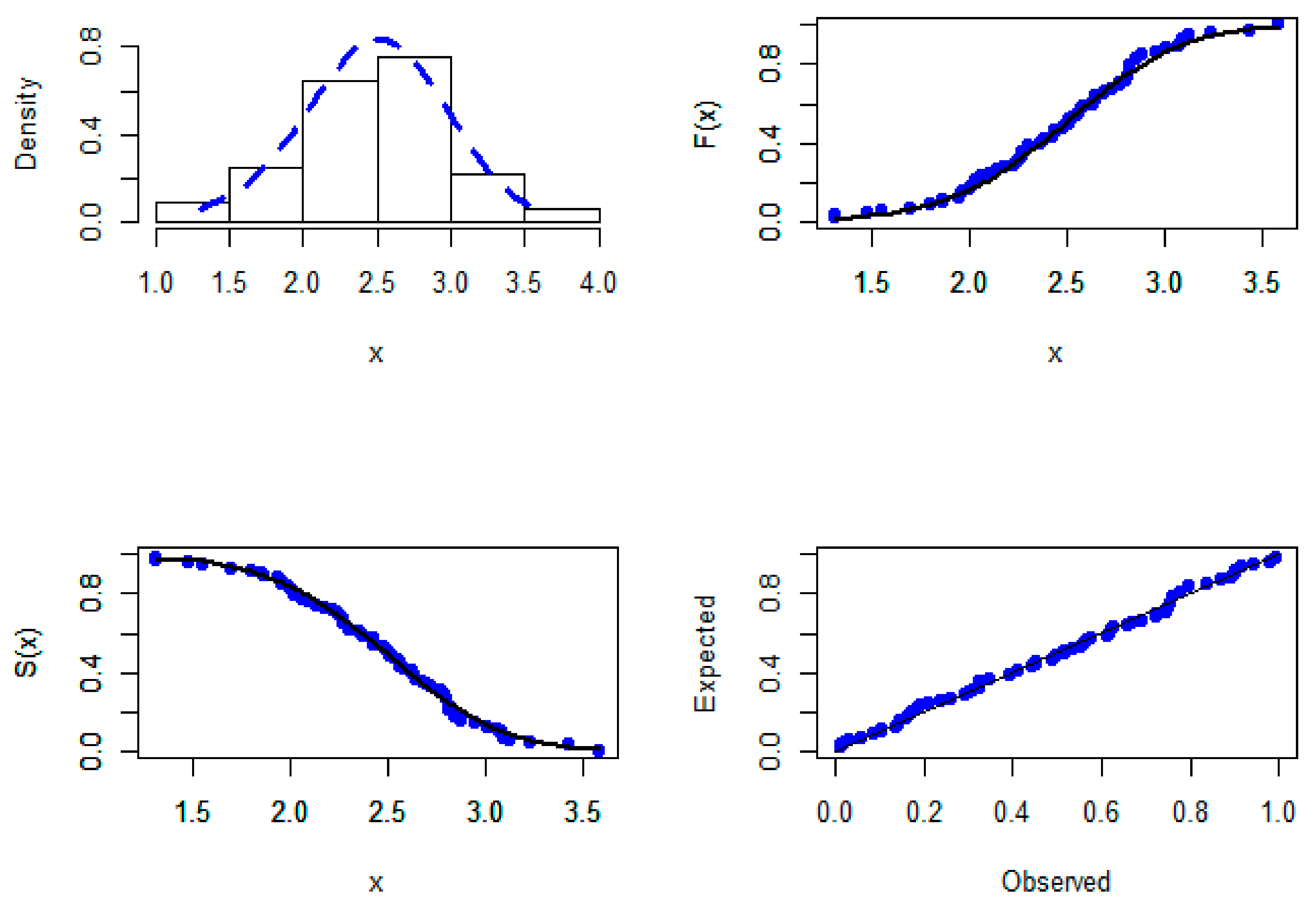
. The OEHLE distribution provides close fits than other competing models. Figure 3 shows the fitted functions of the OEHLE model for gauge lengths data, using the estimates in Table 3. Furthermore, the fitted PDFs for the OEHLE distribution and the best five competing models are displayed in Figure 4.

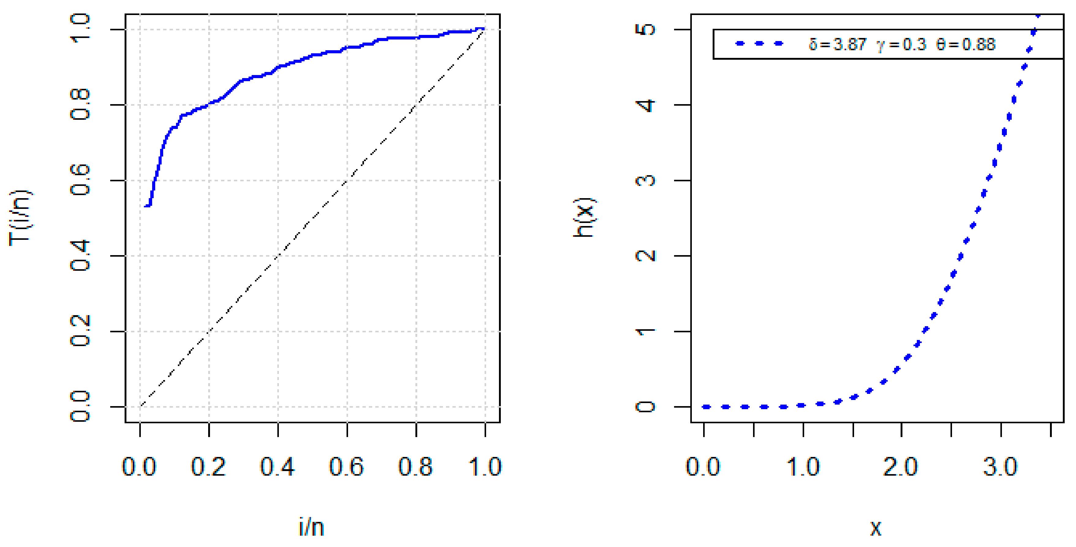
The total time on test (TTT) plot can be utilized to identify the behaviour of the HRF of the data. When we obtain a diagonal line, we conclude that the data have a constant HRF. The concave TTT plot means that the data have an increasing HRF, whereas a convex TTT plot reveals that the data have a decreasing HRF. Further, it can be concave and then convex or convex and then concave, proving that the data have a unimodal or bathtub hazard rates, respectively.

The scaled TTT plot provides a concave shape illustrating that the gauge lengths data have an increasing failure rate as displayed in Figure 5. Furthermore, the HRF plot of the OEHLE distribution for gauge lengths data, using the estimates in Table 3, is depicted in Figure 5. The increasing HRF, in Figure 5, is plotted using the estimates obtained from the data, and it indicates that the OEHLE distribution is suitable for modelling this data set.

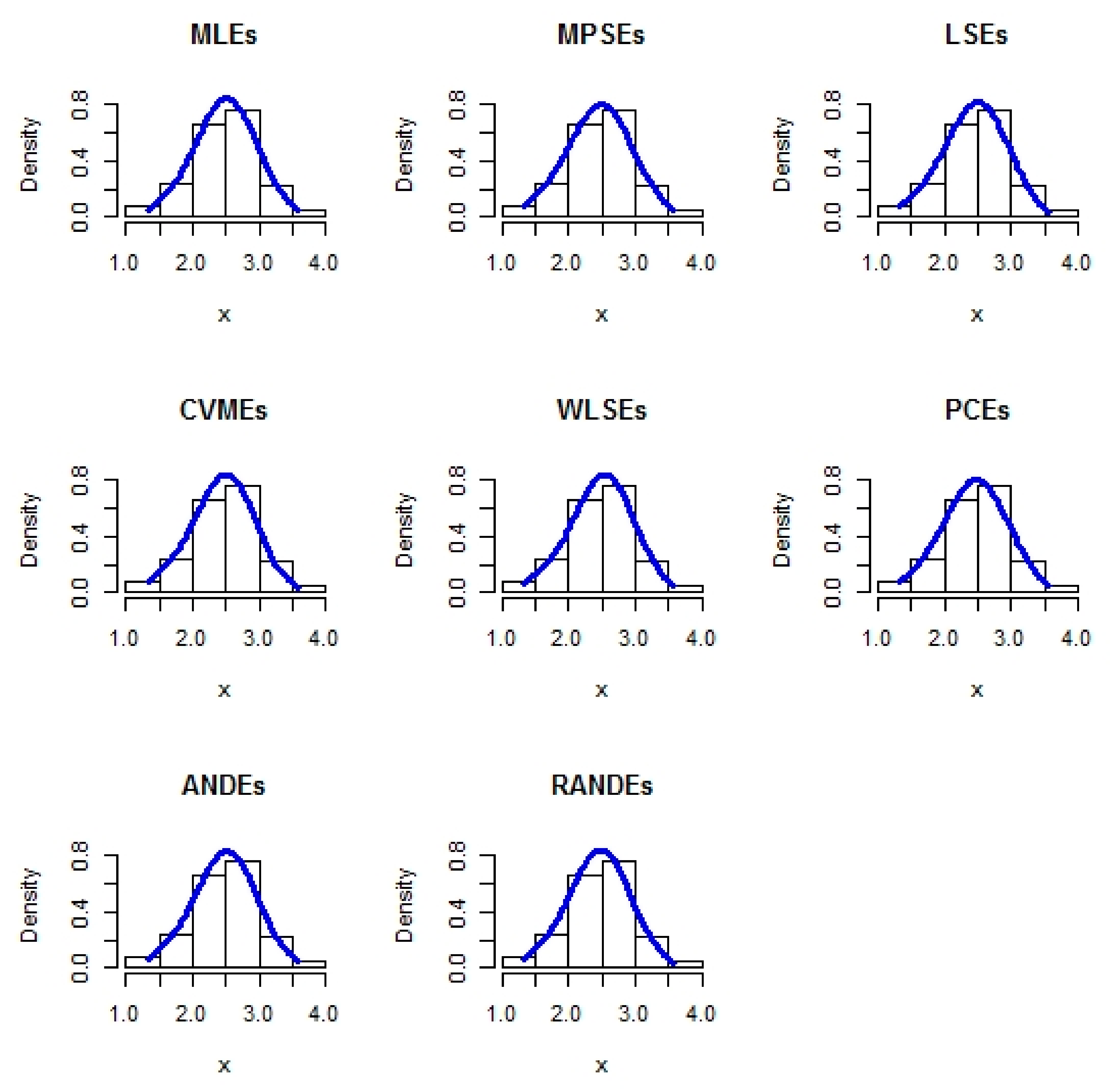
The eight estimation methods are also utilized to estimate the OEHLE parameters from the gauge lengths data. The estimates and the values of KS statistic with its $p$-value are reported in

Table 4. The estimates of the OEHLE parameters using eight estimation methods, KS and p-value for the gauge lengths data.

Model	$\widehat{\mathit{\delta }}$	$\widehat{\mathit{\gamma }}$	$\widehat{\mathit{\theta }}$	KS	p-Value
MLEs	3.8722	0.3005	0.8837	0.054549	0.980302
MPSEs	3.1774	0.2652	0.9108	0.047089	0.997130
LSEs	2.9708	0.2124	0.9809	0.042001	0.999513
CVMEs	3.0332	0.2047	0.9981	0.040502	0.999747
WLSEs	2.9358	0.1829	1.0174	0.068456	0.895546
PCEs	3.5193	0.3156	0.8657	0.044450	0.998766
ANDEs	3.4364	0.2610	0.9210	0.041639	0.999582
RANDEs	3.4685	0.2636	0.9278	0.042351	0.999439

. It is clear, from the KS and $p$-values in Table 4, that the CVMEs is recommended for estimating the OEHLE parameters for gauge length data. Furthermore, one can conclude that all eight estimation methods perform very well.

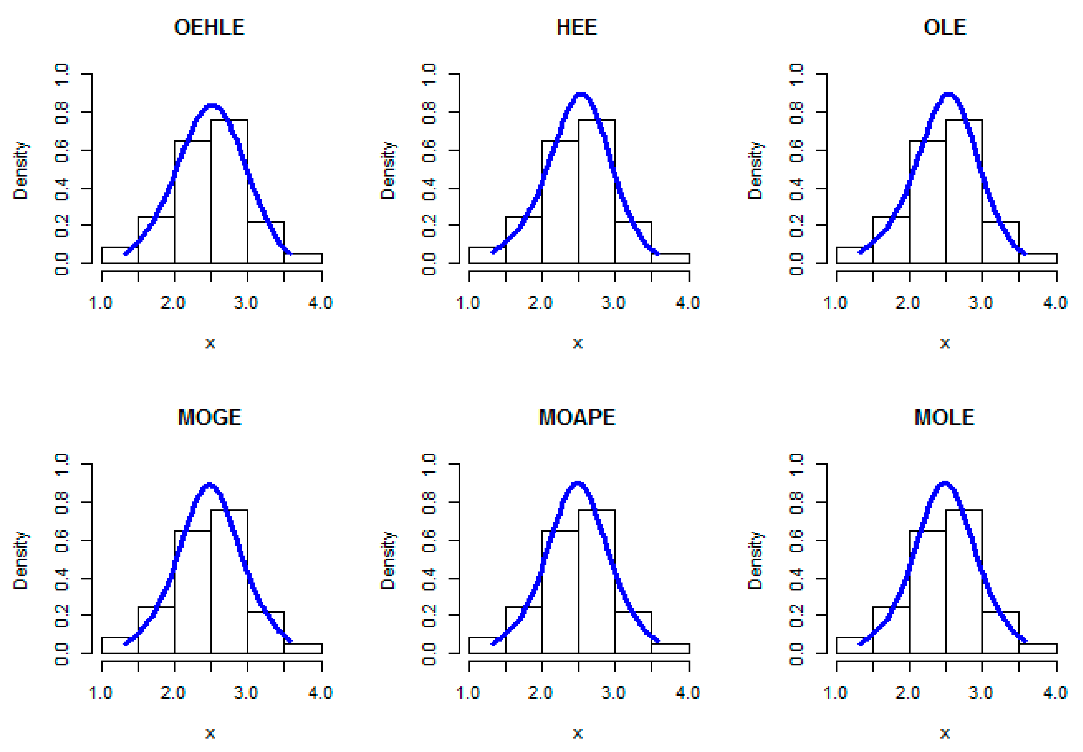
Additionally, based on the KS and $p$-values in Table 4, the performance ordering of these estimators from best to worst is CVMEs, ANDEs, LSEs, RANDEs, PCEs, MPSEs, MLEs and WLSEs for the gauge lengths data. A visual comparison of the histogram of the gauge lengths data with the fitted PDFs forms the eight estimation methods displayed in Figure 6. This visual comparison supports the results in Table 4, that all estimation methods perform very well.

5. Conclusions

In this paper, we discussed the estimation of the odd exponentiated half-logistic exponential parameters using eight frequentist estimation methods, namely the maximum likelihood, least squares, maximum product of spacing, Cramér–von-Mises, weighted least squares, percentiles, Anderson–Darling, and right-tail Anderson–Darling.

Since the theoretical comparison between these frequentist estimation methods is not feasible, hence we conducted a detailed simulation study to compare them in terms of mean square error of the estimates, average absolute biases, mean relative estimates, and the total absolute relative error of the parameters. The results illustrate that all classical estimators perform very well and their performance ordering, based on overall ranks, from best to worst, is the maximum product of spacing, maximum likelihood, Anderson–Darling, percentiles, weighted least squares, least squares, right-tail Anderson–Darling, and Cramér–von-Mises estimators for all studied cases. We can also conclude that the MPSEs outperform all other estimators with an overall score of 35. Therefore, based on our study, we can confirm the superiority of MPSEs and MLEs, with respective overall scores of 35 and 76, for the OEHLE distribution. The practical importance of the odd exponentiated half-logistic exponential distribution is illustrated by a real-life data from the engineering field. The odd exponentiated half-logistic exponential distribution can provide better fits for the analysed data than some other competing exponential distributions such as the Harris extended exponential, odd Lomax exponential, Marshall–Olkin generalised exponential, Marshall–Olkin alpha-power exponential, Marshall–Olkin logistic exponential, Marshall–Olkin Nadarajah–Haghighi, modified exponential, beta generalised exponential, beta exponential, exponentiated exponential, and exponential distributions. Furthermore, the odd exponentiated half-logistic exponential distribution can be used in modelling data with increasing, decreasing, and bathtub failure rates encountered in several sciences such as medicine, reliability, economics, insurance, and life testing, among others.

References

- Gupta, R.D.; Kundu, D. Exponentiated exponential family: An alternative to gamma and Weibull distributions. Biom. J. 2001, 43, 117–130. [Google Scholar] [CrossRef]
- Pinho, L.G.B.; Cordeiro, G.M.; Nobre, J.S. The Harris extended exponential distribution. Commun. Stat. Theory Methods 2015, 44, 3486–3502. [Google Scholar] [CrossRef]
- Jones, M.C. Families of distributions arising from distributions of order statistics. Test 2004, 13, 1–43. [Google Scholar] [CrossRef]
- Khan, M.S.; King, R.; Hudson, I.L. Transmuted generalized exponential distribution: A generalization of the exponential distribution with applications to survival data. Commun. Stat. Simul. Comput. 2017, 46, 4377–4398. [Google Scholar] [CrossRef]
- Mahdavi, A.; Kundu, D. A new method for generating distributions with an application to exponential distribution. Commun. Stat. Theory Methods 2017, 46, 6543–6557. [Google Scholar] [CrossRef]
- Nassar, M.; Afify, A.Z.; Shakhatreh, M. Estimation methods of alpha power exponential distribution with applications to engineering and medical data. Pak. J. Stat. Oper. Res. 2020, 16, 149–166. [Google Scholar] [CrossRef]
- Afify, A.Z.; Cordeiro, G.M.; Yousof, H.M.; Alzaatreh, A.; Nofal, Z.M. The Kumaraswamy transmuted-G family of distributions: Properties and applications. J. Data Sci. 2016, 14, 245–270. [Google Scholar]
- Rasekhi, M.; Alizadeh, M.; Altun, E.; Hamedani, G.G.; Afify, A.Z.; Ahmad, M. The modified exponential distribution with applications. Pak. J. Stat. 2017, 33, 383–398. [Google Scholar]
- Mansoor, M.; Tahir, M.H.; Cordeiro, G.M.; Provost, S.B.; Alzaatreh, A. The Marshall-Olkin logistic-exponential distribution. Commun. Stat. Theory Methods 2017, 48, 220–234. [Google Scholar] [CrossRef]
- Aldahlan, M.A. A new three-parameter lifetime distribution: Properties and applications. Int. J. Innov. Sci. Math. 2019, 7, 54–66. [Google Scholar]
- Nassar, M.; Kumar, D.; Dey, S.; Cordeiro, G.M.; Afify, A.Z. The Marshall-Olkin alpha power family of distributions with applications. J. Comput. Appl. Math. 2019, 351, 41–53. [Google Scholar] [CrossRef]
- Alizadeh, M.; Afify, A.Z.; Eliwa, M.S.; Ali, S. The odd log-logistic Lindley-G family of distributions: Properties, Bayesian and non-Bayesian estimation with applications. Comput. Stat. 2020, 35, 281–308. [Google Scholar] [CrossRef]
- Afify, A.Z.; Mohamed, O.A. A new three-parameter exponential distribution with variable shapes for the hazard rate: Estimation and applications. Mathematics 2020, 8, 135. [Google Scholar] [CrossRef] [Green Version]
- Afify, A.Z.; Zayed, M.; Ahsanullah, M. The extended exponential distribution and its applications. J. Stat. Theory Appl. 2018, 17, 213–229. [Google Scholar] [CrossRef] [Green Version]
- Afify, A.Z.; Altun, E.; Alizadeh, M.; Ozel, G.; Hamedani, G.G. The odd exponentiated half-logistic-G family: Properties, characterizations and applications. Chilean J. Stat. 2017, 8, 65–91. [Google Scholar]
- Kundu, D.; Raqab, M.Z. Generalized Rayleigh distribution: Different methods of estimations. Comput. Stat. Data Anal. 2005, 49, 187–200. [Google Scholar] [CrossRef]
- Mazucheli, J.; Louzada, F.; Ghitany, M. Comparison of estimation methods for the parameters of the weighted Lindley distribution. Appl. Math. Comput. 2013, 220, 463–471. [Google Scholar] [CrossRef]
- Dey, S.; Kumar, D.; Ramos, P.L.; Louzada, F. Exponentiated Chen distribution: Properties and estimation. Commun. Stat. Simul. Comput. 2017, 46, 8118–8139. [Google Scholar] [CrossRef]
- Nassar, M.; Afify, A.Z.; Dey, S.; Kumar, D. A new extension of Weibull distribution: Properties and different methods of estimation. J. Comput. Appl. Math. 2018, 336, 439–457. [Google Scholar] [CrossRef]
- Nassar, M.; Dey, S.; Kumar, D. A new generalization of the exponentiated Pareto distribution with an application. Am. J. Math. Manag. Sci. 2018, 37, 217–242. [Google Scholar] [CrossRef]
- Aldahlan, M.A. Different methods of estimation for the parameters of half logistic Lomax distribution. Appl. Math. Sci. 2019, 13, 201–208. [Google Scholar] [CrossRef] [Green Version]
- Sen, S.; Afify, A.Z.; Al-Mofleh, H.; Ahsanullah, M. The quasi xgamma-geometric distribution with application in medicine. Filomat 2019, 33, 5291–5330. [Google Scholar] [CrossRef] [Green Version]
- Afify, A.Z.; Nassar, M.; Cordeiro, G.M.; Kumar, D. The Weibull Marshall–Olkin Lindley distribution: Properties and estimation. J. Taibah Univ. Sci. 2020, 14, 192–204. [Google Scholar] [CrossRef]
- Nassar, M.; Afify, A.Z.; Shakhatreh, M.; Dey, S. On a new extension of Weibull distribution: Properties, estimation, and applications to one and two causes of failures. Qual. Reliab. Engng. Int. 2020, 1–25. [Google Scholar] [CrossRef]
- Cheng, R.; Amin, N. Maximum Product of Spacings Estimation with Application to the Lognormal Distribution; Mathematical Report 79-1; University of Wales: Cardiff, UK, 1979. [Google Scholar]
- Cheng, R.; Amin, N. Estimating parameters in continuous univariate distributions with a shifted origin. J. R. Stat. Soc. Ser. B Methodol. 1983, 45, 394–403. [Google Scholar] [CrossRef]
- Ranneby, B. The maximum spacing method: An estimation method related to the maximum likelihood method. Scand. J. Stat. 1984, 11, 93–112. [Google Scholar]
- Swain, J.; Venkatraman, S.; Wilson, J. Least squares estimation of distribution function in Johnsons translation system. J. Stat. Comput. Simul. 1988, 29, 271–297. [Google Scholar] [CrossRef]
- Macdonald, P. Comment on “An estimation procedure for mixtures of distribution” by Choi and Bulgren. J. R. Stat. Soc. Ser. B Methodol. 1971, 33, 326–329. [Google Scholar]
- Luceno, A. Fitting the generalized Pareto distribution to data using maximum goodness-of-fit estimators. Comput. Stat. Data Anal. 2006, 51, 904–917. [Google Scholar] [CrossRef]
- Kao, J. Computer methods for estimating Weibull parameters in reliability studies. IRE Reliab. Qual. Control 1958, 13, 15–22. [Google Scholar] [CrossRef]
- Kao, J. A graphical estimation of mixed Weibull parameters in life testing electron tube. Technometrics 1959, 1, 389–407. [Google Scholar] [CrossRef]
- Kundu, D.; Raqab, M.Z. Estimation of R = P(Y < X) for three parameter Weibull distribution. Stat. Probab. Lett. 2009, 79, 1839–1846. [Google Scholar]
- Afify, A.Z. Three-parameter exponential distribution: Estimation and applications. J. Stat. Theory Appl. 2020. To Appear. [Google Scholar]
- Ristić, M.M.; Kundu, D. Marshall-Olkin generalized exponential distribution. Metron 2015, 73, 317–333. [Google Scholar] [CrossRef]
- Lemonte, A.J.; Cordeiro, G.M.; Moreno-Arenas, G. A new useful three-parameter extension of the exponential distribution. Statistics 2016, 50, 312–337. [Google Scholar] [CrossRef]
- Barreto-Souza, W.; Santos, A.H.; Cordeiro, G.M. The beta generalized exponential distribution. J. Stat. Comput. Simul. 2010, 80, 159–172. [Google Scholar] [CrossRef] [Green Version]