Optimal Sliced Latin Hypercube Designs with Slices of Arbitrary Run Sizes

Abstract

Sliced Latin hypercube designs (SLHDs) are widely used in computer experiments with both quantitative and qualitative factors and in batches. Optimal SLHDs achieve better space-filling property on the whole experimental region. However, most existing methods for constructing optimal SLHDs have restriction on the run sizes. In this paper, we propose a new method for constructing SLHDs with arbitrary run sizes, and a new combined space-filling measurement describing the space-filling property for both the whole design and its slices. Furthermore, we develop general algorithms to search for the optimal SLHD with arbitrary run sizes under the proposed measurement. Examples are presented to illustrate that effectiveness of the proposed methods.

1. Introduction

Computer experiments are becoming increasingly significant in many fields, such as finite element analysis and computational fluid dynamics. Latin hypercube designs (LHDs) [1] are widely used in computer experiments because of their optimal univariate uniformity. A design with n runs and q factors is called an LHD; if the design is projected onto any one dimension, there is precisely one point lying within one of the n intervals $(0,1/n],(1/n,2/n],\cdots ,\left(\right(n-1)/n,1]$. Such an LHD is said to have optimal univariate uniformity. Sliced Latin hypercube designs (SLHDs) are LHDs that can be partitioned into some LHD slices [2], which means that the SLHDs have the optimal univariate uniformity for both the whole design and their slices. In [3], a central limit theorem for SLHDs is proposed. SLHDs are popular for computer experiments with both qualitative and quantitative variables; see [4,5,6] and the references therein. Each slice of an SLHD can be used under one level-combination of the qualitative factors. However, the original SLHDs and almost all existing methods for constructing variants of SLHDs require that the run sizes of each slice are equal; see [7,8,9,10].

An SLHD is called desirable if its design points are well spread out for both the whole design and its slices. Randomly generated SLHDs usually have a poor space-filling property in the entire experimental region, i.e., randomly generated SLHDs may not be desirable. There are many methods that aim to improve the space-filling property of an SLHD. For instance, the method proposed by [11] can be used to generate an optimal clustered-sliced Latin hypercube design (OCSLHD) which has a good space-filling property in the whole experimental region. In a multi-fidelity computer experiment, each slice of an OCSLHD can be used for each accuracy of the computer code [11]. Generally, we want to use more design points for the lower-accuracy experiments than those of the higher-accuracy experiments, since the lower the accuracy is, the faster it runs [12,13]. However, many existing methods for constructing optimal SLHDs can only generate SLHDs with equal run sizes of each slice, e.g., [11,14,15]. To overcome this restriction, we need a method that can construct SLHDs with slices of arbitrary run sizes, and with a good space-filling property over the whole experimental region. For example, the authors in [16] gave flexible sliced designs, but such designs are not LHDs. The method given in [17] provided SLHDs with unequal batch sizes, but this type of design only accommodates two different run sizes. A random sampling procedure for constructing flexible SLHDs is given in [18]. However, the design is constructed by the procedure with slow efficiency if the design has large design points. An algorithm is proposed in [19] to construct a midpoint SLHD with unequal run sizes, which has the fast efficiency for constructing the design, but such a design is difficult to be used as an initial design to search for the optimal design. Firstly, we are interested in constructing randomized SLHDs with slices of arbitrary run sizes, and we want to have more flexible elements to construct the design. Secondly, we can exchange some elements of different slices, and the design still keeps the sliced structure, while the elements in each slice of the design are fixed in [19]. We can consider proposing a method that is easily adapted to generate the optimal design.

In this paper, we propose an improved method to construct SLHDs with slices of arbitrary run sizes, which are called flexible sliced Latin hypercube designs (FSLHDs). The new construction method can be easily adapted to generate the optimal design. Furthermore, we provide a combined space-filling measurement (CSM) to describe the space-filling properties of both the whole design and each of slices. Based on an optimization algorithm called the enhanced stochastic evolutionary algorithm (ESE), we propose a sliced ESE (SESE) algorithm to find the optimal FSLHDs. We further develop an efficient two-part algorithm to improve the efficiency in generating space-filling FSLHDs with large runs and factors. The generated optimal FSLHDs have three attractive features: (i) arbitrary run sizes of all slices, (ii) optimal univariate uniformity in the whole design and each slice, and (iii) good space-filling property in the experimental region. We believe that they are suitable for many multi-fidelity computer experiments in practice.

The remainder of this paper is organized as follows. The construction of FSLHDs is provided in Section 2. In Section 3, an CSM is given to describe the space-filling properties of both the whole design and each of slices, and then we develop an SESE algorithm to obtain optimal FSLHDs based on the CSM and a two-part algorithm to improve efficiency. Some simulation results are illustrated in Section 4. Section 5 provides some discussions. Section 6 concludes this paper. The corresponding codes for Section 2, Section 3 and Section 4 can be found in the Supplementary Materials.

2. Construction of SLHDs with Slices of Arbitrary Run Sizes

For a real number a, let $\lceil a\rceil$ denote the smallest integer not smaller than a. Given u positive integers $n_1,\cdots ,n_u$, let $n={\sum }_{i=1}^u{n}_i$ and let $L=\mathrm{lcm}(n_1,\cdots ,n_u,n)$ be the least common multiple of $n_1,\cdots ,n_u$, and n. Suppose that $\mathrm{FSLHD}(n_1,\cdots ,n_u;u,q)$ is an FSHLD with u slices of run sizes $n_1,\cdots ,n_u$ and q factors. Each column of the FSLHD is generated independently by the following algorithm:

Step 1. 

Let $H^i=⌀$ for $i=1,\cdots ,u$, and $R_0=⌀$.

Step 2. 

For $j=1,\cdots ,n$, let $R_{j,0}=R_{j-1}\bigcup \left\{j\right\}$ and calculate

$${\theta }_j={\sum }_{i=1}^u\left(\lceil n_i(j+1)/n\rceil -\lceil n_{i}j/n\rceil \right).$$

If ${\theta }_j>0$, for $k=1,\cdots ,{\theta }_j$, let l denote the kth smallest integer of the set $\left\{p\right|\lceil n_p(j+1)/n\rceil -\lceil n_{p}j/n\rceil =1\}$ and $r=min\left\{r\right|\lceil n_{l}r/n\rceil =\lceil n_{l}j/n\rceil ,r\in R_{j,k-1}\}$ add r to $H^l$ and let $R_{j,k}=R_{j,k-1}\setminus \left\{r\right\}$. Let $R_j=R_{j,{\theta }_j}$ and go to the next j.

Step 3. 

For $i=1,\cdots ,u$, generate a vector ${\mathit{h}}^i$ by randomly permuting $H^i$.

Step 4. 

For $i=1,\cdots ,u$, calculate ${\mathit{m}}^i=L{\mathit{h}}^i/n$, where ${\mathit{m}}^i=(m_1^i,\cdots ,m_{n_i}^i)$. Combine ${\mathit{m}}^1,\cdots ,{\mathit{m}}^u$ to obtain an n-dimensional column vector $\mathit{m}={(m_1,\cdots ,m_n)}^T$, then let ${\mathit{d}}^i={(d_1^i,\cdots ,d_{n_i}^i)}^T$ be constructed by

$$d_s^i=(m_s^i-{\epsilon }_s^i)/L,s=1,\cdots ,n_i,$$

(1)

where ${\epsilon }_s^i\sim U(0,1)$. Combine ${\mathit{d}}^1,\cdots ,{\mathit{d}}^u$ to obtain an n-dimensional column vector $\mathit{d}={(d_1,\cdots ,d_n)}^T$, and $\mathit{d}$ is one column of the design.

In the above algorithm, $\mathit{m}$ is called a column of the flexible sliced Latin hypercube (FSLH). The following theorem shows that both the whole FSLHD and its slices are LHDs.

Theorem 1.

Let $\mathit{d}={(d_1,\cdots ,d_n)}^T$ denote an arbitrary column of FSLHD($n_1,\cdots ,n_u;u,q$) generated by the above method. Let ${\mathit{d}}^1,\cdots ,{\mathit{d}}^u$ denote each slice. For $i=1,\cdots ,u$, let $t^i=L/n_i$ and $t^{\prime }=L/n$.

(i) Precisely, one point of $\mathit{d}={(d_1,\cdots ,d_n)}^T$ lies within one of the n intervals $(0,1/n],(1/n,2/n],\cdots ,\left(\right(n-1)/n,1]$.

(ii) Precisely, one point of ${\mathit{d}}^i=(d_1^i,\cdots ,d_{n_i}^i)$ lies within one of the $n_i$ intervals $(0,1/n_i],(1/n_i,2/n_i]$,$\cdots ,((n_i-1)/n_i,1]$.

Proof. 

(i) Combine ${\mathit{h}}^1,\cdots ,{\mathit{h}}^u$ to obtain $\mathit{h}={(h_1,\cdots ,h_n)}^T$ that is a permutation of $\{1,\cdots ,n\}$. Combine ${\mathit{m}}^1,\cdots ,{\mathit{m}}^u$ to obtain $\mathit{m}={(m_1,\cdots ,m_n)}^T$. Therefore, $\mathit{m}=L\mathit{h}/n$. For $t^{\prime }=L/n$ because $\lceil \mathit{m}/t^{\prime }\rceil =\lceil (L\mathit{h}/n)/t^{\prime }\rceil =\lceil \mathit{h}\rceil$, $\lceil \mathit{m}/t^{\prime }\rceil$ is a permutation of $\{1,\cdots ,n\}$. Therefore, precisely one point of $\mathit{d}={(d_1,\cdots ,d_n)}^T$ lies within one of the n intervals $(0,1/n],(1/n,2/n],\cdots ,\left(\right(n-1)/n,1]$.

(ii) According to Step 2, for $i=1,\cdots ,u$, it is clear that $card\left(H^i\right)={\sum }_{j=1}^n(\lceil n_i(j+1)/n\rceil -\lceil n_{i}j/n\rceil )=\lceil n_i(n+1)/n\rceil -\lceil n_i/n\rceil =n_i$, and for $j=1,\cdots ,n$, $\lceil n_{i}j/n\rceil <\lceil n_i(j+1)/n\rceil$. For any i, j, there is an integer $h\in H^i$ that satisfies $\lceil n_{i}h/n\rceil =\lceil n_{i}j/n\rceil$. Therefore, we have $\left\{m\right|m=\lceil n_{i}h/n\rceil ,h\in H^i\}=\{1,\cdots ,n_i\}$, which means that $\lceil n_i{\mathit{h}}^i/n\rceil$ is a permutation of $\{1,\cdots ,n_i\}$. Since ${\mathit{m}}^i=L{\mathit{h}}^i/n$, we have $\lceil {\mathit{m}}^i/t^i\rceil =\lceil (L{\mathit{h}}^i/n)/(L/n_i)\rceil =\lceil n_i{\mathit{h}}^i/n\rceil$. Thus, $\lceil {\mathit{m}}^i/t^i\rceil$ is a permutation of $\{1,\cdots ,n_i\}$. Therefore, precisely one point of ${\mathit{d}}^i$ lies within one of the $n_i$ intervals $(0,1/n_i],(1/n_i,2/n_i],\cdots ,((n_i-1)/n_i,1]$. □

We give an example to illustrate the process of the above method.

Example 1.

Consider$n_1=3$,$n_2=4$,$n_3=5$,$u=3$,$n=12$, and $L=60$.

Step 1. 

$H^1=H^2=H^3=R_0=\varnothing$.

Step 2. 

Calculate $({\theta }_1,\cdots ,{\theta }_n)=(0,1,1,2,0,1,1,1,2,0,0,3)$. For $j=1$, then $R_{1,0}=\left\{1\right\}$, since ${\theta }_1=0$, we obtain $R_1=R_{1,0}=\left\{1\right\}$. For $j=2$, $R_{2,0}=R_1\cup \left\{2\right\}=\{1,2\}$, ${\theta }_2=1$, only an integer $l=3$ satisfies $\lceil n_l(j+1)/n\rceil -\lceil n_{L}j/n\rceil =1$, and $r=$ min$\left\{r\right|\lceil n_{3}r/n\rceil =\lceil n_{3}j/n\rceil$, $r\in R_{2,0}\}=$ min$\{1,2\}=1$. Hence, we add $r=1$ to $H^3$, $R_{2,1}=R_{2,0}\setminus \left\{1\right\}=\left\{2\right\}$, and $R_2=R_{2,1}=\left\{2\right\}$. For $j=3$, $R_{3,0}=R_2\cup \left\{3\right\}=\{2,3\}$, ${\theta }_3=1$, only an integer $l=2$ satisfies $\lceil n_2(j+1)/n\rceil -\lceil n_{2}j/n\rceil =1$, and $r=$ min$\left\{r\right|\lceil n_{2}r/n\rceil =\lceil n_{2}j/n\rceil$, $r\in R_{3,0}\}=$ min$\{2,3\}=2$. Therefore, we add $r=2$ to $H^2$, $R_{3,1}=R_{3,0}\setminus \left\{2\right\}=\left\{3\right\}$, and $R_3=R_{3,1}=\left\{3\right\}$. After passing all j, we can get $R_{12}=\varnothing$, $H^1=\{3,7,10\}$, $H^2=\{2,5,8,11\}$, and $H^3=\{1,4,6,9,12\}$.

Step 3. 

We get ${\mathit{h}}^1=(10,7,3)$, ${\mathit{h}}^2=(5,8,2,11)$, and ${\mathit{h}}^3=(6,9,12,1,4)$ by randomly permuting $H^1$, $H^2$, and $H^3$.

Step 4. 

We obtain ${\mathit{m}}^1=(50,35,15)$, ${\mathit{m}}^2=(25,40,10,55)$, and ${\mathit{m}}^3=(30,45,60,5,20)$. Then, ${\mathit{d}}^i={(d_1^i,\cdots ,d_{n_i}^i)}^T$ is constructed through $d_s^i=(m_s^i-{\epsilon }_s^i)/60$, where $i=1,\cdots ,3$, $s=1,\cdots ,n_i$, and ${\epsilon }_s^i\sim U(0,1)$. Thus, we obtain an arbitrary column $\mathit{d}={(d_1,\cdots ,d_n)}^T$ of the design.

3. Optimal SLHDs with Slices of Arbitrary Run Sizes

Given $n_1,\cdots ,n_u,u,q$, a number of possible FSLHDs can be generated through the proposed method in Section 2. Among such FSLHDs, we can find the optimal FSLHD through a given space-filling criterion. We first propose a combined space-filling measurement (CSM) to evaluate space-filling property of FSLHD in Section 3.1. Then, to keep the structure of the design during the optimization process, three methods are proposed to change position of the elements in one column in Section 3.2. Finally, we present a sliced ESE algorithm to optimize FSLHD in Section 3.3. An efficient two-part algorithm for generating the space-filling FSLHD is given in Section 3.4.

3.1. A Combined Space-Filling Measurement for FSLHDs

Various space-filling criteria are used to evaluate the LHDs, such as the maximin distance criterion [20,21,22,23], the ${\varphi }_t$ criterion [24,25,26,27], and the centered $L_2$-discrepancy (${\mathrm{C}D}_2$) criterion [28,29]. All the space-filling criteria can be extended to describe the space-filling property of the FSLHDs. We mainly focus on the ${\varphi }_t$ criterion, which is an attractive extension of maximin distance criterion.

The maximin distance criterion is a popular space-filling criterion introduced in [20]. Let $\mathit{D}={[{\mathit{x}}_1,\cdots ,{\mathit{x}}_n]}^T$ denote a design matrix with n runs and q factors, where each row ${\mathit{x}}_i^T=(x_{i1},\cdots ,x_{iq})$ is a design point and each column is a factor with $i=1,\cdots ,n$. A maximin distance design is generated by maximizing the minimum inter-site distance, which is expressed as

$$\underset{\forall 1\le i,j\le n,i\ne j}{min}{d}_{ij},$$

(2)

where $d_{ij}$ is the distance between the design points ${\mathit{x}}_i$ and ${\mathit{x}}_j$ given by:

$$d_{ij}={\left(\sum _{k=1}^q{|x_{ik}-x_{jk}|}^m\right)}^{1/m},m=1\mathrm{or}2.$$

(3)

Here, $m=1$ and $m=2$ are the rectangular and Euclidean distances, respectively. In this article, we use the Euclidean distance. An extension of the maximin distance criterion [24] is given by

$${\varphi }_t={\left(\sum _{1\le i<j\le n}{\left(d_{ij}\right)}^{-t}\right)}^{1/t},$$

(4)

where t is a positive integer. It is obvious that as $t⟶\infty$, minimizing (4) is equivalent to maximizing (2). The calculation of ${\varphi }_t$ is simpler compared with the maximin distance criterion.

We search for an optimal design by minimizing ${\varphi }_t$, i.e.,

$${\mathit{D}}^{*}=arg\underset{\mathit{D}}{min}{\varphi }_t\left(\mathit{D}\right).$$

(5)

Suppose that $\mathit{D}$ is the design matrix of an $\mathrm{FSLHD}(n_1,\dots ,n_u;u,q)$. For $i=1,\dots ,u$, let ${\mathit{D}}^{\left(i\right)}$ denote each slice of $\mathit{D}$. We need to consider both the space-filling properties of the whole FSLHD and that of its slices. Consequently, our goal is to find a maximin FSLHD that minimizes ${\varphi }_t\left(\mathit{D}\right)$ for the entire design as well as ${\varphi }_t\left({\mathit{D}}^{\left(i\right)}\right)$ for each slice of $\mathit{D}$ ($i=1,\dots ,u$). This is a multi-objective optimization problem. It is a common method in a multi-objective problem to use a weighted average of all individual objectives. It motivates us to develop a combined space-filling measurement (CSM) as follows:

$${\varphi }_{\mathrm{CSM}}\left(\mathit{D}\right)=w{\varphi }_t\left(\mathit{D}\right)+(1-w)\left(\sum _{i=1}^u{\lambda }_i{\varphi }_t\left({\mathit{D}}^{\left(i\right)}\right)\right),$$

(6)

where ${\lambda }_i=n_i/n$, ${\sum }_{i=1}^u{\lambda }_i=1$, and $w\in (0,1)$. Since run sizes of slices are $n_1,\dots ,n_u$, respectively, it makes sense that we take the weight of each slice to be ${\lambda }_i=n_i/n$, for $i=1,\dots ,u$. The weight w is selected flexibly. The space-filling property of the whole FSLHD is more important, hence we set $w=1/2$ in general. We can define a maximin distance FSLHD with respect to the CSM as the one that minimizes (6).

Note that other space-filling criteria can also evaluate the FSLHD. For instance, we can obtain an uniform FSLHD by minimizing a similar CSM given by

$$\begin{array}{c}\hfill {\varphi }_{\mathrm{CSM}}\left(\mathit{D}\right)=w{\varphi }_{{\mathrm{CD}}_2}\left(\mathit{D}\right)+(1-w)\left(\sum _{i=1}^u{\lambda }_i{\varphi }_{{\mathrm{CD}}_2}\left({\mathit{D}}^{\left(i\right)}\right)\right),\end{array}$$

(7)

where ${\varphi }_{{\mathrm{CD}}_2}$ is the centered $L_2$-discrepancy defined as

$$\begin{array}{cc}\hfill {\varphi }_{{\mathrm{CD}}_2}=& \left({\left(\frac{13}{12}\right)}^2-\frac{2}{n}\sum _{i=1}^n\prod _{k=1}^q\left(1+\frac{1}{2}|x_{ik}-0.5|-|x_{ik}{-0.5|}^2\right)\right.\hfill \\ \hfill & {\left.+\frac{1}{n^2}\sum _{i=1}^n\sum _{j=1}^n\prod _{k=1}^q\left(1+\frac{1}{2}|x_{ik}-0.5|+\frac{1}{2}|x_{jk}-0.5|-|x_{ik}-x_{jk}|\right)\right)}^{1/2}\hfill \end{array}$$

(8)

proposed in [28].

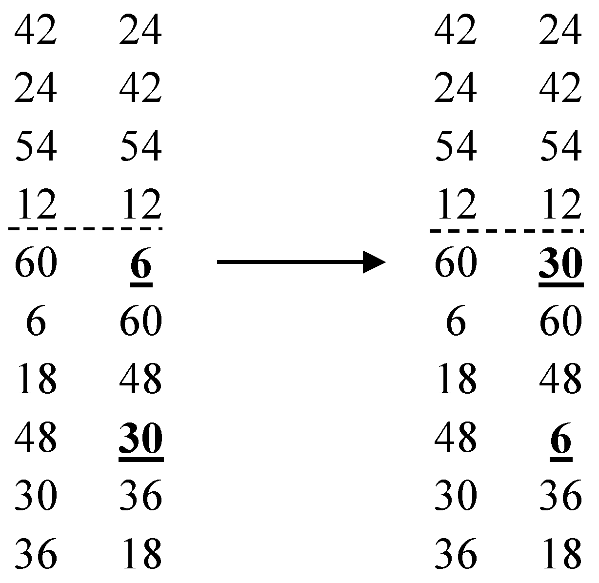
3.2. Exchange Procedures for FSLHDs

In the literature, some optimization algorithms have been widely used to construct an optimal LHD. They utilize an exchange procedure to iteratively search for the optimal LHD in the design space. In this way, two randomly selected elements in an arbitrary column of an LHD are exchanged to generate a new design. The exchange procedure for an FSLHD is more complex since the design should keep the sliced structure. In this subsection, in the optimization process of an FSLHD, we present three exchange procedures to generate a neighbour of the design which do not change the sliced structure of the design. A  neighbour of an FSLH corresponds to a neighbour of an FSLHD. Let $\mathit{M}$ be the FSLH($n_1,\cdots ,n_u;u,q$) constructed in Section 2. Let ${\mathit{M}}_{\mathrm{N}}$ denote a neighbour of an FSLH and let ${\mathit{D}}_{\mathrm{N}}$ denote a neighbour of an FSLHD.

3.2.1. The Within-Slice Exchange Procedure

Given an FSLH($n_1,\cdots ,n_u;u,q$)$\left(\mathit{M}\right)$, let $n_0=0$, $r_0=0$, and $r_i={\sum }_{k=0}^i{n}_k$, for $i=1,\cdots ,u$. The within-slice exchange procedure in the ith slice of $\mathit{M}$ is to draw an ${\mathit{M}}_{\mathrm{N}}$ by the following four steps:

Step 1. 

Randomly select a column of $\mathit{M}$.

Step 2. 

Select any two different elements $d_j,d_k$ in ith slice of the column, where $r_{i-1}+1\le j,k\le r_i$.

Step 3. 

Exchange $d_j$ and $d_k$ in the same slice.

Step 4. 

Generate ${\mathit{M}}_{\mathrm{N}}$.

After this procedure, the  neighbour design ${\mathit{M}}_{\mathrm{N}}$ still keeps the sliced structure. The within-slice exchange procedure is explained by an example about FSLH(4,6;2,2) illustrated in Figure 1.

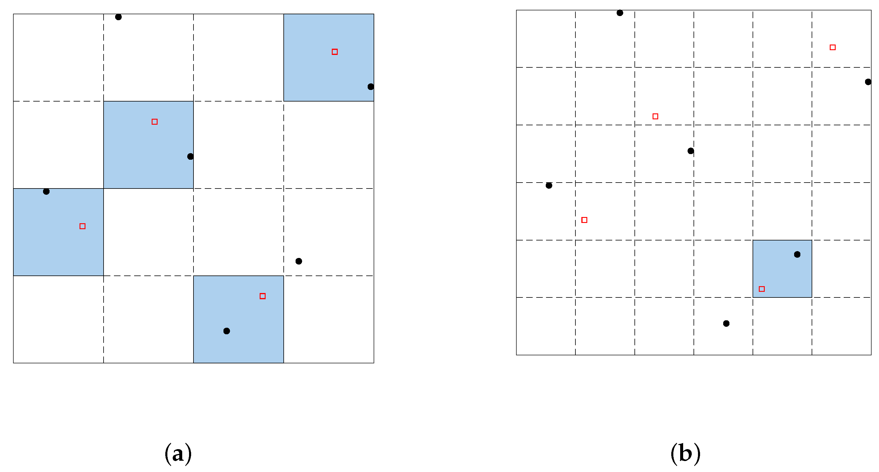
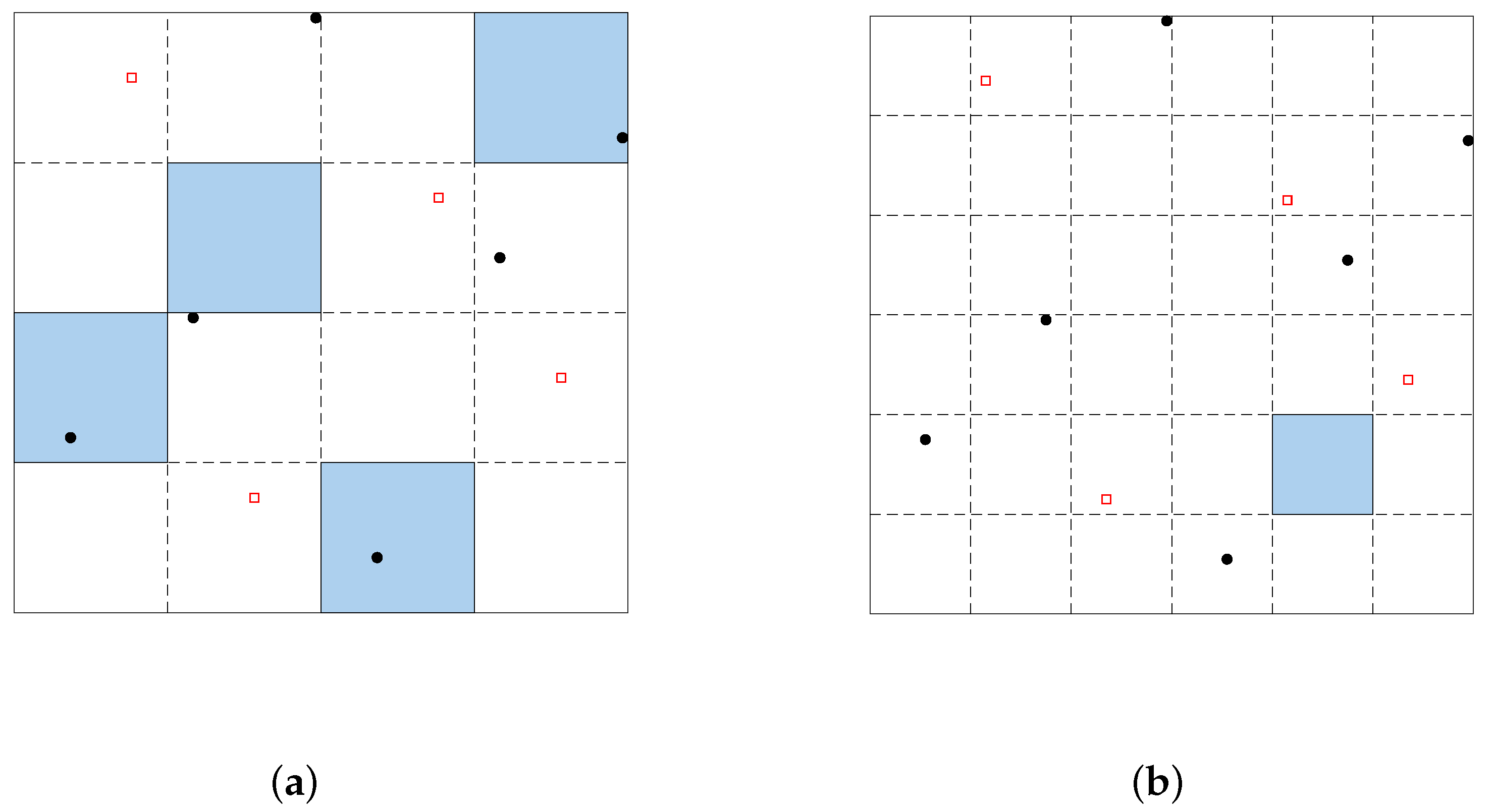
3.2.2. The Different-Slice Exchange and the Out-Slice Exchange Procedures

We first give some notations. Given an FSLH($n_1,\cdots ,n_u;u,q$)$\left(\mathit{M}\right)$, let $\mathit{M}(l:m,j)$ denote the lth to mth rows of the jth column, and $\mathit{M}(l,j)$ denotes its $(l,j)$ element. For  $i=1,\cdots ,u$, let $r_i={\sum }_{k=0}^i{n}_k$, and $B_{ij}=\mathit{M}(r_{i-1}+1:r_i,j)$ denotes ith slice in the jth column of $\mathit{M}$, where $n_0=0$, $r_0=0$. Define $E_{ij}=\{\mathit{M}(r_i+1,j),\cdots ,\mathit{M}(n,j)\}$, where $i=1,\cdots ,u-1$ and $n={\sum }_{i=1}^u{n}_i$. Let $A_L=\{1,\cdots ,L\}$ denote a set of integers from 1 to L, where $L=$ lcm$(n_1,\cdots ,n_u,n)$. Set $B=\left\{\mathit{M}\right(1,j),\cdots ,\mathit{M}(n,j\left)\right\}$. Let $C=A_L\setminus B$ denote A minus B.

It is observed that elements of each slice on an FSLHD are fixed by the construction method in Section 2. There are two situations. On the one hand, some elements in an arbitrary column of an FSLH from different slices are exchanged, and the resulting FSLH does not change the sliced structure. On the other hand, some elements that are used to construct a column of an FSLH are not selected in C; in addition, we exchange some elements between $B_{ij}$ and C, and the resulting FSLH still keeps the sliced structure. This motivates us to propose a different-slice exchange procedure and an out-slice exchange procedure to generate more diverse neighbours of the design. By the above methods, we can more easily find the optimal design. The detailed process of the two procedures is as follows.

The different-slice exchange procedure in the ith slice: we select any element b of $B_{ij}$. Let $\rho \left(b\right)$ be a subset of $E_{ij}$ satisfying that the generated FSLH still keeps the sliced structure by exchanging b with arbitrary c in $\rho \left(b\right)$, where $i=1,\cdots ,u-1$.

The out-slice exchange procedure in the ith slice: the elements in C are called out-slice elements in a column of the design. For the same b, let $\sigma \left(b\right)$ be a subset of C satisfying that the obtained FSLH still maintains the sliced structure through exchanging b with arbitrary c in $\sigma \left(b\right)$, where $i=1,\cdots ,u$. Let $\tau \left(b\right)=\rho \left(b\right)\cup \sigma \left(b\right)$. In the last slice, we only consider the out-slice exchange procedure, thus $\tau \left(b\right)=\sigma \left(b\right)$. For a set R, $R_k$ denotes the kth smallest element of R. Suppose that ${\mathit{M}}_{\mathrm{N}}(1:n,j)$ is a new column generated from $\mathit{M}(1:n,j)$. Here, for $i=1,\cdots ,u$, recall that $t^i=L/n_i$. We provide a method to generate $\tau \left(b\right)$ in the ith slice of $\mathit{M}$ by the following steps:

Step 1. 

Randomly select an element b in $\mathit{M}(r_{i-1}+1:r_i,j)$.

Step 2. 

Generate a set $R=\{(\lceil b/t^i\rceil -1)\times t^i+1,(\lceil b/t^i\rceil -1)\times t^i+2,\cdots ,\lceil b/t^i\rceil \times t^i\}\setminus \left\{b\right\}$.

Step 3. 

If $i<u$, go to Step 4; else, go to Step 5.

Step 4. 

For k from 1 to $t^i-1$, if $R_k$ belongs to $\mathit{M}(r_i+1:n,j)$, go to Step 5; else, go to Step 6.

Step 5. 

Generate ${\mathit{M}}_{\mathrm{N}}(1:n,j)$ by exchanging b with $R_k$. If ${\mathit{M}}_{\mathrm{N}}(1:n,j)$ still satisfies Theorem 1(ii), go to Step 7.

Step 6. 

Generate ${\mathit{M}}_{\mathrm{N}}(1:n,j)$ by exchanging b with $R_k$. If ${\mathit{M}}_{\mathrm{N}}(1:n,j)$ still satisfies Theorem 1(i), go to Step 7.

Step 7. 

Add $R_k$ to $\tau \left(b\right)$.

Step 5 and Step 6 are critical for generating $\tau \left(b\right)$. In Step 5, since both b and $R_k$ are in $\mathit{M}(1:n,j)$, ${\mathit{M}}_{\mathrm{N}}(1:n,j)$ still satisfies Theorem 1(i), when we exchange b with $R_k$. Thus, we just guarantee that ${\mathit{M}}_{\mathrm{N}}(1:n,j)$ still satisfies Theorem 1(ii). In Step 6, it is clear that changing b with any element of R can guarantee that ${\mathit{M}}_{\mathrm{N}}(1:n,j)$ still satisfies Theorem 1(ii); therefore, we only ensure that ${\mathit{M}}_{\mathrm{N}}(1:n,j)$ satisfies Theorem 1(i).

We introduce the different-slice exchange and the out-slice exchange procedures in Figure 2. For an FSLH(4,6; 2,2)$\left(\mathit{M}\right)$, we randomly select $b=54$ in $\mathit{M}(1:4,1)$ in Figure 2a, then $t^1=60/4=15$ and $R=\{45,46,\cdots ,53,55,\cdots ,60\}$. We obtain $\tau \left(b\right)=\{49,50,51,52,53,60\}$ after conducting the above steps.

In the different-slice exchange procedure, we can exchange 54 with 60 of $\tau \left(b\right)$ in Figure 2a. In the out-slice exchange procedure, we can replace 54 with 49 of $\tau \left(b\right)$ in Figure 2b. It can be seen that the two resulting designs still keep the sliced structure.

3.3. A Sliced ESE Algorithm for Generating Optimal FSLHDs

Researchers utilize various optimization algorithms to construct optimal LHDs, such as the enhanced stochastic evolutionary (ESE) algorithm [24], the simulated annealing search algorithm [25], the column wise-pairwise swap algorithm [26], the threshold accepting algorithm [29], the particle swarm algorithm [30,31], and the genetic algorithm [32,33]. All of the above algorithms can be extended to optimize FSLHDs. In this paper, we choose the ESE algorithm as a basic algorithm to find optimal FSLHDs.

The ESE algorithm can quickly construct an optimal LHD in a limited calculative resource and it can also move from a locally optimal LHD. The ESE algorithm includes double loops, i.e., an inner loop and an outer loop. The  inner loop randomly generates neighbours of the design by the exchange procedures and decides whether to accept them on the basis of an acceptance criterion. The outer loop aims to adjust the threshold $T_{\mathrm{h}}$ in the acceptance criterion through the performance of the inner loop, so the outer loop can control the whole optimization process. When extending the ESE algorithm for searching for an optimal FSLHD, we need to consider the sliced structure of an FSLHD. Thus, based on the three exchange procedures in Section 3.2, we develop a sliced enhanced stochastic evolutionary (SESE) algorithm that contains double loops in [24] and the slice by slice loop proposed in this article. Such a combined algorithm can suit the sliced structure of the FSLHD. It is a dynamic optimization approach to optimize the FSLHD slice by slice. This algorithm can search for the optimal FSLHD by minimizing the CSM. Algorithm 1 describes the SESE algorithm.

The slice by slice loop: We start with an initial FSLHD denoted by ${\mathit{D}}_0$. When we optimize the first slice of the design, ${\mathit{D}}_0$ is an initial design in the outer loop. When optimizing the ith ($i\ge 2$) slice of the design, we make ${\mathit{D}}_{\mathrm{best}}$, generated from outer loop in the $(i-1)$th slice optimization, as the initial FSLHD. It means that a new slice optimization is based on the previous slice optimization until the last slice. The parameter settings of the inner loop and the outer loop have been discussed in [24]. The parameter settings are similar in [24] for the construction method of an FSLHD.

The inner loop: The iterations P should be set larger for larger problems but no larger than 100. The acceptance criterion is ${\varphi }_{\mathrm{CSM}}\left({\mathit{D}}_{\mathrm{N}}\right)-{\varphi }_{\mathrm{CSM}}\left(\mathit{D}\right)\le T_h·random(0,1)$, where $random(0,1)$ generates uniform numbers between 0 and 1. According to the discussion in [24], if the settings of $I_1,I_2$, and $I_3$ are too large, the locally optimal design for designs with small run sizes and low efficiency for designs with large run sizes can appear. Let $I_1=$ min $(n_{\text{in}-\text{slice}}/5,50)$, where $n_{\text{in}-\text{slice}}$ is the number of all possible neighbours of the design in within-slice exchange procedure. Let $n_{\text{diff}-\text{slice}}$ and $n_{\text{out}-\text{slice}}$ be the number of all possible neighbours of the design for the different-slice exchange procedure and the out-slice exchange procedure, respectively. According to the construction method of the FSLHD, we can clearly know that $n_{\text{diff}-\text{slice}}$ and $n_{\text{out}-\text{slice}}$ are usually small; therefore, it is reasonable to set $I_2+I_3=$ min$(n_{\text{diff}-\text{slice}}+n_{\text{out}-\text{slice}},50)$.

The outer loop: The setting of $T_{\mathrm{h}}$ is a small value, i.e., $T_{{\mathrm{h}}_0}=0.005\times$ (criterion value of the initial design). The  threshold $T_{\mathrm{h}}$ is adjusted by an improvement process and an exploration process. After the Inner Loop, if the search process has improved, then go to the improvement process, while, if the search process has no improvement, then go to the exploration process. We adjust $T_{\mathrm{h}}$ by the same way in [24] as follows. In the improvement process, when $T_{\mathrm{h}}$ maintains a small value, only slightly worse designs or better designs will be accepted. The parameter P is the number of tries in the inner loop. The  threshold $T_{\mathrm{h}}$ is adjusted by the acceptance ratio $p_{\mathrm{ac}}=n_{\mathrm{ac}}/P$ ($n_{\mathrm{ac}}$, the number of the accepted designs) and the improvement ratio $p_{\mathrm{im}}=n_{\mathrm{im}}/P$ ($n_{\mathrm{im}}$, the number of the improved designs). For $fla{g}_{\mathrm{im}}=1$, if $p_{\mathrm{ac}}>0.1$ and $p_{\mathrm{im}}<p_{\mathrm{ac}}$, let $T_{\mathrm{h}\_\mathrm{try}}={\beta }_1{T}_h$, where $0<{\beta }_1<1$; if $p_{\mathrm{ac}}>0.1$ and $p_{\mathrm{im}}=p_{\mathrm{ac}}$, let $T_{\mathrm{h}\_\mathrm{try}}=T_{\mathrm{h}}$; otherwise, $T_{\mathrm{h}\_\mathrm{try}}=T_{\mathrm{h}}/{\beta }_1$. We set ${\beta }_1=0.8$, since it appears to do well in all tests. In the exploration process, $T_{\mathrm{h}}$ is adjusted by $p_{\mathrm{ac}}$. For $fla{g}_{\mathrm{im}}=0$, let $T_{\mathrm{h}\_\mathrm{try}}=T_{\mathrm{h}}/{\beta }_2$ and $T_{\mathrm{h}}$ will be quickly increased until $p_{\mathrm{ac}}>0.8$; if $p_{\mathrm{ac}}>0.8$, let $T_{\mathrm{h}\_\mathrm{try}}=T_{\mathrm{h}}{\beta }_3$ and $T_{\mathrm{h}}$ will be quickly decreased until $p_{\mathrm{ac}}<0.1$, where $0<{\beta }_2,{\beta }_3<1$. On the basis of some tests, the settings of ${\beta }_2=0.7$ and ${\beta }_3=0.9$ perform well. Increasing rapidly $T_{\mathrm{h}}$ (more worse designs can be accepted) is useful to move away from a locally optimal design. After moving away from a locally optimal design, decreasing $T_{\mathrm{h}}$ slowly helps to search for better designs. An improved design is found by repeating the exploration process; then, we go into the improvement process. The $tol$ is a small fixed value, i.e., $tol=0.1$. The stopping criterion N is set to be 10 in our procedure, which is selected flexibly.

Algorithm 1: The SESE algorithm.

3.4. Efficient Two-Part Algorithm for Generating Space-Filling FSLHDs

For an FSLHD with n runs and q factors, when n and q are small, the SESE algorithm is more efficient and provides much better resulting designs. However, if n and q are getting larger, the convergence of the SESE algorithm may be slow because of the large number of neighbours of the design. In this subsection, we consider a similar strategy which is broadly applied in [14,34] to avoid the poor space-filling designs and improve the efficiency when n and q are large.

We first give the strategy for our proposed design as follows: for an FSLHD$(n_1,\cdots ,n_u;u,q)$ and $n={\sum }_{i=1}^u{n}_i$, the q-dimensional input region in the ith slice of FSLHD is partitioned into $n_i^q$ cells through the $\underset{q}{\underbrace{n_i\times ,\cdots ,\times n_i}}$ coarser grid ($i=1,\cdots ,u$). Since run sizes $n_i$ of each slice are different, the number $n_i^q$ of divided cells is different. It is possible that some of n design points sampled from the $n_i^q$ cells can fall into the same cell. If $n_i^q>n$, we need to avoid design points falling into in the same cells and ensure the design still an FSLHD.

We give a detailed process of the above strategy. Let $\mathbf{1}\{·\}$ denote the indicator function. For an $n\times q$ matrix $\mathit{A}={[{\mathit{a}}_1,\cdots ,{\mathit{a}}_n]}^{\mathrm{T}}$, denote

$$P\left(\mathit{A}\right)=\sum _{1\le i<j\le n}\mathbf{1}\{d({\mathit{a}}_i,{\mathit{a}}_j)=0\},$$

(9)

where $\mathbf{1}\{d({\mathit{a}}_i,{\mathit{a}}_j)=0\}=1$ if $d({\mathit{a}}_i,{\mathit{a}}_j)=0$ is true and $\mathbf{1}\{d({\mathit{a}}_i,{\mathit{a}}_j)=0\}=0$, otherwise. It is clear that some rows of matrix A are the same if $P\left(\mathit{A}\right)>0$. We call the same rows as repeating rows which fall into the same cell. We can find repeating rows of a design by (9). For FSLH($n_1,\cdots ,n_u;u,q$) ($\mathit{M}$), recall that $t^i=$lcm $(n_1,\cdots ,n_u,n)/n_i$, for $i=,\dots ,u-1$. Let ${\mathit{M}}^i=\lceil \mathit{M}/t^i\rceil$. If $n_i^q>n$ and $P\left({\mathit{M}}^i\right)={\sum }_{1\le i<j<n}\mathbf{1}\{d({\mathit{a}}_i,{\mathit{a}}_j)=0\}>0$, then the matrix has repeating rows.

Let us look at the following example of a design matrix FSLH (4,6;2,2) ($\mathit{M}$)

$$\mathit{M}={\left(\begin{array}{cccccccccc}54& 12& 24& 42& 60& 30& 6& 18& 48& 36\\ 54& 42& 12& 24& 18& 6& 36& 48& 60& 30\end{array}\right)}^T.$$

By (10) and (11), both ${\mathit{M}}^1=\lceil \mathit{M}/15\rceil$ and ${\mathit{M}}^2=\lceil \mathit{M}/10\rceil$ have repeating rows, which indicates that $P\left({\mathit{M}}^1\right)=4>0$ and $P\left({\mathit{M}}^2\right)=1>0$. The FSLH corresponding to the design under different divided cells is depicted in Figure 3a,b, respectively. The design points of repeating rows fall into the same cell (filled with blue).

$${\mathit{M}}^1={\left(\begin{array}{cccccccccc}4& 3& 1& 2& 2& 1& 3& 4& 4& 2\\ 4& 1& 2& 3& 4& 2& 1& 2& 4& 3\end{array}\right)}^T,$$

(10)

$${\mathit{M}}^2={\left(\begin{array}{cccccccccc}6& 5& 2& 3& 2& 1& 4& 5& 6& 3\\ 6& 2& 3& 5& 6& 3& 1& 2& 5& 4\end{array}\right)}^T.$$

(11)

To make the design with better space-filling properties, we consider putting all the points into the different cells. Therefore, we can select randomly a column of the repeating rows, and conduct a within-slice exchange procedure in the randomly chosen column of the same slice, until $P\left({\mathit{M}}^1\right)=0$ and $P\left({\mathit{M}}^2\right)=0$. The resulting designs are shown in Figure 4a,b, respectively, in which all the points fall into the different cells. In summary, the above strategy can quickly eliminate undesirable designs that contain repeating rows.

Given an FSLHD with large n runs and q factors, we develop an efficient two-part algorithm for finding the space-filling FSLHDs based on the above strategy. Without loss of generality, assume $n_1,\cdots ,n_u$ with $n_1\le n_2\le ,\cdots ,\le n_u$. Recall that ${\mathit{D}}_{\mathrm{N}}$ denotes a neighbour of FSLHD($\mathit{D}$) and ${\mathit{M}}_{\mathrm{N}}$ denotes a neighbour of FSLH($\mathit{M}$). This algorithm is provided as follows:

Part-I Algorithm

The Part-I algorithm is useful for speeding up by removing some undesirable designs from neighbours of the design. It starts with an initial FSLH ($n_1,\cdots ,n_u;u,q$)$\left({\mathit{M}}_0\right)$. According to the run sizes of the design, it can be stopped by some flexible stopping criterions. In our proposed algorithm, when 100 iterations have been operated, we stop the program. The algorithm is given below:

Step 1. 

Let $\mathit{M}={\mathit{M}}_0$, and set the index $i=1$.

Step 2. 

If $P\left(\lceil \mathit{M}/t_i\rceil \right)=0$, compute ${\varphi }_{\mathrm{CSM}}\left(\mathit{D}\right)$, go to Step 5.

Step 3. 

If $n_i^q>n$, randomly choose a repeating row of $\lceil \mathit{M}/t_i\rceil$, and randomly choose another row in the same slice. We exchange two elements which correspond to a randomly selected column of the two rows. Generate an ${\mathit{M}}_{\mathrm{N}}$; else, go to Step 5.

Step 4. 

If $P\left(\lceil {\mathit{M}}_{\mathrm{N}}/t_i\rceil \right)<P\left(\lceil \mathit{M}/t_i\rceil \right)$, $\mathit{M}={\mathit{M}}_{\mathrm{N}}$, go back to Step 2; else, go back to Step 3.

Step 5. 

Under the condition of $P\left(\lceil {\mathit{M}}_{\mathrm{N}}/t_i\rceil \right)=0$, generate an ${\mathit{M}}_{\mathrm{N}}$ by the within-slice procedure in the ith slice of $\mathit{M}$, then calculate ${\varphi }_{\mathrm{CSM}}\left({\mathit{D}}_{\mathrm{N}}\right)$.

Step 6. 

If ${\varphi }_{\mathrm{CSM}}\left({\mathit{D}}_{\mathrm{N}}\right)<{\varphi }_{\mathrm{CSM}}\left(\mathit{D}\right)$, then replace $\mathit{M}$ by ${\mathit{M}}_{\mathrm{N}}$; else, go back to Step 3.

Step 7. 

Repeat Step 4 and Step 5 until meeting the stopping criterion.

Step 8. 

Update $i=i+1$, if $i<u$, go to Step 2; else, output ${\mathit{M}}_{\mathrm{best}}$ = $\mathit{M}$.

Part-II Algorithm

We take ${\mathit{M}}_{\mathrm{best}}$ from the Part-I algorithm as an initial design in the Part-II algorithm. We generate a neighbour of FSLHD based on the different-slice or the out-slice exchange procedures in the Part-II algorithm. For $i=1,\cdots ,u$, if q is large and $n_i^q>>n$, then the n design points is very sparse by the Part-I algorithm; consequently, the Part-II algorithm brings smaller effect for the space-filling properties of the design $\mathit{D}$. Therefore, in this case, the Part-I algorithm is more important, and we can skip the Part-II algorithm and focus on the Part-I algorithm. We also can stop the running of Part-II algorithm when the repeating times arrive at 100:

Step 1. 

Let $\mathit{M}={\mathit{M}}_{\mathrm{best}}$, and set the index $i=1$.

Step 2. 

In the ith slice of $\mathit{M}$, generate an ${\mathit{M}}_{\mathrm{N}}$ by the different-slice or the out-slice exchange procedures under the condition of $P\left(\lceil {\mathit{M}}_{\mathrm{N}}/t_i\rceil \right)=0$.

Step 3. 

If ${\varphi }_{\mathrm{CSM}}\left({\mathit{D}}_{\mathrm{N}}\right)<{\varphi }_{\mathrm{CSM}}\left(\mathit{D}\right)$, replace $\mathit{M}$ by ${\mathit{M}}_{\mathrm{N}}$.

Step 4. 

Repeat Step 2 and Step 3 until meeting the stopping criterion.

Step 5. 

Update $i=i+1$, if $i<u$, go to Step 2; else, output ${\mathit{M}}_{\mathrm{best}}$ = $\mathit{M}$.

4. Simulation Results

In this section, the first example illustrates that the SESE algorithm has good properties. In our second example, for the design with large runs and factors, we give some comparative studies, which show the efficient two-part algorithm with desirable performance. In these examples, we select the combined space-filling measurement (6). For simplicity, we only consider ${\epsilon }_s^i$ of any column of FSLHDs with all in (1) being 1/2 when updating (6) in our proposed algorithm.

4.1. Example 1

As depicted in Figure 5a, we randomly generate an initial design FSLHD($4,8,12;3,2$) with optimal univariate uniformity. It is clear that the space-filling property is poor for the whole design and for each slice of the design. Based on the combined space-filling measurement ${\varphi }_{\mathrm{CSM}}$ ($t=50$ ) in (6), we improve the space-filling property of the design by the SESE algorithm ($P=20$). The initial design with ${\varphi }_{\mathrm{CSM}}=14.4740$ is shown in Figure 5a. After operating the SESE algorithm, the resulting design with ${\varphi }_{\mathrm{CSM}}=5.7958$ in Figure 5b has good space-filling property over the experiment region.

For comparison, we randomly generate FSLHDs by the method in Section 2 for 100,000 times and calculate the corresponding values of ${\varphi }_{\mathrm{CSM}}$. The resulting FSLHDs with good space-filling properties account for a small portion of 100,000 FSLHDs. The smallest value of ${\varphi }_{\mathrm{CSM}}$ from the 100,000 FSLHDs is 6.8387, while the value of ${\varphi }_{\mathrm{CSM}}$ in Figure 5b is 5.7958. The values between 6.8387 and 8 of ${\varphi }_{\mathrm{CSM}}$ account for 0.22 percent of all ${\varphi }_{\mathrm{CSM}}$ values from the 100,000 FSLHDs. It can be seen that the SESE algorithm is useful to improve the space-filling property of the whole design and each slice of the initial design.

4.2. Example 2

To show the good performance of the two-part algorithm for design with large runs and factors, we compare its performance with the SESE algorithm. We repeat each algorithm for 100 times with a random initial design FSLHD in

Table 1. Performance of the efficient two-part algorithm for repeating 100 times.

Algorithm	Design	Min	Mean	Max	Standard Deviation	Average Time
SESE	FSLHD$(15,30;2,2)$	7.8943	8.2941	8.7239	0.0199	94 s
Part-I	FSLHD$(15,30;2,2)$	9.0673	10.4267	14.2223	0.5904	3 s
Part-I + Part-II	FSLHD$(15,30;2,2)$	8.3720	9.1520	11.4659	0.1421	5 s
SESE	FSLHD$(5,10,15,30;4,6)$	1.8803	2.0923	2.5968	0.0082	249 s
Part-I	FSLHD$(5,10,15,30;4,6)$	1.9747	2.2325	2.7115	0.0124	13 s
Part-I + Part-II	FSLHD$(5,10,15,30;4,6)$	1.8945	2.0347	2.2390	0.0030	18 s

. In the SESE algorithm, we set stopping rules $P=30$ for FSLHD$(15,30;2,2)$ and $P=40$ for FSLHD$(5,10,15,30;4,6)$. Conclusions can be obtained from Table 1 as follows:

(i) 

The average time of the operation shows that the two-part algorithm has higher efficiency than the SESE algorithm.

(ii) 

For FSLHD$(5,10,15,30;4,6)$, since $n_i^q>>n$ with $i=1\cdots 4$, the ${\varphi }_{\mathrm{CSM}}$ values of the resulting FSLHD from Part-I algorithm are desirable when compared with those values from the two-part algorithm. However, the results of Part-I algorithm for FSLHD$(15,30;2,2)$ are not good enough. Therefore, if q is large and $n_i^q>>n$, we need not to run the Part-II algorithm.

(iii) 

Based on the ${\varphi }_{\mathrm{CSM}}$ values of the resulting FSLHDs, we can see that the ${\varphi }_{\mathrm{CSM}}$ values are close to each other. It can be concluded that both the two-part algorithm and the SESE algorithm are stable and do not heavily rely on the initial design.

By comparison, the resulting designs are better after using SESE algorithm. However, for generating space-filling FSLHDs with large runs and factors as well as considering the cost of time, the two-part algorithm is preferable.

5. Discussion of the Methods for Evaluating the Combined Space-Filling Measurement

Recall that $\mathit{D}$ is the design matrix of an $\mathrm{FSLHD}(n_1,\dots ,n_u;u,q)$. In the optimization process, the optimality critertion is repeatedly calculated whenever a neighbour of design is obtained. Therefore, the efficiency of this calculation is critical for optimizing the FSLHD. It can be observed that we generate the neighbour of the design by exchanging two elements in one column of $\mathit{D}$; we do not need to recalculate all the indexes when we update combined space-filling measurement of ${\varphi }_t$ criterion. The calculative efficiency of optimality criteria for the LHD has been discussed in [24]. Here, based on above three exchange procedures for the FSLHD, we give updating expressions of ${\varphi }_{\mathrm{CSM}}\left(\mathit{D}\right)$ using the previous ${\varphi }_t\left(\mathit{D}\right)$, ${\varphi }_t\left({\mathit{D}}^{\left(i\right)}\right)$ for our proposed algorithm.

For the design matrix $\mathit{D}={\left(x_{ij}\right)}_{n\times q}$ with n design points $\{{\mathit{x}}_1,\cdots ,{\mathit{x}}_n\}$, we exchange $x_{rk}$ and $x_{sk}$ in the kth column of the design. Let $d(·,·)$ be the inter-site distance before exchanging. Letting $v\ne r,s$, $1\le v\le n$, as defined in (3), the new related inter-site distance of the two design points ${\mathit{x}}_r$ and ${\mathit{x}}_s$ should be updated:

$$d^{\prime }({\mathit{x}}_r,{\mathit{x}}_v)={({\left(d({\mathit{x}}_r,{\mathit{x}}_v)\right)}^m+h(r,s,k,v))}^{1/m},$$

$$d^{\prime }({\mathit{x}}_s,{\mathit{x}}_v)={({\left(d({\mathit{x}}_r,{\mathit{x}}_v)\right)}^m-h(r,s,k,v))}^{1/m},$$

where $h(r,s,k,v)=|x_{sk}-x_{vk}{|}^m-{|x_{rk}-x_{vk}|}^m$ and the other inter-site distances are unchanged. We give a new ${\varphi }_{\mathrm{CSM}}^{\prime }\left(\mathit{D}\right)$ based on the previous ${\varphi }_t\left(\mathit{D}\right)$ and ${\varphi }_t\left({\mathit{D}}^{\left(i\right)}\right)$ as follows:

$${\varphi }_{\mathrm{CSM}}^{\prime }\left(\mathit{D}\right)=w{\varphi }_t^{\prime }\left(\mathit{D}\right)+(1-w)\left(\sum _{i=1}^u{\lambda }_i{\varphi }_t^{\prime }\left({\mathit{D}}^{\left(i\right)}\right)\right).$$

For three different procedures, the values of ${\varphi }_t^{\prime }\left(\mathit{D}\right)$ and ${\varphi }_t^{\prime }\left({\mathit{D}}^{\left(i\right)}\right)$ are determined as follows:

(i) Within-slice exchange procedure. For $e\in \{1,\cdots ,u\}$, suppose that the design points ${\mathit{x}}_r$ and ${\mathit{x}}_s$ are in the eth slice. Let $n_0=0$. Then, we have $r,s\in J_e=\{{\sum }_{l=0}^{e-1}{n}_l+1,\cdots ,{\sum }_{l=0}^e{n}_e\}$ and

$$\begin{array}{c}\hfill {\varphi }_t^{\prime }\left(\mathit{D}\right)={\left({\left({\varphi }_t\left(\mathit{D}\right)\right)}^t+\sum _{1\le v\le n,v\ne r,s}\left(d^{{}^{\prime }}{({\mathit{x}}_r,{\mathit{x}}_v)}^{-t}-d{({\mathit{x}}_r,{\mathit{x}}_v)}^{-t}\right)+\sum _{1\le v\le n,v\ne r,s}\left(d^{{}^{\prime }}{({\mathit{x}}_s,{\mathit{x}}_v)}^{-t}-d{({\mathit{x}}_s,{\mathit{x}}_v)}^{-t}\right)\right)}^{1/t},\end{array}$$

$${\varphi }_t^{\prime }\left({\mathit{D}}^{\left(i\right)}\right)=\left\{\begin{array}{cc}\hfill & {\varphi }_t\left({\mathit{D}}^{\left(i\right)}\right),ifi\ne e;\hfill \\ \hfill & \left({\left({\varphi }_t\left({\mathit{D}}^{\left(i\right)}\right)\right)}^t+\sum _{v\in J_e,v\ne r,s}(d^{\prime }{({\mathit{x}}_r,{\mathit{x}}_v)}^{-t}-d{({\mathit{x}}_r,{\mathit{x}}_v)}^{-t})\right.\hfill \\ \hfill & {\left.+\sum _{v\in J_e,v\ne r,s}(d^{\prime }{({\mathit{x}}_s,{\mathit{x}}_v)}^{-t}-d{({\mathit{x}}_s,{\mathit{x}}_v)}^{-t}\right)}^{1/t},ifi=e.\hfill \end{array}\right.$$

(ii) Different-slice exchange procedure. For $e,e^{\prime }\in \{1,\cdots ,u\}$, suppose that the design points ${\mathit{x}}_r$ are in the eth slice and ${\mathit{x}}_s$ in the $e^{\prime }$th slice. Let $n_0=0$. Then, we have $r\in J_e=\{{\sum }_{l=0}^{e-1}{n}_l+1,\cdots ,{\sum }_{l=0}^e{n}_e\}$, $s\in J_{e^{\prime }}=\{{\sum }_{l=0}^{e^{\prime }-1}{n}_l+1,\cdots ,{\sum }_{l=0}^{e^{\prime }}{n}_{e^{\prime }}\}$ and

$$\begin{array}{cc}\hfill {\varphi }_t^{\prime }\left(\mathit{D}\right)=& {\left({\left({\varphi }_t\left(\mathit{D}\right)\right)}^t+\sum _{1\le v\le n,v\ne r,s}(d^{{}^{\prime }}{({\mathit{x}}_r,{\mathit{x}}_v)}^{-t}-d{({\mathit{x}}_r,{\mathit{x}}_v)}^{-t})+\sum _{1\le v\le n,v\ne r,s}(d^{{}^{\prime }}{({\mathit{x}}_s,{\mathit{x}}_v)}^{-t}-d{({\mathit{x}}_s,{\mathit{x}}_v)}^{-t})\right)}^{1/t},\hfill \end{array}$$

$${\varphi }_t^{\prime }\left({\mathit{D}}^{\left(i\right)}\right)=\left\{\begin{array}{ccc}\hfill & {\varphi }_t\left({\mathit{D}}^{\left(i\right)}\right),\hfill & ifi\ne e,e^{\prime };\\ \hfill & {\left({\left({\varphi }_t\left({\mathit{D}}^{\left(i\right)}\right)\right)}^t+\sum _{v\in J_e,v\ne r}\left(d^{\prime }{({\mathit{x}}_r,{\mathit{x}}_v)}^{-t}-d{({\mathit{x}}_r,{\mathit{x}}_v)}^{-t}\right)\right)}^{1/t},\hfill & ifi=e;\\ \hfill & {\left({\left({\varphi }_t\left({\mathit{D}}^{\left(i\right)}\right)\right)}^t+\sum _{v\in J_{e^{\prime }},v\ne s}\left(d^{\prime }{({\mathit{x}}_s,{\mathit{x}}_v)}^{-t}-d{({\mathit{x}}_s,{\mathit{x}}_v)}^{-t}\right)\right)}^{1/t},\hfill & ifi=e^{\prime }.\end{array}\right.$$

(iii) Out-slice exchange procedure. For $e\in \{1,\cdots ,u\}$, suppose that the element ${\mathit{x}}_{rk}$ is in the eth slice and the element $x_{sk}^{\prime }\in (0,1)$ is in the out slice. Let $n_0=0$. Then, we have $r\in J_e=\{{\sum }_{l=0}^{e-1}{n}_l+1,\cdots ,{\sum }_{l=0}^e{n}_e\}$, $h(r,s,k,v)=|x_{sk}^{\prime }-x_{vk}{|}^m-{|x_{rk}-x_{vk}|}^m$, $v\ne r$ and

$$\begin{array}{cc}\hfill {\varphi }_t^{\prime }\left(\mathit{D}\right)=& {\left({\left({\varphi }_t\left(\mathit{D}\right)\right)}^t+\sum _{1\le v\le n,v\ne r}\left(d^{{}^{\prime }}{({\mathit{x}}_r,{\mathit{x}}_v)}^{-t}-d{({\mathit{x}}_r,{\mathit{x}}_v)}^{-t}\right)\right)}^{1/t},\hfill \end{array}$$

$${\varphi }_t^{\prime }\left({\mathit{D}}^{\left(i\right)}\right)=\left\{\begin{array}{ccc}\hfill & {\varphi }_t\left({\mathit{D}}^{\left(i\right)}\right),\hfill & ifi\ne e;\\ \hfill & {\left({\left({\varphi }_t\left({\mathit{D}}^{\left(i\right)}\right)\right)}^t+\sum _{v\in J_e,v\ne r}\left(d^{\prime }{({\mathit{x}}_r,{\mathit{x}}_v)}^{-t}-d{({\mathit{x}}_r,{\mathit{x}}_v)}^{-t}\right)\right)}^{1/t},\hfill & ifi=e.\end{array}\right.$$

Through the above description of the updating formulas, we can improve the efficiency of re-evaluating ${\varphi }_{\mathrm{CSM}}\left(\mathit{D}\right)$ for our proposed algorithm.

6. Conclusions

In this article, we propose a method to construct SLHDs with arbitrary run sizes. Based on such designs, we give an SESE algorithm to search for the optimal FSLHDs. Moreover, we provide an efficient two-part algorithm to improve the optimization efficiency in generating the space-filling FSLHDs with large runs and factors. We believe that FSLHDs with optimal univariate uniformity and good space-filling properties are more widely used in computer experiments. Orthogonality is also an appealing feature for SLHDs. Orthogonal SLHDs are constructed in [35,36,37]; however, orthogonality does not ensure a good space-filling property. In the future, we will study the construction of an orthogonal-maximin SLHD with slices of arbitrary run sizes. Such a design have both orthogonality and space-filling property.

References

1. McKay, M.D.; Beckman, R.J.; Conover, W.J. A Comparison of Three Methods for Selecting Values of Input Variables in the Analysis of Output from a Computer Code. Technometrics 1979, 21, 381–402. [Google Scholar]
2. Qian, P.Z.G. Sliced Latin Hypercube Designs. J. Am. Stat. Assoc. 2012, 107, 393–399. [Google Scholar] [CrossRef]
3. He, X.; Qian, P.Z. A central limit theorem for nested or sliced Latin hypercube designs. Stat. Sin. 2016, 26, 1117–1128. [Google Scholar]
4. Qian, P.Z.G.; Wu, H.; Wu, C.F.J. Gaussian Process Models for Computer Experiments with Qualitative and Quantitative Factors. Technometrics 2008, 50, 383–396. [Google Scholar] [CrossRef]
5. Gang, H.; Santner, T.J.; Notz, W.I.; Bartel, D.L. Prediction for Computer Experiments Having Quantitative and Qualitative Input Variables. Technometrics 2009, 51, 278–288. [Google Scholar]
6. Deng, X.; Lin, C.D.; Liu, K.W.; Rowe, R.K. Additive Gaussian Process for Computer Models with Qualitative and Quantitative Factors. Technometrics 2017, 59, 283–292. [Google Scholar] [CrossRef]
7. Hwang, Y.; He, X.; Qian, P.Z. Sliced orthogonal array-based Latin hypercube designs. Technometrics 2016, 58, 50–61. [Google Scholar] [CrossRef]
8. Yin, Y.; Lin, D.K.; Liu, M.Q. Sliced Latin hypercube designs via orthogonal arrays. J. Stat. Plan. Inference 2014, 149, 162–171. [Google Scholar] [CrossRef]
9. Xie, H.; Xiong, S.; Qian, P.Z.; Wu, C.J. General sliced Latin hypercube designs. Stat. Sin. 2014, 24, 1239–1256. [Google Scholar] [CrossRef]
10. Yang, J.; Chen, H.; Lin, D.K.; Liu, M.Q. Construction of sliced maximin-orthogonal Latin hypercube designs. Stat. Sin. 2016, 26, 589–603. [Google Scholar] [CrossRef]
11. Huang, H.; Lin, D.K.; Liu, M.Q.; Yang, J.F. Computer experiments with both qualitative and quantitative variables. Technometrics 2016, 58, 495–507. [Google Scholar] [CrossRef]
12. Kennedy, M.C.; O’Hagan, A. Predicting the Output from a Complex Computer Code When Fast Approximations Are Available. Biometrika 2000, 87, 1–13. [Google Scholar] [CrossRef]
13. Qian, Z.; Seepersad, C.C.; Joseph, V.R.; Allen, J.K.; Wu, C.F.J. Building surrogate models based on detailed and approximate simulations. J. Mech. Des. 2006, 128, 668. [Google Scholar] [CrossRef]
14. Ba, S.; Myers, W.R.; Brenneman, W.A. Optimal Sliced Latin Hypercube Designs. Technometrics 2015, 57, 479–487. [Google Scholar] [CrossRef]
15. Chen, H.; Huang, H.; Lin, D.K.; Liu, M.Q. Uniform sliced Latin hypercube designs. Appl. Stoch. Model. Bus. Ind. 2016, 32, 574–584. [Google Scholar] [CrossRef]
16. Kong, X.; Ai, M.; Tsui, K.L. Flexible sliced designs for computer experiments. Ann. Inst. Stat. Math. 2018, 70, 631–646. [Google Scholar] [CrossRef]
17. Xu, J.; He, X.; Duan, X.; Wang, Z. Sliced Latin Hypercube Designs for Computer Experiments with Unequal Batch Sizes. IEEE Access 2018, 6, 60396–60402. [Google Scholar] [CrossRef]
18. Zhang, J.; Xu, J.; Wang, Z. A flexible construction for sliced Latin hypercube designs. J. Phys. Conf. Ser. 2019, 1168, 022005. [Google Scholar] [CrossRef]
19. Xu, J.; He, X.; Duan, X.; Wang, Z. Sliced Latin hypercube designs with arbitrary run sizes. arXiv 2019, arXiv:1905.02721. [Google Scholar]
20. Johnson, M.E.; Moore, L.M.; Ylvisaker, D. Minimax and maximin distance designs. J. Stat. Plan. Inference 1990, 26, 131–148. [Google Scholar] [CrossRef]
21. Grosso, A.; Jamali, A.R.M.J.U.; Locatelli, M. Finding maximin latin hypercube designs by Iterated Local Search heuristics. Eur. J. Oper. Res. 2009, 197, 541–547. [Google Scholar] [CrossRef]
22. Dam, E.R.; Husslage, B.; Hertog, D.D.; Melissen, H. Maximin Latin Hypercube Designs in Two Dimensions. Oper. Res. 2007, 55, 158–169. [Google Scholar] [Green Version]
23. Dam, E.R.V.; Rennen, G.; Husslage, B.G.M. Bounds for Maximin Latin Hypercube Designs. Oper. Res. 2009, 57, 595–608. [Google Scholar] [Green Version]
24. Jin, R.; Chen, W.; Sudjianto, A. An efficient algorithm for constructing optimal design of computer experiments. J. Stat. Plan. Inference 2016, 134, 268–287. [Google Scholar] [CrossRef]
25. Morris, M.D.; Mitchell, T.J. Exploratory designs for computational experiments. J. Stat. Plan. Inference 1995, 43, 381–402. [Google Scholar] [CrossRef] [Green Version]
26. Ye, K.Q.; Li, W.; Sudjianto, A. Algorithmic construction of optimal symmetric Latin hypercube designs. J. Stat. Plan. Inference 2000, 90, 145–159. [Google Scholar] [CrossRef]
27. Viana, F.A.C.; Venter, G.; Balabanov, V. An algorithm for fast optimal Latin hypercube design of experiments. Int. J. Numer. Methods Eng. 2010, 82, 135–156. [Google Scholar] [CrossRef]
28. Hickernell, F. A generalized discrepancy and quadrature error bound. Math. Comput. 1998, 67, 299–322. [Google Scholar] [CrossRef] [Green Version]
29. Fang, K.T.; Ma, C.X.; Winker, P. Centered L2Discrepancy of Random Sampling and Latin Hypercube Design, and Construction of Uniform Designs. Math. Comput. 2002, 71, 275–296. [Google Scholar] [CrossRef]
30. Chen, R.B.; Hsieh, D.N.; Ying, H.; Wang, W. Optimizing Latin hypercube designs by particle swarm. Stat. Comput. 2013, 23, 663–676. [Google Scholar] [CrossRef]
31. Kennedy, J.; Eberhart, R. Particle swarm optimization. In Proceedings of the ICNN’95—International Conference on Neural Networks, Perth, WA, Australia, 27 November–1 December 1995; pp. 1942–1948. [Google Scholar]
32. Liefvendahl, M.; Stocki, R. A study on algorithms for optimization of Latin hypercubes. J. Stat. Plan. Inference 2006, 136, 3231–3247. [Google Scholar] [CrossRef] [Green Version]
33. Bates, S.; Sienz, J.; Toropov, V. Formulation of the optimal Latin hypercube design of experiments using a permutation genetic algorithm. In Proceedings of the 45th AIAA/ASME/ASCE/AHS/ASC Structures, Structural Dynamics & Materials Conference, Palm Springs, CA, USA, 19–22 April 2004; pp. 1–7. [Google Scholar]
34. Chen, D.; Xiong, S. Flexible Nested Latin Hypercube Designs for Computer Experiments. J. Qual. Technol. A Q. J. Methods Appl. Relat. Top. 2017, 49, 337–353. [Google Scholar] [CrossRef]
35. Yang, J.F.; Lin, C.D.; Qian, P.Z.; Lin, D.K. Construction of sliced orthogonal Latin hypercube designs. Stat. Sin. 2013, 23, 7–1130. [Google Scholar] [CrossRef]
36. Huang, H.; Yang, J.F.; Liu, M.Q. Construction of sliced (nearly) orthogonal Latin hypercube designs. J. Complex. 2014, 30, 355–365. [Google Scholar] [CrossRef]
37. Cao, R.Y.; Liu, M.Q. Construction of second-order orthogonal sliced Latin hypercube designs. J. Complex. 2015, 31, 762–772. [Google Scholar] [CrossRef]
Figure 1. The within-slice exchange procedure. Left: The original FSLH(4,6;2,2). Right: The neighbour of the FSLH after exchanging 6 and 30 in the second slice and in the second column of the design.
Mathematics 07 00854 g001
Figure 2. (a) the different-slice procedure: exchange 54 in M ( 1 : 4 , 1 ) with 60 of τ ( b ) in M ( 5 : 10 , 1 ) ; (b) the out-slice procedure: replace 54 in M ( 1 : 4 , 1 ) with 49 of τ ( b ) in the out-slice elements.
Mathematics 07 00854 g002
Figure 3. A poor design with some repeating rows. (a) the two-dimensional input region is divided into 4 × 4 cells, and some repeating rows lie in the same cell; (b) the two-dimensional input region is divided into 6 × 6 cells, and some repeating rows lie in the same cell.
Mathematics 07 00854 g003
Figure 4. A resulting design with design points spread out. (a) the n design points fall into different cells in the 4 × 4 grid; (b) the n design points fall into different cells in the 6 × 6 grid.
Mathematics 07 00854 g004
Figure 5. Optimization results for finding optimal FSLHD. (a) the initial FSLHD ( 4 , 8 , 12 ; 3 , 2 ) in Example 1, different types of points denote difference three slices, respectively; (b) the optimization results of FSLHD ( 4 , 8 , 12 ; 3 , 2 ) after using the SESE algorithm.
Mathematics 07 00854 g005