A New Class of Iterative Processes for Solving Nonlinear Systems by Using One Divided Differences Operator

Abstract

In this manuscript, a new family of Jacobian-free iterative methods for solving nonlinear systems is presented. The fourth-order convergence for all the elements of the class is established, proving, in addition, that one element of this family has order five. The proposed methods have four steps and, in all of them, the same divided difference operator appears. Numerical problems, including systems of academic interest and the system resulting from the discretization of the boundary problem described by Fisher’s equation, are shown to compare the performance of the proposed schemes with other known ones. The numerical tests are in concordance with the theoretical results.

1. Introduction

The design of iterative processes for solving scalar equations, $f(x)=0$, or nonlinear systems, $F(x)=0$, with n unknowns and equations, is an interesting challenge of numerical analysis. Many problems in Science and Engineering need the solution of a nonlinear equation or system in any step of the process. However, in general, both equations and nonlinear systems have no analytical solution, so we must resort to approximate the solution using iterative techniques. There are different ways to develop iterative schemes such as quadrature formulaes, Adomian polynomials, divided difference operator, weight function procedure, etc. have been used by many researchers for designing iterative schemes to solve nonlinear problems. For a good overview on the procedures and techniques as well as the different schemes developed in the last half century, one refers to some standard texts [1,2,3,4,5].

In this paper, , we want to design Jacobian-free iterative schemes for approximating the solution $\overline{x}={(x_1,x_2,\dots ,x_n)}^T$ of a nonlinear system $F(x)=0$, where $F:D\subseteq {\mathbb{R}}^n\to {\mathbb{R}}^n$ is a nonlinear multivariate function defined in a convex set D. The best known method for finding a solution $\overline{x}\in D$ is Newton’s procedure,

$$x^{(k+1)}=x^{(k)}-{\left[F^{\prime }(x^{(k)})\right]}^{-1}F(x^{(k)}),k=0,1,2,\dots ,$$

$F^{\prime }(x^{(k)})$ being the Jacobian of F evaluated in the kth iteration.

Based on Newton-type schemes and by using different techniques, several methods for approximating a solution of $F(x)=0$ have been published recently. The main objective of all these processes is to speed the convergence or increase their computational efficiency. We are going to recall some of them that we will use in the last section for comparison purposes.

From a variant of Steffensen’s method for systems introduced by Samanskii in [6] that replaces the Jacobian matrix $F^{\prime }(x)$ by the divided difference operator defined as

$$[x,y;F](x-y)=F(x)-F(y),$$

being $x,y\in {\mathbb{R}}^n$, Wang and Fang in [7] designed a fourth-order scheme, denoted by WF4, whose iterative expression is

$$\begin{array}{cc}\hfill r^{(k)}& =x^{(k)}-{[a^{(k)},b^{(k)};F]}^{-1}F(x^{(k)}),\hfill \\ \hfill x^{(k+1)}& =r^{(k)}-\left(3I-2{[a^{(k)},b^{(k)};F]}^{-1}[x^{(k)},r^{(k)};F]\right){[a^{(k)},b^{(k)};F]}^{-1}F(r^{(k)}),\hfill \end{array}$$

(1)

where I is the identity matrix of size $n\times n$, $a^{(k)}=x^{(k)}+F(x^{(k)})$ and $b^{(k)}=x^{(k)}-F(x^{(k)})$. Let us observe that this method uses two functional evaluations and two divided difference operators per iteration. Let us remark that Samanskii in [6] defined also a third-order method with the same divided differences operator at the two steps.

Sharma and Arora in [8] added a new step in the previous method obtaining a sixth-order scheme, denoted by SA6, whose expression is

$$\begin{array}{cc}\hfill r^{(k)}& =x^{(k)}-{[a^{(k)},b^{(k)};F]}^{-1}F(x^{(k)}),\hfill \\ \hfill s^{(k)}& =r^{(k)}-\left(3I-2{[a^{(k)},b^{(k)};F]}^{-1}[x^{(k)},r^{(k)};F]\right){[a^{(k)},b^{(k)};F]}^{-1}F(r^{(k)}),\hfill \\ \hfill x^{(k+1)}& =s^{(k)}-\left(3I-2{[a^{(k)},b^{(k)};F]}^{-1}[x^{(k)},r^{(k)};F]\right){[a^{(k)},b^{(k)};F]}^{-1}F(s^{(k)}),\hfill \end{array}$$

(2)

where, as before, $a^{(k)}=x^{(k)}+F(x^{(k)})$ and $b^{(k)}=x^{(k)}-F(x^{(k)})$. In relation with WF4, a new functional evaluation, per iteration, is needed.

By replacing the third step of equation (2), Narang et al. in [9] proposed the following seventh-order scheme that uses two divided difference operators and three functional evaluations per iteration, which is denoted by NM7,

$$\begin{array}{cc}\hfill r^{(k)}& =x^{(k)}-Q^{-1}F(x^{(k)}),\hfill \\ \hfill s^{(k)}& =r^{(k)}-Q^{-1}F(r^{(k)}),\hfill \\ \hfill x^{(k+1)}& =s^{(k)}-\left(\frac{17}{4}I-Q^{-1}P\left(-\frac{27}{4}I+Q^{-1}P\left(\frac{19}{4}I-\frac{5}{4}{Q}^{-1}P\right)\right)\right)Q^{-1}F(s^{(k)}),\hfill \end{array}$$

(3)

where $Q=[a^{(k)},b^{(k)};F]$, being again $a^{(k)}=x^{(k)}+F(x^{(k)})$, $b^{(k)}=x^{(k)}-F(x^{(k)})$ and $P=[w^{(k)},t^{(k)};F]$, with $w^{(k)}=s^{(k)}+F(x^{(k)})$, $t^{(k)}=s^{(k)}-F(x^{(k)})$.

In a similar way, Wang et al. (see [10]) designed a scheme of order 7 that we denote by S7, modifying only the third step of expression (3). Its iterative expression is

$$\begin{array}{cc}\hfill r^{(k)}& =x^{(k)}-Q^{-1}F(x^{(k)}),\hfill \\ \hfill s^{(k)}& =r^{(k)}-\left(3I-2Q^{-1}[r^{(k)},x^{(k)};F]\right)Q^{-1}F(r^{(k)}),\hfill \\ \hfill x^{(k+1)}& =s^{(k)}-\left(\frac{13}{4}I-Q^{-1}[s^{(k)},r^{(k)};F]\left(\frac{7}{2}I-\frac{5}{4}{Q}^{-1}[s^{(k)},r^{(k)};F]\right)\right)Q^{-1}F(s^{(k)}),\hfill \end{array}$$

(4)

where, as in the previous schemes, $Q=[a^{(k)},b^{(k)};F]$, with $a^{(k)}=x^{(k)}+F(x^{(k)})$ and $b^{(k)}=x^{(k)}-F(x^{(k)})$.

Different indices can be used to compare the efficiency of iterative processes. For example, in [11], Ostrowski introduced the efficiency index $EI=p^{1/d}$, where p is the convergence order and d is the quantity of functional evaluations at each iteration. Moreover, the matrix inversions appearing in the iterative expressions are in practice calculated by solving linear systems. Therefore, the amount of quotients/products, denoted by $op$, employed in each iteration play an important role. This is the reason why we presented in [12] the computational efficiency index, $CEI$, combining $EI$ and the number of operations per iteration. This index is defined as $CEI=p^{1/(d+op)}$.

Our goal of this manuscript is to construct high-order Jacobian-free iterative schemes for solving nonlinear systems involving low computational cost on large systems.

We recall, in Section 2, some basic concepts that we will use in the rest of the manuscript. Section 3 is devoted to describe our proposed iterative methods for solving nonlinear systems and to analyze their convergence. The efficiency indices of our methods are studied in Section 4, as well as a comparative analysis with the schemes presented in the Introduction. Several numerical tests are shown in Section 5, for illustrating the performance of the new schemes. To get this aim, we use a discretized nonlinear one-dimensional heat conduction equation by means of approximations of the derivatives and also some systems of academic interest. We finish the manuscript with some conclusions.

2. Basic Concepts

If a sequence ${\left\{x^{(k)}\right\}}_{k\ge 0}$ in ${\mathbb{R}}^n$ converges to $\overline{x}$, it is said to be of order of convergence p, being $p\ge 1$, if $C>0$ ($0<C<1$ for $p=1$) and $k_0$ exist satisfying

$$\parallel x^{(k+1)}-\overline{x}\parallel \le C\parallel x^{(k)}-\overline{x}{\parallel }^p,\forall k\ge k_0,$$

or

$$\parallel e^{(k+1)}\parallel \le C\parallel e^{(k)}{\parallel }^p,\forall k\ge k_0,$$

being $e^{(k)}=x^{(k)}-\overline{x}$.

Although this notation was presented by the authors in [12], we show it for the sake of completeness. Let $\mathsf{\Phi }:D\subseteq {\mathbb{R}}^n⟶{\mathbb{R}}^n$ be sufficiently Fréchet differentiable in D. The qth derivative of $\mathsf{\Phi }$ at $x\in {\mathbb{R}}^n$, $q\ge 1$, is the q-linear function ${\mathsf{\Phi }}^{(q)}(x):{\mathbb{R}}^n\times \cdots \times {\mathbb{R}}^n⟶{\mathbb{R}}^n$ such that ${\mathsf{\Phi }}^{(q)}(x)(y_1,\dots ,y_q)\in {\mathbb{R}}^n$. Let us observe that

1.

${\mathsf{\Phi }}^{(q)}(x)(y_1,\dots ,y_{q-1},·)\in \mathcal{L}({\mathbb{R}}^n)$, where $\mathcal{L}({\mathbb{R}}^n)$ denotes the set of linear mappings defined from $({\mathbb{R}}^n)$ into $({\mathbb{R}}^n)$.

2.

${\mathsf{\Phi }}^{(q)}(x)(y_{\sigma (1)},\dots ,y_{\sigma (q)})={\mathsf{\Phi }}^{(q)}(x)(y_1,\dots ,y_q)$, for all permutation $\sigma$ of $\{1,2,\dots ,q\}$.

From the above properties, we can use the following notation (let us observe that $y^p$ denotes $(y,\dots ,y)$ p times):

(a)

${\mathsf{\Phi }}^{(q)}(x)(y_1,\dots ,y_q)={\mathsf{\Phi }}^{(q)}(x)y_1\dots y_q,$

(b)

${\mathsf{\Phi }}^{(q)}(x)y^{q-1}{\mathsf{\Phi }}^{(p)}{y}^p={\mathsf{\Phi }}^{(q)}(x){\mathsf{\Phi }}^{(p)}(x)y^{q+p-1}.$

Let us consider $\overline{x}+\epsilon \in {\mathbb{R}}^n$ in a neighborhood of $\overline{x}$. By applying Taylor series and considering that ${\mathsf{\Phi }}^{\prime }(\overline{x})$ is nonsingular,

$$\mathsf{\Phi }(\overline{x}+\epsilon )={\mathsf{\Phi }}^{\prime }(\overline{x})\left[\epsilon +\sum _{q=2}^{p-1}{C}_q{\epsilon }^q\right]+\mathcal{O}({\epsilon }^p),$$

(5)

being $C_q=(1/q!){\left[{\mathsf{\Phi }}^{\prime }(\overline{x})\right]}^{-1}{\mathsf{\Phi }}^{(q)}(\overline{x})$, $q\ge 2$. Let us notice that $C_q{\epsilon }^q\in {\mathbb{R}}^n$ as ${\mathsf{\Phi }}^{(q)}(\overline{x})\in \mathcal{L}({\mathbb{R}}^n\times \cdots \times {\mathbb{R}}^n,{\mathbb{R}}^n)$ and ${\left[{\mathsf{\Phi }}^{\prime }(\overline{x})\right]}^{-1}\in \mathcal{L}({\mathbb{R}}^n)$.

Moreover, we express ${\mathsf{\Phi }}^{\prime }$ as

$${\mathsf{\Phi }}^{\prime }(\overline{x}+\epsilon )={\mathsf{\Phi }}^{\prime }(\overline{x})\left[I+\sum _{q=2}^{p-1}q{C}_q{\epsilon }^{q-1}\right]+\mathcal{O}({\epsilon }^{p-1}),$$

(6)

the identity matrix being denoted by I. Then, $q{C}_q{\epsilon }^{q-1}\in \mathcal{L}({\mathbb{R}}^n)$. From expression (6), we get

$${\left[{\mathsf{\Phi }}^{\prime }(\overline{x}+\epsilon )\right]}^{-1}=\left[I+Y_2\epsilon +Y_3{\epsilon }^2+Y_4{\epsilon }^4+\cdots \right]{\left[{\mathsf{\Phi }}^{\prime }(\overline{x})\right]}^{-1}+\mathcal{O}({\epsilon }^{p-1}),$$

(7)

where

$$\begin{array}{ccc}{Y}_2\hfill & =\hfill & -2C_2,\hfill \\ Y_3\hfill & =\hfill & 4C_2^2-3C_3,\hfill \\ Y_4\hfill & =\hfill & -8C_2^3+6C_2{C}_3+6C_3{C}_2-4C_4.\hfill \\ & & ⋮\hfill \end{array}$$

The equation

$$e^{(k+1)}=K{e^{(k)}}^p+\mathcal{O}({e^{(k)}}^{p+1}),$$

where K is a p-linear operator $K\in \mathcal{L}({\mathbb{R}}^n\times \cdots \times {\mathbb{R}}^n,{\mathbb{R}}^n)$, known as error equation and p is the order of convergence.In addition, we denote ${e^{(k)}}^p$ by $(e^{(k)},e^{(k)},\cdots ,e^{(k)})$.

Divided difference operator of function $\mathsf{\Phi }$ (see, for example, [2]) is defined as a mapping $[·,·;\mathsf{\Phi }]:D\times D\subseteq {\mathbb{R}}^n\times {\mathbb{R}}^n\to \mathcal{L}({\mathbb{R}}^n)$ satisfying

$$[x,y;\mathsf{\Phi }](x-y)=\mathsf{\Phi }(x)-\mathsf{\Phi }(y),\mathrm{for}\mathrm{all}x,y\in D.$$

In addition, by using the formula of Gennochi-Hermite [13] and Taylor series expansions around x, the divided difference operator is defined for all x, $x+h\in {\mathbb{R}}^n$ as follows:

$$\begin{array}{c}\hfill [x+\epsilon ,x;\mathsf{\Phi }]={\int }_0^1{\mathsf{\Phi }}^{\prime }(x+t\epsilon )dt={\mathsf{\Phi }}^{\prime }(x)+\frac{1}{2}{\mathsf{\Phi }}^{″}(x)\epsilon +\frac{1}{6}{\mathsf{\Phi }}^{‴}(x){\epsilon }^2+\frac{1}{24}{\mathsf{\Phi }}^{(iv)}(x){\epsilon }^3+\mathcal{O}({\epsilon }^4).\end{array}$$

(8)

Being $a^{(k)}=x^{(k)}+\mathsf{\Phi }(x^{(k)})$ and $b^{(k)}=x^{(k)}-\mathsf{\Phi }(x^{(k)})$, the divided difference operator for points $a^{(k)}$ and $b^{(k)}$ is

$$\begin{array}{ccc}\hfill [a^{(k)},b^{(k)};\mathsf{\Phi }]& =& {\mathsf{\Phi }}^{\prime }(b^{(k)})+\frac{1}{2}{\mathsf{\Phi }}^{″}(b^{(k)})(a^{(k)}-b^{(k)})+\frac{1}{6}{\mathsf{\Phi }}^{‴}(b^{(k)}){(a^{(k)}-b^{(k)})}^2+\mathcal{O}({(a^{(k)}-b^{(k)})}^3)\hfill \\ & =& {\mathsf{\Phi }}^{\prime }(\overline{x})[I+A_1{e}^{(k)}+A_2{e}^{{(k)}^2}+A_3{e}^{{(k)}^3}]+\mathcal{O}(e^{{(k)}^4}),\hfill \end{array}$$

(9)

where

$$\begin{array}{ccc}\hfill A_1& =& 2C_2,\hfill \\ \hfill A_2& =& C_3(3+{\mathsf{\Phi }}^{\prime }{(\overline{x})}^2),\hfill \\ \hfill A_3& =& 4C_4(1+{\mathsf{\Phi }}^{\prime }{(\overline{x})}^2+C_3{\mathsf{\Phi }}^{\prime }{(\overline{x})}^2{C}_2+C_3{\mathsf{\Phi }}^{\prime }(\overline{x})C_2{\mathsf{\Phi }}^{\prime }(\overline{x})\hfill \end{array}$$

are obtained by replacing the Taylor expansion of the different terms that appear in development (9) and doing algebraic manipulations.

For computational purposes, the following expression (see [2]) is used

$${[y,x;F]}_{i,j}=\frac{F_i(y_1,\dots ,y_{j-1},y_j,x_{j+1},\dots ,x_n)-F_i(y_1,\dots ,y_{j-1},x_j,x_{j+1},\dots ,x_n)}{y_j-x_j},$$

where $x=(x_1,\dots ,x_{kj-1},x_j,x_{j+1},\dots ,x_n)$ and $y=(y_1,\dots ,y_{j-1},y_j,y_{j+1},\dots ,y_n)$ and $1\le i,j\le n$.

3. Proposed Methods and Their Convergence

From a Samanskii-type method and by using the composition procedure “frozening” the divided difference operator (we hold the same divided difference operator in all the steps of the method), we propose the following four-steps iterative class with the aim of reaching order five:

$$\begin{array}{cc}\hfill y^{(k)}& =x^{(k)}-\mu {[a^{(k)},b^{(k)};F]}^{-1}F(x^{(k)}),\hfill \\ \hfill z^{(k)}& =y^{(k)}-\alpha {[a^{(k)},b^{(k)};F]}^{-1}F(y^{(k)}),\hfill \\ \hfill t^{(k)}& =z^{(k)}-\beta {[a^{(k)},b^{(k)};F]}^{-1}F(z^{(k)}),\hfill \\ \hfill x^{(k+1)}& =t^{(k)}-\gamma {[a^{(k)},b^{(k)};F]}^{-1}F(t^{(k)}),\hfill \end{array}$$

(10)

where $\mu$, $\alpha$, $\beta$ and $\gamma$ are real parameters, $a^{(k)}=x^{(k)}+F(x^{(k)})$ and $b^{(k)}=x^{(k)}-F(x^{(k)})$.

It is possible to prove that, under some assumptions, we can reach order five. We have used different combinations of these steps trying to preserve order 5 and reducing the computational cost. The best result we have been able to achieve is the following:

$$\begin{array}{cc}\hfill y^{(k)}& =x^{(k)}-{[a^{(k)},b^{(k)};F]}^{-1}F(x^{(k)}),\hfill \\ \hfill z^{(k)}& =y^{(k)}-\alpha {[a^{(k)},b^{(k)};F]}^{-1}F(y^{(k)}),\hfill \\ \hfill t^{(k)}& =z^{(k)}-\beta {[a^{(k)},b^{(k)};F]}^{-1}F(y^{(k)}),\hfill \\ \hfill x^{(k+1)}& =z^{(k)}-\gamma {[a^{(k)},b^{(k)};F]}^{-1}F(t^{(k)}),\hfill \end{array}$$

(11)

where $\alpha$, $\beta$ and $\gamma$ are real parameters, $a^{(k)}=x^{(k)}+F(x^{(k)})$ and $b^{(k)}=x^{(k)}-F(x^{(k)})$. The convergence of class (11) is presented in the following result.

Theorem 1.

Let us assume $F:D\subseteq {\mathbb{R}}^n⟶{\mathbb{R}}^n$ being a differentiable enough operator at each point of the open neighborhood D of the solution $\overline{x}$ of the system $F(x)=0$. Let us suppose that $F^{\prime }(x)$ is continuous and nonsingular in $\overline{x}$ and the initial estimation $x^{(0)}$ is near enough to $\overline{x}$. Therefore, sequence ${\left\{x^{(k)}\right\}}_{k\ge 0}$ calculated from expression (11) converges to $\overline{x}$ with order 4 if $\alpha =2-\gamma ,$ ${\displaystyle \beta =\frac{{(\gamma -1)}^2}{\gamma }}$ and for all $\gamma \in \mathbb{R}$, the error equation being

$$\begin{array}{cc}\hfill e^{(k+1)}& =\left(\frac{5\gamma -1}{\gamma }{C}_2^3\right){e^{(k)}}^4+\mathcal{O}({e^{(k)}}^5).\hfill \end{array}$$

In addition, if $\gamma =\frac{1}{5},$ the order of convergence is five and the error equation is

$$\begin{array}{cc}\hfill e^{(k+1)}& =\left(14C_2^4-2C_2{C}_3{C}_2+6C_3{C}_2^2-2C_2{C}_3{F}^{\prime }{(\overline{x})}^2{C}_2+2C_3{F}^{\prime }{(\overline{x})}^2{C}_2^2\right){e^{(k)}}^5+\mathcal{O}({e^{(k)}}^6),\hfill \end{array}$$

where $C_j={\displaystyle \frac{1}{j!}}{\left[F^{\prime }(\overline{x})\right]}^{-1}{F}^{(j)}(\overline{x})$, $j=2,3,\dots$

Proof. 

By using the Taylor expansion of $F(x^{(k)})$ and its derivatives around $\overline{x}$:

$$\begin{array}{ccc}F(x^{(k)})\hfill & =& F^{\prime }(\overline{x})\left[e^{(k)}+C_2{e^{(k)}}^2+C_3{e^{(k)}}^3+C_4{e^{(k)}}^4+C_5{e^{(k)}}^5\right]+\mathcal{O}({e^{(k)}}^6),\hfill \\ F^{\prime }(x^{(k)})\hfill & =& F^{\prime }(\overline{x})\left[I+2C_2{e}^{(k)}+3C_3{e^{(k)}}^2+4C_4{e^{(k)}}^3+5C_5{e^{(k)}}^4\right]+\mathcal{O}({e^{(k)}}^5),\hfill \\ F^{\prime \prime }(x^{(k)})\hfill & =& F^{\prime }(\overline{x})\left[2C_2+6C_3{e}^{(k)}+12C_4{e^{(k)}}^2+20C_5{e^{(k)}}^3\right]+\mathcal{O}({e^{(k)}}^4),\hfill \\ F^{\prime \prime \prime }(x^{(k)})\hfill & =& F^{\prime }(\overline{x})\left[6C_3+24C_4{e}^{(k)}+60C_5{e^{(k)}}^2\right]+\mathcal{O}({e^{(k)}}^3),\hfill \\ F^{(iv)}(x^{(k)})\hfill & =& F^{\prime }(\overline{x})\left[24C_4+120C_5{e}^{(k)}\right]+\mathcal{O}({e^{(k)}}^2),\hfill \\ F^{(v)}(x^{(k)})\hfill & =& F^{\prime }(\overline{x})\left[120C_5\right]+\mathcal{O}(e^{(k)}).\hfill \end{array}$$

From the above expression, by replacing in the first order divided difference operator $[a^{(k)},b^{(k)};F],$ the values $a^{(k)}=x^{(k)}+F(x^{(k)}),$ $b^{(k)}=x^{(k)}-F(x^{(k)}),$ we obtain:

$$\begin{array}{cc}\hfill \left[a^{(k)},b^{(k)};F\right]& =F^{\prime }(\overline{x})[I+2C_2{e}^{(k)}+\left(3C_3+C_3{F}^{\prime }{(\overline{x})}^2\right){e^{(k)}}^2\hfill \\ & +\left(4C_4+4C_4{F}^{\prime }{(\overline{x})}^2+C_3{F}^{\prime }{(\overline{x})}^2{C}_2+C_3{F}^{\prime }(\overline{x})C_2{F}^{\prime }(\overline{x})\right){e^{(k)}}^3\hfill \\ & +(5C_5+C_5{F}^{\prime }{(\overline{x})}^4+10C_5{F}^{\prime }{(\overline{x})}^2+4C_4{F}^{\prime }{(\overline{x})}^2{C}_2+4C_4{F}^{\prime }(\overline{x})C_2{F}^{\prime }(\overline{x})\hfill \\ & +C_3{F}^{\prime }{(\overline{x})}^2{C}_3+C_3{F}^{\prime }(\overline{x})C_2{F}^{\prime }(\overline{x})C_2+C_3{F}^{\prime }(\overline{x})C_3{F}^{\prime }(\overline{x})){e^{(k)}}^4]+\mathcal{O}({e^{(k)}}^5).\hfill \end{array}$$

From the above expression, we have

$${\left[a^{(k)},b^{(k)};F\right]}^{-1}=\left[I+X_2{e}^{(k)}+X_3{e^{(k)}}^2\right]{\left[F^{\prime }(\overline{x})\right]}^{-1}+\mathcal{O}({e^{(k)}}^3),$$

where

$$\begin{array}{cc}\hfill X_2& =-2C_2,\hfill \\ \hfill X_3& =-3C_3+4C_2^2-C_3{F}^{\prime }{(\overline{x})}^2,\hfill \\ \hfill X_4& =-4C_4+6C_2{C}_3+6C_3{C}_2-8C_2^3+C_3{F}^{\prime }{(\overline{x})}^2{C}_2-C_3{F}^{\prime }(\overline{x})C_2{F}^{\prime }(\overline{x})+2C_2{C}_3{F}^{\prime }{(\overline{x})}^2-4C_4{F}^{\prime }{(\overline{x})}^2.\hfill \end{array}$$

Then,

$$\begin{array}{cc}\hfill {\left[a^{(k)},b^{(k)};F\right]}^{-1}F(x^{(k)})& =e^{(k)}-C_2{e^{(k)}}^2+\left(-2C_3+2C_2^2-C_3{F}^{\prime }{(\overline{x})}^2\right){e^{(k)}}^3\hfill \\ & +\left(-3C_4+4C_2{C}_3+3C_3{C}_2-4C_2^3-C_3{F}^{\prime }(\overline{x})C_2{F}^{\prime }(\overline{x})+2C_2{C}_3{F}^{\prime }{(\overline{x})}^2-4C_4{F}^{\prime }{(\overline{x})}^2\right){e^{(k)}}^4+\mathcal{O}({e^{(k)}}^5).\hfill \end{array}$$

Thus,

$$\begin{array}{cc}\hfill y^{(k)}-\overline{x}& =C_2{e^{(k)}}^2+\left(2C_3-2C_2^2+C_3{F}^{\prime }{(\overline{x})}^2\right){e^{(k)}}^3\hfill \\ & +\left(3C_4-4C_2{C}_3-3C_3{C}_2+4C_2^3+C_3{F}^{\prime }(\overline{x})C_2{F}^{\prime }(\overline{x})-2C_2{C}_3{F}^{\prime }{(\overline{x})}^2+4C_4{F}^{\prime }{(\overline{x})}^2\right){e^{(k)}}^4+\mathcal{O}({e^{(k)}}^5),\hfill \\ \hfill {(y^{(k)}-\overline{x})}^2& =C_2^2{e^{(k)}}^4+\mathcal{O}({e^{(k)}}^5),\hfill \end{array}$$

and

$$\begin{array}{ccc}\hfill F(y^{(k)})& =& F^{\prime }(\overline{x})\left[(y^{(k)}-\overline{x})+C_2{(y^{(k)}-\overline{x})}^2\right]+\mathcal{O}({(y^{(k)}-\overline{x})}^3)\hfill \\ & =& F^{\prime }(\overline{x})[C_2{e^{(k)}}^2+\left(2C_3-2C_2^2+C_3{F}^{\prime }{(\overline{x})}^2\right){e^{(k)}}^3\hfill \\ & & +\left(3C_4-4C_2{C}_3-3C_3{C}_2+5C_2^3+C_3{F}^{\prime }(\overline{x})C_2{F}^{\prime }(\overline{x})-2C_2{C}_3{F}^{\prime }{(\overline{x})}^2+4C_4{F}^{\prime }{(\overline{x})}^2\right){e^{(k)}}^4]+\mathcal{O}({e^{(k)}}^5).\hfill \end{array}$$

From the values of $z^{(k)}$ and $t^{(k)}$ in expression (11), we have

$$t^{(k)}=y^{(k)}-(\alpha +\beta ){[a^{(k)},b^{(k)};F]}^{-1}F(y^{(k)}).$$

Then,

$$\begin{array}{ccc}\hfill {\left[a^{(k)},b^{(k)};F\right]}^{-1}F(y^{(k)})& =& C_2{e^{(k)}}^2+\left(2C_3-4C_2^2+C_3{F}^{\prime }{(\overline{x})}^2\right){e^{(k)}}^3\hfill \\ & & +(3C_4-8C_2{C}_3-6C_3{C}_2+13C_2^3\hfill \\ & & +C_3{F}^{\prime }(\overline{x})C_2{F}^{\prime }(\overline{x})-4C_2{C}_3{F}^{\prime }{(\overline{x})}^2+4C_4{F}^{\prime }{(\overline{x})}^2-C_3{F}^{\prime }{(\overline{x})}^2{C}_2){e^{(k)}}^4+\mathcal{O}({e^{(k)}}^5).\hfill \end{array}$$

Similarly, we obtain

$$\begin{array}{ccc}\hfill t^{(k)}-\overline{x}& =& \left(1-(\alpha +\beta )\right)C_2{e^{(k)}}^2+\left(\left(1-(\alpha +\beta )\right)\left(2C_3-2C_2^2+C_3{F}^{\prime }{(\overline{x})}^2\right)+2(\alpha +\beta )C_2^2\right){e^{(k)}}^3\hfill \\ & & +(\left(1-(\alpha +\beta )\right)\left(3C_4-4C_2{C}_3-3C_3{C}_2+4C_2^3+C_3{F}^{\prime }(\overline{x})C_2{F}^{\prime }(\overline{x})-2C_2{C}_3{F}^{\prime }{(\overline{x})}^2+4C_4{F}^{\prime }{(\overline{x})}^2\right)\hfill \\ & & -(\alpha +\beta )\left(-4C_2{C}_3-3C_3{C}_2+9C_2^3-2C_2{C}_3{F}^{\prime }{(\overline{x})}^2-C_3{F}^{\prime }{(\overline{x})}^2{C}_2\right){e^{(k)}}^4+\mathcal{O}({e^{(k)}}^5),\hfill \\ \hfill {(t^{(k)}-\overline{x})}^2& =& {\left(1-(\alpha +\beta )\right)}^2{C}_2^2{e^{(k)}}^4+\mathcal{O}({e^{(k)}}^5)\hfill \end{array}$$

and

$$\begin{array}{ccc}\hfill F(t^{(k)})& =& F^{\prime }(\overline{x})[\left(1-(\alpha +\beta )\right)C_2{e^{(k)}}^2+\left(\left(1-(\alpha +\beta )\right)\left(2C_3-2C_2^2+C_3{F}^{\prime }{(\overline{x})}^2\right)+2(\alpha +\beta )C_2^2\right){e^{(k)}}^3\hfill \\ & & +(\left(1-(\alpha +\beta )\right)\left(3C_4-4C_2{C}_3-3C_3{C}_2+4C_2^3+C_3{F}^{\prime }(\overline{x})C_2{F}^{\prime }(\overline{x})-2C_2{C}_3{F}^{\prime }{(\overline{x})}^2+4C_4{F}^{\prime }{(\overline{x})}^2\right)\hfill \\ & & -(\alpha +\beta )\left(-4C_2{C}_3-3C_3{C}_2+9C_2^3-2C_2{C}_3{F}^{\prime }{(\overline{x})}^2-C_3{F}^{\prime }{(\overline{x})}^2{C}_2\right)+{\left(1-(\alpha +\beta )\right)}^2{C}_2^3){e^{(k)}}^4]+\mathcal{O}({e^{(k)}}^5).\hfill \end{array}$$

Thus,

$$\begin{array}{ccc}\hfill {\left[a^{(k)},b^{(k)};F\right]}^{-1}F(t^{(k)})& =& \left(1-(\alpha +\beta )\right)C_2{e^{(k)}}^2\hfill \\ & & +\left(\left(1-(\alpha +\beta )\right)\left(2C_3-4C_2^2+C_3{F}^{\prime }{(\overline{x})}^2\right)+2(\alpha +\beta )C_2^2\right){e^{(k)}}^3\hfill \\ & & +(\left(1-(\alpha +\beta )\right)(3C_4-8C_2{C}_3-6C_3{C}_2+12C_2^3+C_3{F}^{\prime }(\overline{x})C_2{F}^{\prime }(\overline{x})-4C_2{C}_3{F}^{\prime }{(\overline{x})}^2\hfill \\ & & -C_3{F}^{\prime }{(\overline{x})}^2{C}_2+4C_4{F}^{\prime }{(\overline{x})}^2)+{\left(1-(\alpha +\beta )\right)}^2{C}_2^3\hfill \\ & & -(\alpha +\beta )\left(-4C_2{C}_3-3C_3{C}_2+13C_2^3-C_3{F}^{\prime }{(\overline{x})}^2{C}_2-2C_2{C}_3{F}^{\prime }{(\overline{x})}^2\right)){e^{(k)}}^4+\mathcal{O}({e^{(k)}}^5).\hfill \end{array}$$

Therefore, we obtain

$$\begin{array}{cc}\hfill e^{(k+1)}& =e^{(k)}-{\left[a^{(k)},b^{(k)};F\right]}^{-1}F(x^{(k)})-\alpha {\left[a^{(k)},b^{(k)};F\right]}^{-1}F(y^{(k)})-\gamma {\left[a^{(k)},b^{(k)};F\right]}^{-1}F(t^{(k)})\hfill \\ & =\left(1-\alpha -\gamma \left(1-(\alpha +\beta )\right)\right)C_2{e^{(k)}}^2+[\left(1-\alpha -\gamma \left(1-(\alpha +\beta )\right)\right)\left(2C_3-2C_2^2+C_3{F}^{\prime }{(\overline{x})}^2\right)\hfill \\ & -2\left(-\alpha +\gamma (\alpha +\beta )-\gamma \left(1-(\alpha +\beta )\right)\right)C_2^2]{e^{(k)}}^3\hfill \\ & +[\left(1-\alpha -\gamma \left(1-(\alpha +\beta )\right)\right)\left(3C_4-4C_2{C}_3-3C_3{C}_2+4C_2^3+C_3{F}^{\prime }(\overline{x})C_2{F}^{\prime }(\overline{x})-2C_2{C}_3{F}^{\prime }{(\overline{x})}^2+4C_4{F}^{\prime }{(\overline{x})}^2\right)\hfill \\ & +\left(-\alpha +\gamma (\alpha +\beta )-\gamma \left(1-(\alpha +\beta )\right)\right)\left(-4C_2{C}_3-3C_3{C}_2+8C_2^3-2C_2{C}_3{F}^{\prime }{(\overline{x})}^2-C_3{F}^{\prime }{(\overline{x})}^2{C}_2\right)\hfill \\ & \left(-\alpha +5\gamma (\alpha +\beta )-\gamma {\left(1-(\alpha +\beta )\right)}^2\right)C_2^3]{e^{(k)}}^4+\mathcal{O}({e^{(k)}}^5).\hfill \end{array}$$

Thus, by requiring that the coefficients of ${e^{(k)}}^2$ and ${e^{(k)}}^3$ are null, we get $\alpha =2-\gamma$ and ${\displaystyle \beta =\frac{{(\gamma -1)}^2}{\gamma }}$ for all $\gamma \in \mathbb{R}$, 4 being its order,

$$\begin{array}{cc}\hfill e^{(k+1)}& =\left(\frac{5\gamma -1}{\gamma }{C}_2^3\right){e^{(k)}}^4+\mathcal{O}({e^{(k)}}^5).\hfill \end{array}$$

By adding the coefficient of ${e^{(k)}}^4$ to the above system, we get $\gamma =\frac{1}{5},$ 5 being the order of convergence with error equation in this case:

$$\begin{array}{cc}\hfill e^{(k+1)}& =\left(14C_2^4-2C_2{C}_3{C}_2+6C_3{C}_2^2-2C_2{C}_3{F}^{\prime }{(\overline{x})}^2{C}_2+2C_3{F}^{\prime }{(\overline{x})}^2{C}_2^2\right){e^{(k)}}^5+\mathcal{O}({e^{(k)}}^6).\hfill \end{array}$$

□

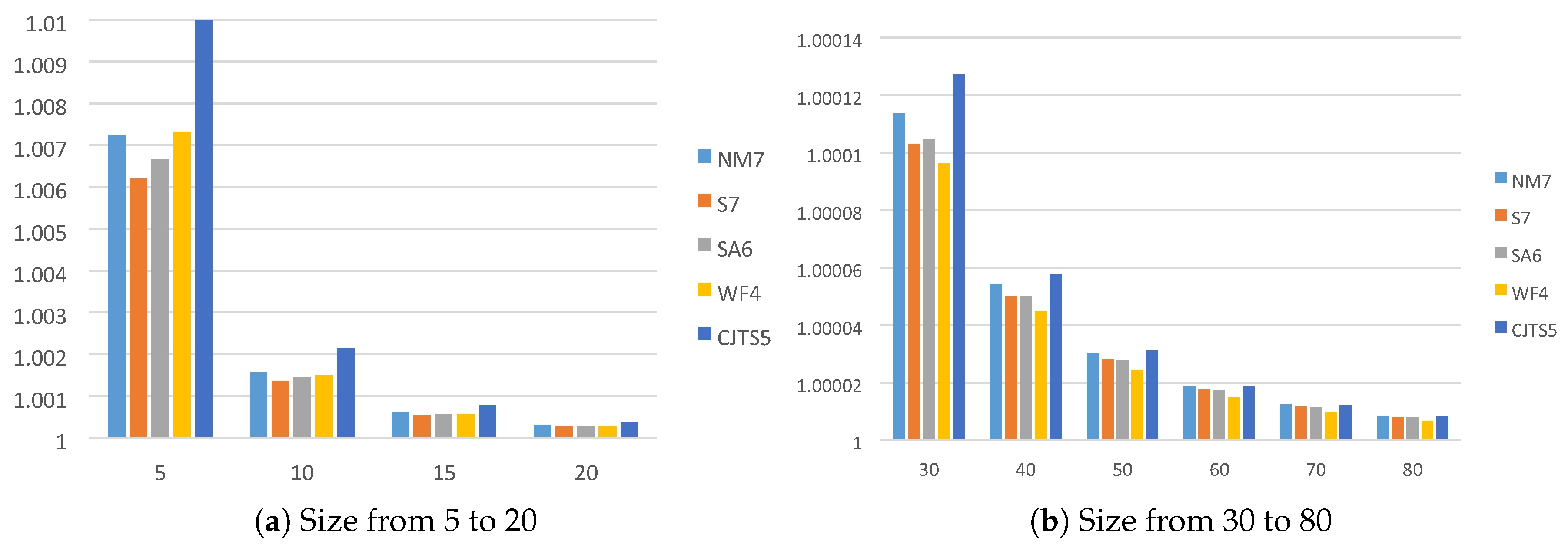
4. Efficiency Indices

As we have mentioned in the Introduction, we use indices $EI=p^{1/d}$ and $CEI$ to compare the different iterative methods.

To evaluate function F, n scalar functions are calculated and $n(n-1)$ for the first order divided difference $[·,·;F]$. In addition, to calculate an inverse linear operator, an $n\times n$ linear system must be solved; then, we have to do ${\displaystyle \frac{1}{3}}{n}^3+n^2-{\displaystyle \frac{1}{3}}n$ quotients/products for getting $LU$ decomposition and solving the corresponding triangular linear systems. Moreover, for solving m linear systems with the same matrix of coefficients, we need to do ${\displaystyle \frac{1}{3}}{n}^3+m{n}^2-{\displaystyle \frac{1}{3}}n$ products-quotients. In addition, we need $n^2$ products for each matrix-vector multiplication and $n^2$ quotients for evaluating a divided difference operator.

According to the last considerations, we calculate the efficiency indices $EI$ of methods CJST5, NM7, S7, SA6 and WF4. In case CJST5, for each iteration, we evaluate F three times and once $[·,·;F]$, so $n^2+2n$ functional evaluations are needed. Therefore, $E{I}_{CJST5}=5^{\frac{1}{n^2+2n}}$. The indices obtained for the mentioned methods are also calculated and shown in

Table 1. Efficiency indices for different methods.

Method	Order	NFE	$\mathit{EI}$
NM7	7	$2n^2+n$	$7^{\frac{1}{2n^2+n}}$
S7	7	$3n^2$	$7^{\frac{1}{3n^2}}$
SA6	6	$2n^2+n$	$6^{\frac{1}{2n^2+n}}$
WF4	4	$2n^2$	$4^{\frac{1}{2n^2}}$
CJST5	5	$n^2+2n$	$5^{\frac{1}{n^2+2n}}$

.

In

Table 2. Computational cost of the procedures.

Method	Order	$\mathit{NFE}$	$\mathit{NLS}1$	$\mathit{M}\times \mathit{V}$	$\mathit{CEI}$
NM7	7	$2n^2+3n$	4	3	$7^{\frac{1}{\frac{1}{3}{n}^3+11n^2+\frac{2}{3}n}}$
S7	7	$3n^2$	6	3	$7^{\frac{1}{\frac{1}{3}{n}^3+14n^2-\frac{1}{3}n}}$
SA6	6	$2n^2+n$	4	2	$6^{\frac{1}{\frac{1}{3}{n}^3+11n^2+\frac{2}{3}n}}$
WF4	4	$2n^2$	3	1	$4^{\frac{1}{\frac{1}{3}{n}^3+8n^2-\frac{1}{3}n}}$
CJST5	5	$n^2+2n$	3	0	$5^{\frac{1}{\frac{1}{3}{n}^3+5n^2+\frac{5}{3}n}}$

, we present the indices $CEI$ of schemes NM7, SA6, S7, WF4 and CJST5. In it, the amount of functional evaluations is denoted by $NFE$, the number of linear systems with the same $[·,·;F]$ as the matrix of coefficients is $NLS1$ and $M\times V$ represents the quantity of products matrix-vector. Then, in case CJST5, for each iteration, $n^2+2n$ functional evaluations are needed, since we evaluate three times the function F and one divided difference of first order $[a^{(k)},b^{(k)},F]$. In addition, we must solve three linear systems with $[a^{(k)},b^{(k)},F]$ as coefficients matrix (that is ${\displaystyle \frac{1}{3}}{n}^3+3n^2-{\displaystyle \frac{1}{3}}n$). Thus, the value of $CEI$ for CJST5 is

$$CE{I}_{CJST5}=5^{\frac{1}{\frac{1}{3}{n}^3+5n^2+\frac{5}{3}n}}.$$

Analogously, we obtain the indices $CEI$ of the other methods. In Figure 1, we observe the computational efficiency index of the different methods of size 5 to 80. The best index corresponds to our proposed scheme.

5. Numerical Examples

We begin this section checking the performance of the new method on the resulting system obtained by the discretization of Fisher’s partial differential equation. Thereafter, we compare its behavior with that of other known methods on some academic problems. For the computations, we have used $Matlab$ R2015a ( Natick, Massachusetts, USA) with variable precision arithmetic, with 1000 digits of mantissa. The characteristics of the computer are, regarding the processor, Intel(R) Core(TM) i7-7700 CPU @ 3.6 GHz, 3.601 Mhz, four processors and RAM 16 GB.

We use the estimation of the theoretical order of convergence p, called Computational Order of Convergence (COC), introduced by Jay [14] with the following expression:

$$p\approx COC=\frac{ln\left(\parallel F(x^{(k+1)}){\parallel }_2/{\parallel F(x^{(k)})\parallel }_2\right)}{ln(\parallel F(x^{(k)}){\parallel }_2/\parallel F(x^{(k-1)}){\parallel }_2)},k=1,2,\dots$$

and the Approximated Computational Order of Convergence (ACOC), defined by Cordero and Torregrosa in [15]

$$p\approx ACOC=\frac{ln(\parallel x^{(k+1)}-x^{(k)}{\parallel }_2/\parallel x^{(k)}-x^{(k-1)}{\parallel }_2)}{ln(\parallel x^{(k)}-x^{(k-1)}{\parallel }_2/\parallel x^{(k-1)}-x^{(k-2)}{\parallel }_2)}.$$

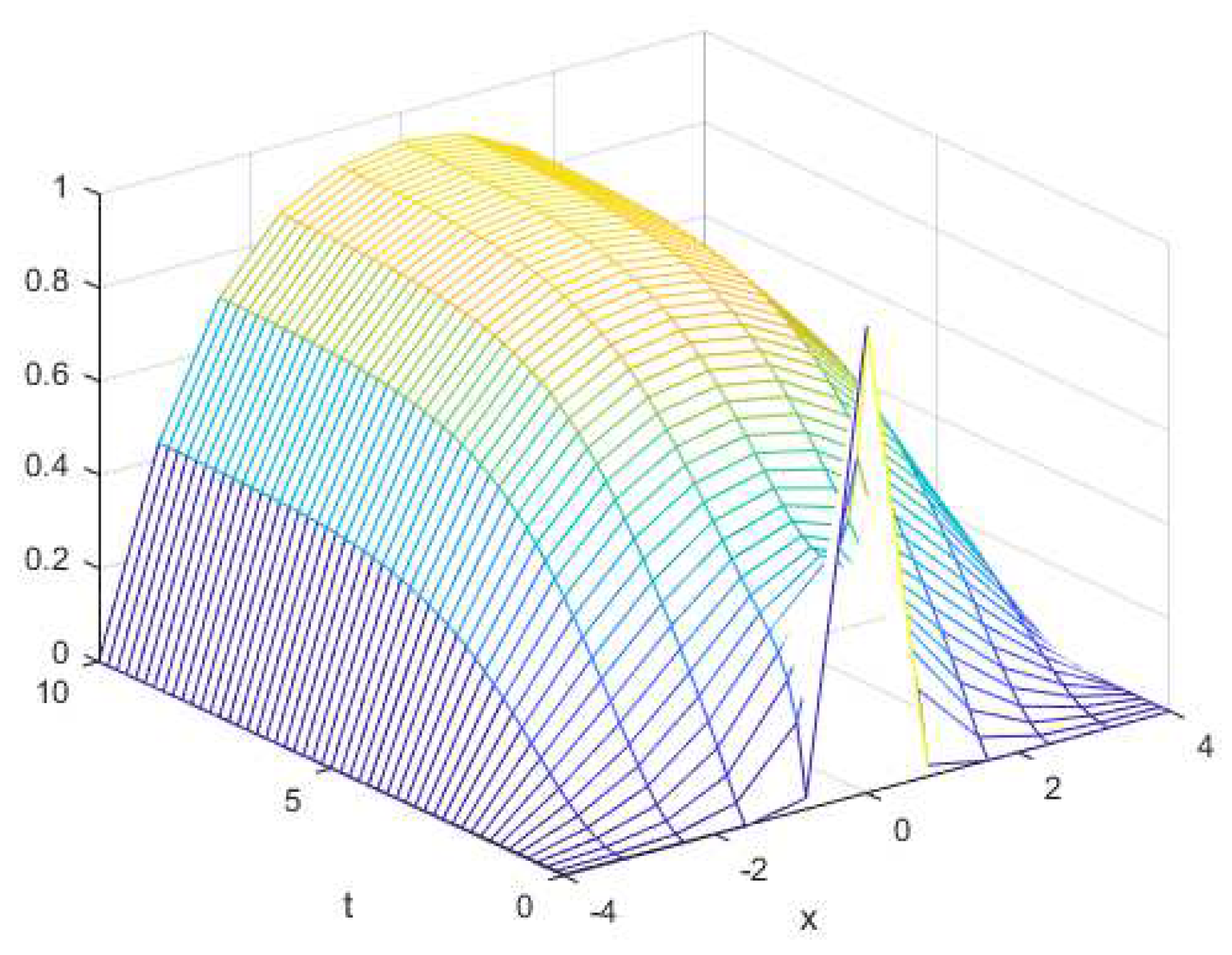
Example 1.

Fisher’s equation,

$$u_t=D{u}_{xx}+ru\left(1-\frac{u}{p}\right),x\in [a,b]t\ge 0,$$

(12)

was proposed in [16] by Fisher to model the diffusion process in population dynamics. In it, $D>0$ is the diffusion constant, r is the level of growth of the species and p is the carrying capacity. Lately, this formulation has proven to be fruitful for many other problems as wave genetics, economy or propagation.

Now, we study a particular case of this equation, when $r=p=1$ and the spatial interval is $[0,1]$, $u(x,0)=sec{h}^2(\pi x)$ and null boundary conditions.

We transform Example 1 in a set of nonlinear systems by applying an implicit method of finite differences, providing the estimated solution in the instant $t_k$ from the estimated one in $t_{k-1}$. The spacial step $h=1/n_x$ is selected and the temporal step is $k=T_{max}/n_t$, $n_x$ and $n_t$ being the quantity of subintervals in x and t, respectively, and $T_{max}$ is the final instant. Therefore, a grid of domain $[0,1]\times [0,T_{max}]$ with points $(x_i,t_j)$, is selected:

$$x_i=0+ih,i=0,1,\dots ,n_x,t_j=0+jk,j=0,1,\dots ,n_t.$$

Our purpose is to estimate the solution of problem (12) at these points, by solving many nonlinear systems, as much as the number of temporal nodes $t_j$. For it, we use the following finite differences of order $\mathcal{O}(k+h^2)$:

$$\begin{array}{cc}\hfill u_t(x,t)& \approx {\displaystyle \frac{u(x,t)-u(x,t-k)}{k}},\hfill \\ \hfill u_{xx}(x,t)& \approx {\displaystyle \frac{u(x+h,t)-2u(x,t)+u(x-h,t)}{h^2}}.\hfill \end{array}$$

By denoting the approximation of the solution at $(x_i,t_j)$ as $u_{i,j}$, and, by replacing it in Example 1, we get the system

$$k{u}_{i+1,j}+(k{h}^2-2k-h^2)u_{i,j}-k{h}^2{u}_{i,j}^2+k{u}_{i-1,j}=-h^2{u}_{i,j-1},$$

for $i=1,2,\dots ,n_x-1$ and $j=1,2,\dots ,n_t$. The unknowns of this system are $u_{1,j},u_{2,j},\dots ,u_{n_x-1,j},$ that is, the approximations of the solution in each spatial node for the fixed instant $t_j$. Let us remark that, for solving this system, the knowledge of solution in $t_{j-1}$ is required.

Let us observe (

Table 3. Fisher results by CJST5 and different $T_{max}$.

${\mathit{T}}_{\mathit{max}}$	${\mathit{n}}_{\mathit{x}}$	${\mathit{n}}_{\mathit{t}}$	$\parallel \mathit{F}({\mathit{x}}^1)\parallel$	$\parallel \mathit{F}({\mathit{x}}^2)\parallel$	$\parallel \mathit{F}({\mathit{x}}^3)\parallel$	COC
$0.1$	10	20	8.033 $\times {10}^{-9}$	2.356 $\times {10}^{-35}$	3.243 $\times {10}^{-68}$	1.2385
$0.1$	10	200	8.679 $\times {10}^{-13}$	3.203 $\times {10}^{-44}$	7.623 $\times {10}^{-77}$	1.0379
1	10	20	4.158 $\times {10}^{-5}$	3.4 $\times {10}^{-25}$	1.679 $\times {10}^{-56}$	1.5585
1	10	200	8.033 $\times {10}^{-9}$	2.356 $\times {10}^{-35}$	3.243 $\times {10}^{-68}$	1.2385
10	10	20	nc
10	10	50	0.01945	2.757 $\times {10}^{-11}$	1.953 $\times {10}^{-38}$	3.0683

) that the results improve when the temporal step is smaller. In this case, the COC is not a good estimation of the theoretical error. In Figure 2, we show the approximated solution of the problem when $T_{max}=10$, by taking $n_t=50$, $n_x=10$ and using method CJST5.

In the rest of examples, we are going to compare the performance of the proposed method with the schemes presented in the Introduction as well as with the Newton-type method replacing the Jacobian matrix by the divided difference operator, that is, the Samanskii’s scheme (see [6]).

Example 2.

Let us define the nonlinear system

$$\left\{\begin{array}{c}cos(x_2)-sin(x_1)=0,\hfill \\ x_3^{x_1}-1/x_2=0,\hfill \\ e^{x_1}-x_3^2=0.\hfill \end{array}\right.$$

We use, in this example, the starting estimation $x^{(0)}={(1.25,1.25,1.25)}^T$, the solution being $\overline{x}\approx {(0.9096,0.6612,1.576)}^T$.

Table 4. Numerical results for Example 2.

	Samanskii	CJST5	WF4	SA6	S7	NM7
$\parallel x^{(1)}-x^{(0)}\parallel$	1.415	0.8848	0.8539	0.8934	0.9148	0.9355
$\parallel x^{(2)}-x^{(1)}\parallel$	0.5427	0.247	0.2039	0.2689	0.2942	0.3098
$\parallel x^{(3)}-x^{(2)}\parallel$	0.1738	0.01159	0.006249	0.005301	0.01069	0.02667
ACOC	1.1875	2.3976	2.433	3.2705	2.9221	4.25
$\parallel F(x^{(1)})\parallel$	0.1954	0.1282	0.1038	0.1385	0.1817	0.2098
$\parallel F(x^{(2)})\parallel$	0.02369	0.009956	0.004815	0.003584	0.006462	0.01669
$\parallel F(x^{(3)})\parallel$	0.00269	2.805 $\times {10}^{-8}$	7.663 $\times {10}^{-8}$	4.009 $\times {10}^{-11}$	8.074 $\times {10}^{-12}$	1.333 $\times {10}^{-9}$
COC	1.0313	5.0015	3.5983	5.0104	6.1445	6.4561

shows the residuals $\parallel x^{(k)}-x^{(k-1)}\parallel$ and $\parallel F(x^{(k)})\parallel$ for $k=1,2,3$ as well as ACOC and COC. We observe that the COC index is better than the corresponding ACOC of the other methods. In addition, the value $\parallel x^3-x^2\parallel$ is better or similar to that of S7 and NM7 methods, both of them of order 7.

Example 3.

We consider now

$$\sum _{j=1}^n{x}_j-x_i-e^{-x_i}{x}_i=0,i=1,2,\dots ,n.$$

The numerical results are displayed in

Table 5. Numerical results for Example 3.

	Samanskii	CJST5	WF4	SA6	S7	NM7
$\parallel x^{(1)}-x^{(0)}\parallel$	1.036	0.8249	0.9116	0.8499	0.7847	0.7897
$\parallel x^{(2)}-x^{(1)}\parallel$	0.2552	0.03432	0.121	0.05932	0.00583	0.0008995
$\parallel x^{(3)}-x^{(2)}\parallel$	0,009667	1.487 $\times {10}^{-11}$	9.264 $\times {10}^{-6}$	5.367 $\times {10}^{-10}$	2.529 $\times {10}^{-21}$	1.048 $\times {10}^{-28}$
ACOC	2.3361	6.7807	4.6937	6.9572	8.6247	4.25
$\parallel F(x^{(1)})\parallel$	1.944	0.2742	0.9634	0.4735	0.04665	0.007196
$\parallel F(x^{(2)})\parallel$	0.0773	1.19 $\times {10}^{-10}$	7.411 $\times {10}^{-5}$	4.293 $\times {10}^{-9}$	2.023 $\times {10}^{-20}$	8.381 $\times {10}^{-28}$
$\parallel F(x^{(3)})\parallel$	2.65 $\times {10}^{-5}$	2.839 $\times {10}^{-59}$	9.644 $\times {10}^{-22}$	1.3 $\times {10}^{-57}$	9.093 $\times {10}^{-149}$	2.621 $\times {10}^{-202}$
COC	2.4743	5.1932	4.1045	6.0328	6.9895	6.9987

. The initial estimation is $x^{(0)}={(0.25,0.25,\dots ,0.25)}^T$ and the size of the system is $n=10$, the solution being $\overline{x}={(0,0,\dots ,0)}^T$. We show the same information as in the previous example.

Example 4.

The third example is given by the system:

$$x_i+1-2log\left(1+\sum _{j=1}^n{x}_j-x_i\right)=0,i=1,2,\dots ,n.$$

Its solution is $\overline{x}\approx {(9.376,9.376,\dots ,9.376)}^T$. By using the starting guess $x^{(0)}={(1,1,\dots ,1)}^T$ with $n=10$, we obtain the results appearing in

Table 6. Numerical results for Example 4.

	Samanskii	CJST5	WF4	SA6	S7	NM7
$\parallel x^{(1)}-x^{(0)}\parallel$	6.013	40.68	67.88	73.31	34.3	39.23
$\parallel x^{(2)}-x^{(1)}\parallel$	12.15	13.83	36.07	56.74	17.15	7.369
$\parallel x^{(3)}-x^{(2)}\parallel$	10.11	0.0002872	0.06643	0.02688	0.0001485	5.422 $\times {10}^{-8}$
ACOC	-	9.9941	9.9587	29.874	16.819	4.25
$\parallel F(x^{(1)})\parallel$	10.84	11.03	30.43	48.74	13.42	5.842
$\parallel F(x^{(2)})\parallel$	6.084	0.0002263	0.05234	0.02117	0.000117	4.272 $\times {10}^{-8}$
$\parallel F(x^{(3)})\parallel$	1.162	9.286 $\times {10}^{-28}$	6.508 $\times {10}^{-12}$	1.807 $\times {10}^{-20}$	3.105 $\times {10}^{-40}$	7.552 $\times {10}^{-65}$
COC	2.8651	4.9888	3.583	5.3744	7.0313	6.9755

.

The different methods give us the expected results, according to their order of convergence.

Example 5.

Finally, the last example that we consider is:

$$arctan(x_i)+1-2\left(\sum _{j=1}^n{x}_j^2-x_i^2\right)=0.$$

The solution of it is $\overline{x}\approx {(0.1758,0.1758,\dots ,0.1758)}^T$. By using the initial estimation $x^{(0)}={(0.5,0.5,\dots ,0.5)}^T$ with $n=20$, we obtain the numerical results displayed in

Table 7. Numerical results for Example 5.

	Samanskii	CJST5	WF4	SA6	S7	NM7
$\parallel x^{(1)}-x^{(0)}\parallel$	0.9503	1.323	1.272	1.368	1.394	1.393
$\parallel x^{(2)}-x^{(1)}\parallel$	0.3912	0.1266	0.177	0.0821	0.05639	0.05732
$\parallel x^{(3)}-x^{(2)}\parallel$	0.1013	4.988 $\times {10}^{-5}$	0.0007407	6.903 $\times {10}^{-7}$	7.214 $\times {10}^{-9}$	6.655 $\times {10}^{-9}$
ACOC	1.5229	3.3404	2.776	4.1543	4.9485	4.25
$\parallel F(x^{(1)})\parallel$	8.324	1.706	2.471	1.075	0.7257	0.7381
$\parallel F(x^{(2)})\parallel$	1.445	0.0006179	0.009181	8.552 $\times {10}^{-6}$	8.937 $\times {10}^{-8}$	8.245 $\times {10}^{-8}$
$\parallel F(x^{(3)})\parallel$	0.0902	1.206 $\times {10}^{-20}$	5.635 $\times {10}^{-12}$	5.437 $\times {10}^{-36}$	8.115 $\times {10}^{-56}$	3.521 $\times {10}^{-56}$
COC	1.5839	4.8559	3.791	5.9219	6.953	6.9577

.

It is observed in Table 5, Table 6 and Table 7 that, for the proposed academic problems, the introduced method (CJST5) shows a good performance comparable with higher-order methods. Of course, the worst results are those obtained by Samanskii’s method, but it has been included because it is the Jacobian-free version of Newton’s scheme and it is also the first step of our proposed scheme. Let us also remark that, when only three iterations are calculated, the index COC gives more reliable information than the ACOC one in all of the examples.

6. Conclusions

In this paper, we design a family of iterative methods for solving nonlinear systems with fourth-order convergence. This family does not use Jacobian matrices and one of its elements has order five. The relationship between the proposed method and other known ones in terms of efficiency index and computational efficiency index allows us to see that our method is more efficient than the other ones. In addition, its error bounds are smaller with the same number of iterations in some cases. Thus, our proposal is competitive mostly for big size systems.