2. Preliminaries and Definitions
Let denote n-dimensional Euclidean space and be its non-negative orthant. Let and be closed convex cones in and , respectively, with nonempty interiors. For a real-valued twice differentiable function defined on an open set in , denote by the gradient vector of g with respect to x at and the Hessian matrix with respect to x at . Similarly, , , and are also defined.
Let be an open set. Let be a differentiable function and where is the range of f such that G is strictly increasing on the range of f, and
Definition 1. Let E be a compact convex set in . The support function of E is defined by: A support function, being convex and everywhere finite, has a subdifferential, that is there exists a such that: The subdifferential of is given by: For a convex set , the normal cone to F at a point is defined by: When E is a compact convex set, if and only if or, equivalently,
Definition 2. The positive polar cone of a cone is defined by: Now, we give the definitions of -invex/-pseudoinvex and -bonvex/-pseudobonvex functions with respect to η.
Definition 3. If there exist functions and s.t. then f is called -invex at with respect to Definition 4. If there exists functions and such that then f is called -pseudoinvex at with respect to Definition 5. is -bonvex at if there exist and if ,
: Definition 6. is -pseudobonvex at if there exist and a function if
: Remark 1. If , then Definitions 5 and 6 become the -bonvex/-pseudobonvex functions with the same η.
Now, we present here functions that are -bonvexity/-pseudobonvexity, but neither -bonvex/-pseudobonvex nor -invex/-pseudoinvex with the same .
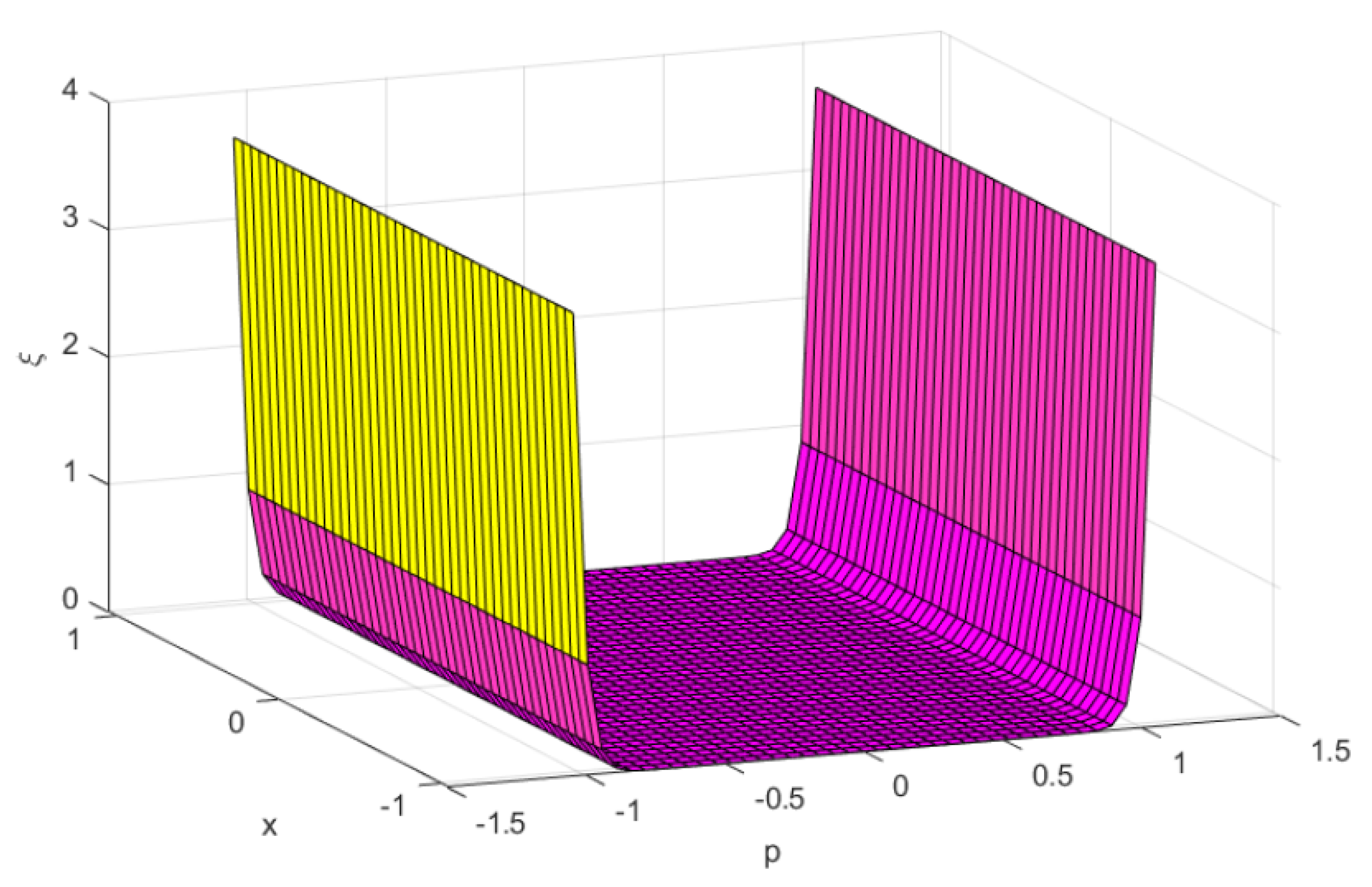
Example 1. Let be defined as A function is defined as: Let be given as: Furthermore, is given by: To demonstrate that f is -bonvex at , we need to demonstrate that
Putting the estimations of , and G in the above articulation, we get: for which at , we get: (clearly, from Figure 1).
Therefore, f is -bonvex at .
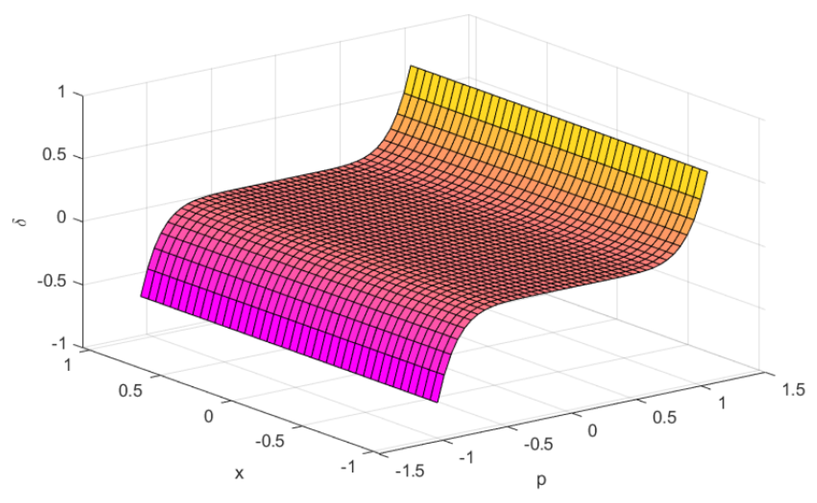
for which at the above equation may not be nonnegative (see Figure 2).
Therefore, f is not -bonvex at with the same η.
Specifically, at point and at , we find that: This shows that f is not -invex with the same η.
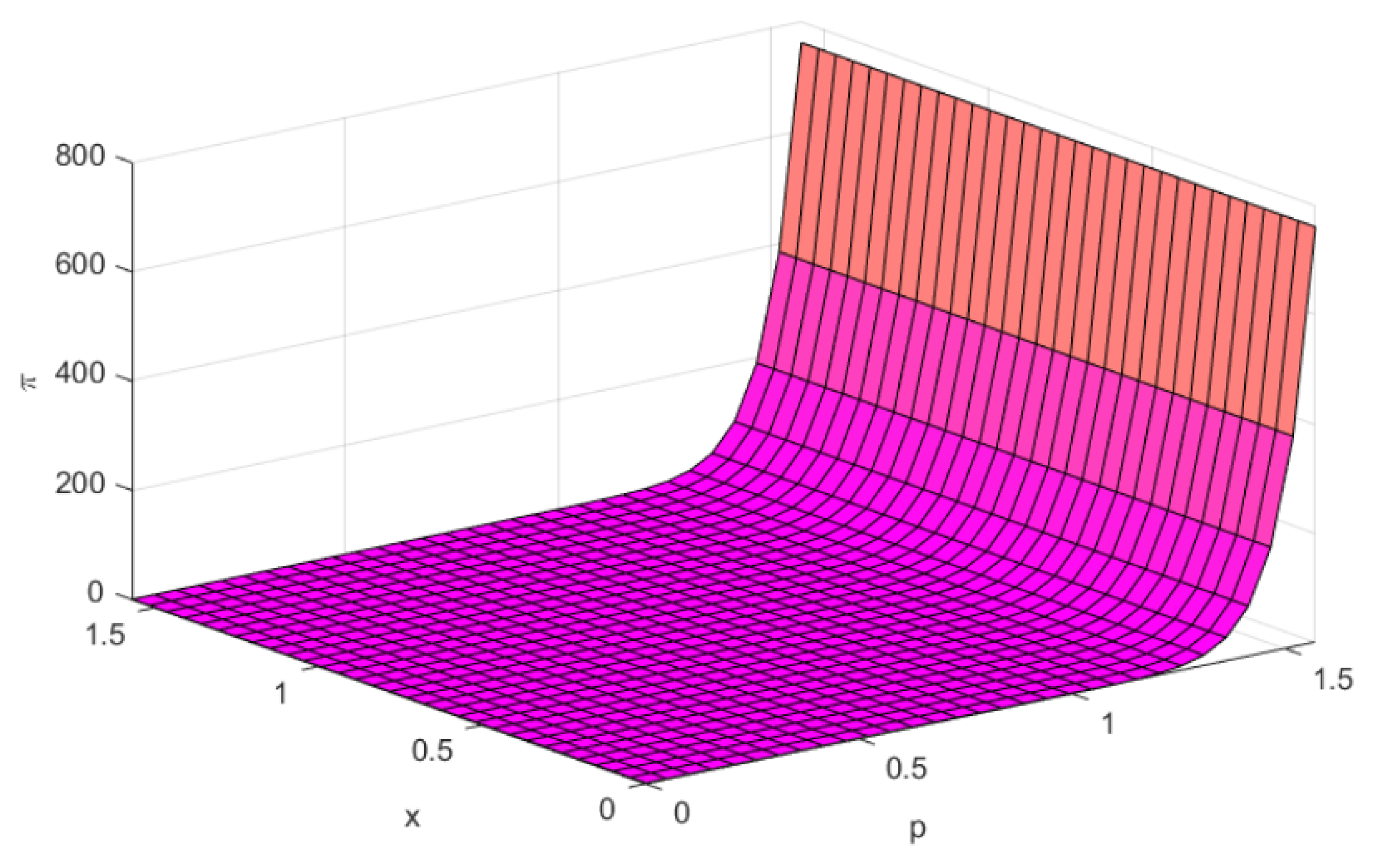
Example 2. Let be defined as: A function is defined as: Let be given as: Furthermore, is given by: Now, we have to claim that f is -bonvex at . For this, we have to prove that
Substituting the values of , and G in the above expression, we obtain: Clearly, from Figure 3, and Therefore, f is -bonvex at with respect to
This implies that f is not -bonvex at with the same η.
At the point , we find that: Hence, f is not -invex at with the same η.
Example 3. Let be defined as: A function is defined as: Let be given as: Furthermore, is given by: Presently, we need to demonstrate that f is -pseudobonvex at concerning η. For this, we have to show that: Putting the estimations of , and G in the above articulation, we get: for which at , we obtain
Next,
Substituting the estimations of , and G in the above articulation, for which at , we obtain Therefore, f is -pseudobonvex at .
Substituting the values of , and G in the above expression, we obtain: for which at , we find that
Substituting the values of , and G in the above expression, we obtain: for which at , we get Therefore, f is not -pseudobonvex at .
Similarly, at , we find that Next, In the same way, at , we find that, Hence, f is not -pseudoinvex at with the same η.
3. Non-Differentiable Second-Order Symmetric Primal-Dual Pair over Arbitrary Cones
” In this section, we formulate the following pair of second-order non-differentiable symmetric dual programs over arbitrary cones:
(NSOP) Minimize
subject to
:
(NSOD) Maximize
subject to
where
and
are positive polar cones of
and
, respectively. Let
and
be feasible solutions of (NSOP) and (NSOD), respectively.
Theorem 1 (Weak duality theorem)
. Let and . Let:
- (i)
and be -bonvex and -invex at v, respectively, with the same η,
- (ii)
and be -boncave and -incave at z, respectively, with the same ξ,
- (iii)
- (iv)
Proof. From Hypothesis
and the dual constraint (
5), we obtain
The above inequality follows
:
which upon using (
6) and (
7) yields
Again, from Hypothesis , we obtain
:
and:
Combining the above inequalities, we get
:
Using Inequality (
10), it follows that
:
Similarly, using , and primal constraints, it follows that
:
Adding Inequalities (
11) and (
12), we get
:
Finally, using the inequalities and we have
:
Since , we obtain
:
Hence, the result. □
A non-trivial numerical example for legitimization of the weak duality theorem.
Example 4. Let be a function given by: Suppose that and
Further, let be given by: Furthermore, and
Putting these values in (NSOP) and (NSOD), we get:
(ENSOP) Minimize T() =
(ENSOD)Maximize W()
Firstly, we will try to prove that all the hypotheses of the weak duality theorem are satisfied:
is -bonvex at ,
at
Obviously, is -invex at .
is -boncave at and we obtain
at
Naturally, is -invex at .
Obviously, and
Hence, all the assumptions of Theorem 1 hold.
Verification of the weak duality theorem: Let and . To validate the result of the weak duality theorem, we have to show that
Substituting the values in the above expression, we obtain:
At the feasible point, the above expression reduces:
Hence, the weak duality theorem is verified.
Remark 2. Since every bonvex function is pseudobonvex, therefore the above weak duality theorem for the symmetric dual pair (NSOP) and (NSOD) can also be obtained under -pseudobonvex assumptions.
Theorem 2 (Weak duality theorem)
. Let and . Let:
- (i)
be -pseudobonvex and be -pseudoinvex at v with the same η,
- (ii)
be -pseudoboncave and be -pseudoinvex at z with the same ξ,
- (iii)
- (iv)
Proof. The proof follows on the lines of Theorem 1. □
Theorem 3 (Strong duality theorem)
. Let be an optimum of problem (NSOP). Let:
is positive or negative definite,
.
Then, , and there exists such that is an optimum for the problem (NSOD).
Proof. Since
is an efficient solution of (NSOD), therefore by the conditions in [
15], such that
:
:
:
:
:
:
Premultiplying Equation (
15) by
and using (
16)–(
18), we get
Using Hypothesis
, we get:
From Equation (
15) and Hypothesis
we obtain:
Now, suppose
. Then, Equation (
14) and Hypothesis
yield
which along with Equations (
24) and (
25) gives
Thus,
, a contradiction to Equation (
22). Hence, from (
23):
Using Equations (
16)–(
18), we have
:
and now, Equation (
24) gives
:
which along with Hypothesis
yields:
Furthermore, it follows from Equations (
14), (
24), and (
29) and Hypotheses
that:
Therefore, Equation (
30) gives:
Moreover, Equation (
13) together with (
24) and using
yields
:
Let
Then,
as
is a closed convex cone. Upon substituting
in place of
y in (
33), we get
:
which in turn implies that for all
we obtain
:
Furthermore, by letting
and
, simultaneously in (
33), this yields
:
Using Inequality (
31), we get:
Thus, satisfies the dual constraints.
Now, using Equations (
30) and (
31), we obtain:
Furthermore,
then we obtain
. Furthermore,
D is a compact convex set.
Thus, after using (
20), (
29), (
38) and (
39), we get that the values of the objective functions of (NSOP) and (NSOD) at
and
are the same. By using duality Theorems 1 and 2, it is easily shown that
is an optimal solution of (NSOD). □
Theorem 4 (Strict converse duality theorem) Let be an optimum of problem (NSOD). Let:
is positive or negative definite,
.
Then, , and there exists such that is an optimum for the problem (NSOP).
Proof. The proof follows on the lines of Theorem 3. □


