Understanding the Evolution of Tree Size Diversity within the Multivariate Nonsymmetrical Diffusion Process and Information Measures

Abstract

This study focuses on the stochastic differential calculus of Itô, as an effective tool for the analysis of noise in forest growth and yield modeling. Idea of modeling state (tree size) variable in terms of univariate stochastic differential equation is exposed to a multivariate stochastic differential equation. The new developed multivariate probability density function and its marginal univariate, bivariate and trivariate distributions, and conditional univariate, bivariate and trivariate probability density functions can be applied for the modeling of tree size variables and various stand attributes such as the mean diameter, height, crown base height, crown width, volume, basal area, slenderness ratio, increments, and much more. This study introduces generalized multivariate interaction information measures based on the differential entropy to capture multivariate dependencies between state variables. The present study experimentally confirms the effectiveness of using multivariate interaction information measures to reconstruct multivariate relationships of state variables using measurements obtained from a real-world data set.

1. Introduction

Stand attributes prediction has been a popular and challenging research topic in both forestry science and economics due to its importance to forest managers, governments, as well as economic stakeholders in recent years. Sustainable forest management process requires growth and yield models that enable prediction of the development of forest stands under different natural environment, economic and sociocultural pillars. Diameter at the breast height, total tree height, crown base height and crown width size dimensions (in the sequel—tree size variables), and the number of trees per hectare are substantial components of stand growth and yield models whose evolution provide details on stand development [1]. These tree size variables are the most important predictor variables for the estimation of stem volume, biomass and carbon storage in natural forests. Rational management needs the dynamical individual tree growth and yield models because they provide the evolution for forward and backward directions, and produce detailed information about changes of stand structure [2]. Tree size variables can be modeled as a complex system, each with its own regulatory mechanism and all continuously interacting between them. The mathematical and numerical methods used to describe the dynamic of biological system are largely concerned with the derivation, and use of ordinary stochastic and partial differential equations [3,4]. Individual-tree and stand-level growth models traditionally are represented by a system of ordinary differential equations [5]. The basic idea is to describe a system of ordinary differential equations, which specifies changes of a suitable number of tree or stand size variables via age (time) and to summarize the relevant information about the size variables’ dependence. One of the advantages of ordinary differential equation approach lies in parameter interpretation, which simplifies the results’ interpretation by using asymptotic and inflection points. Unfortunately, an ordinary differential equations approach has some limitations, including the absence of the factor of tree size variables dependence and the variance-covariance matrix of tree size variables [6,7,8]. In addition, eco-regional growth and yield models must be updated by including the random factor of a stand quality [9]. Statistical analysis of developed relationships between tree size components at a given stand or location is usually performed based on statistical indexes and tests for an observed dataset. However, no single equation for tree size variables has gained global acceptance. The traditional method is to try a variety of models and choose the best fitted equation based on a particular mathematical norm, such as the least square error or a likelihood norm. The disadvantages of this method of choosing are that it is laborious because too many equations need to be tried and empirical choices of candidate equations make the results subjective. In order to overcome these disadvantages, the multivariate stochastic differential equations have recently gained a lot of attention. Stochastic differential equations are often used in the modeling of population dynamic [10,11,12], tumor growth [13], chemical reaction networks [14], environmental pollution [15,16], forest growth and yield [17]. The deterministic differential equation carries its solution, which is completely determined in the value sense by knowledge of boundary and initial conditions. It means that the identical initial and boundary conditions generate identical solutions. Conversely, a stochastic differential equation (SDE) is a differential equation with a solution which is a stochastic process. Because tree diameter at breast height, total tree height, crown base height and crown width are empirically correlated, the multivariate SDE models should be considered [6,8,18].

The greatest advantage of multivariate SDE approach is that it provides sufficient flexibility to fit a large variety of nested models for a separate tree size and stand size variable, which facilitates the selection and comparison of newly developed models by using information measures technique [19,20,21]. In order to construct the multi-information measures, it is necessary to obtain the probability density function of tree size variable, which in this study are obtained from a 4-variate Bertalanffy SDE describing the development of the tree size variables against the age. SDEs models are much more flexible than deterministic models, but come at a computational cost. The problem of representing the mechanisms governing the evolution of univariate tree size distribution have been directed using univariate SDEs in fluid mechanics [22,23]. Central research finding in tree size distributions by Kohyama et al. [24] is the fact that they are positively skewed. Theoretical studies of tree size growth confirmed that the size frequency distribution of trees is inverse J-shaped, with many small trees and few larger trees due asymmetric competition [25]. The Vasicek type 4-variate fixed effects SDE presented by Rupšys and Petrauskas [6] defines changes in stem diameter and height distribution with age of a stand, which takes into account the 4-variate normal distribution at a given stand age, t. This study focuses on the alternative nonsymetric Bertalanfy type 4-variate diffusion process which links between tree diameter, height, crown base height and crown width dynamics, and their 4-variate lognormal probability density function development. Traditionally stochastic tree growth processes are observed in multiple populations (stands), so to quantify of both between and within stand variation the framework of the random effect parameters have been studied [6,11,26,27,28]. In this basis, the introduction of only one additional random effect parameter allows capturing arbitrary wide stand dependencies without increasing model order, hence retaining model simplicity and ease of parameters estimation. The fixed and mixed parameters estimation for discretely observed SDE is a complex problem and during the past decades it has attracted the attention a lot of researchers. Taking the applicability and generality into account, maximum-likelihood estimation is in the lead among others [29,30]. Generally, when both system noise and random effects are considered, the exact form of the maximum likelihood function is unavailable, and then an approximated maximum likelihood procedure is used [31].

This study focuses on a mixed-effects parameters 4-variate Bertalanffy type diffusion process satisfying an Itô [32] SDE conditional on an initial value taken at a fixed initial time (age) point. In an even-aged stand tree size components’ distribution shows some asymmetry. The goal of this paper is to present a unified perspective of the tree growth in a forest stand network as a nonsymetric Markov process in a multidimensional vector space. Another goal is to study in a general way the main methods of cross comparisons of all new developed growth models by using the Shannon type differential entropy. In the Results and Discussion, we consider possible application to the study of information sharing amongst tree size variables using a dataset of the diameter at breast height, tree height, crown base height and crown width measurements in Scots pine (Pinus Sylvestris L.) stands in Lithuania. All results are implemented in symbolic algebra system MAPLE.

2. Materials and Methods

This paper focuses on a 4-variate Bertalanffy type SDE to study the tree size variables (diameter at breast height, D(t), tree height, H(t), crown base height, CH, and crown width, CW) distribution problem in forest stands. This results in an exact 4-variate asymmetrical conditional (transition) probability density function, whose parameters can be estimated by maximum likelihood procedure based on discrete time observations. The random effects are included to describe between-stand variability. Proceeding as we have in the bivariate Bertalanffy type SDE model [8] that describes the development of the tree size variables evolving in M different stands, the mixed effect parameters 4-variate Bertalanffy type SDE model in a general manner are defined by:

$$d{X}^i(t)=A\left(X^i(t)\right)dt+Q{\left(X^i(t)\right)}^{\frac{1}{2}}·dW(t),i=1,2,\dots ,\mathrm{M}$$

(1)

here: M is the total number of stands used for model fitting, t is the time (stand age), $X(t)={\left(X_1(t),X_2(t),X_3(t),X_4(t)\right)}^T={\left(D(t),H(t),CH(t),CW(t)\right)}^T$, $t\in \left[t_0;T\right]$, $t_0\ge 0$, $X(t_0)=x_0={\left(x_{10},x_{20},x_{30},x_{40})\right)}^T$, $x_{s0}\ge 0$, $1\le s\le 4$, the drift vector Aⁱ (x) is defined as:

$$A^i(x)={\left(\frac{\left({\alpha }_1+{\phi }_1^i\right){\beta }_1{\gamma }_1}{e^{{\beta }_1\left(t-t_0\right)}-{\gamma }_1}{x}_1,\frac{\left({\alpha }_2+{\phi }_2^i\right){\beta }_2{\gamma }_2}{e^{{\beta }_2\left(t-t_0\right)}-{\gamma }_2}{x}_2,\frac{\left({\alpha }_3+{\phi }_3^i\right){\beta }_3{\gamma }_3}{e^{{\beta }_3\left(t-t_0\right)}-{\gamma }_3}{x}_3,\frac{\left({\alpha }_4+{\phi }_4^i\right){\beta }_4{\gamma }_4}{e^{{\beta }_4\left(t-t_0\right)}-{\gamma }_4}{x}_4\right)}^T$$

(2)

the diffusion matrix $Q(x)$ is defined as:

$$Q(x)=\left(C(x)B^{\frac{1}{2}}\right){\left(C(x)B^{\frac{1}{2}}\right)}^T=C(x)BC(x)=\left(\begin{array}{cccc}{\sigma }_{11}{x}_1^2& {\sigma }_{12}{x}_1{x}_2& {\sigma }_{13}{x}_1{x}_3& {\sigma }_{14}{x}_1{x}_4\\ {\sigma }_{21}{x}_1{x}_2& {\sigma }_{22}{x}_2^2& {\sigma }_{23}{x}_2{x}_3& {\sigma }_{24}{x}_2{x}_4\\ {\sigma }_{31}{x}_1{x}_3& {\sigma }_{32}{x}_2{x}_3& {\sigma }_{33}{x}_3^2& {\sigma }_{31}{x}_3{x}_4\\ {\sigma }_{41}{x}_1{x}_4& {\sigma }_{42}{x}_2{x}_4& {\sigma }_{43}{x}_3{x}_4& {\sigma }_{44}{x}_4^2\end{array}\right)$$

(3)

$$B=\left(\begin{array}{cccc}{\sigma }_{11}& {\sigma }_{12}& {\sigma }_{13}& {\sigma }_{14}\\ {\sigma }_{12}& {\sigma }_{22}& {\sigma }_{23}& {\sigma }_{24}\\ {\sigma }_{13}& {\sigma }_{23}& {\sigma }_{33}& {\sigma }_{34}\\ {\sigma }_{14}& {\sigma }_{24}& {\sigma }_{34}& {\sigma }_{44}\end{array}\right),C(x)=\left(\begin{array}{cccc}{x}_1& 0& 0& 0\\ 0& x_2& 0& 0\\ 0& 0& x_3& 0\\ 0& 0& 0& x_4\end{array}\right)$$

$W^i(t)={\left(W_1^i(t),W_2^i(t),W_3^i(t),W_4^i(t)\right)}^T$, $t\in \left[t_0;T\right]$, i = 1, 2, …, M, are independent 4-variate Brownian motions, ${\phi }_s^i$, $1\le s\le 4$, i = 1, 2, …, M, are independent and normally distributed random variables with zero mean and constant variances (${\phi }_s^i~N\left(0;{\sigma }_s^2\right)$), $\left\{{\alpha }_1,{\alpha }_2,{\alpha }_3,{\alpha }_4,{\beta }_1,{\beta }_2,{\beta }_3,{\beta }_4,{\gamma }_1,{\gamma }_2,{\gamma }_3,{\gamma }_4,{\sigma }_{11},{\sigma }_{12},{\sigma }_{13},{\sigma }_{14},{\sigma }_{22},{\sigma }_{23},{\sigma }_{24},{\sigma }_{33},{\sigma }_{34},{\sigma }_{44},{\sigma }_1,{\sigma }_2,{\sigma }_3,{\sigma }_4\right\}$ are fixed effect parameters to be estimated which fulfill conditions: $t\ge t_0>\min \left\{\frac{\ln \left({\gamma }_1\right)}{{\beta }_1},\frac{\ln \left({\gamma }_2\right)}{{\beta }_2},\frac{\ln \left({\gamma }_3\right)}{{\beta }_3},\frac{\ln \left({\gamma }_4\right)}{{\beta }_4}\right\}$, ${\beta }_1,{\beta }_2,{\beta }_3,{\beta }_4>0$, ${\alpha }_1+{\phi }_1^i,{\alpha }_2+{\phi }_2^i,{\alpha }_3+{\phi }_3^i,{\alpha }_4+{\phi }_4^i\ge 1$, and $W^i(t)$, ${\phi }_s^i$, are mutually independent for all 1 ≤ i ≤ M, $1\le s\le 4$. The Bertalanffy type 4-variate SDE can be converted into a well-studied 4-variate Ornstein-Uhlenbeck (1930) [33] process by the transformation $Y(t)={\left(e^{{\beta }_{i}t}\ln X_i(t),i=1,\dots ,4\right)}^T$ and solved explicitly. The solution is a conditional random vector $\left(X^i(t)|X^i(t_0)=x_0\right)={\left(X_s^i(t)|X_s^i(t_0)=x_{s0},s=1,\dots ,4\right)}^T$ that has a 4-variate lognormal distribution $L{N}_4\left({\mu }^i(t);\mathsf{\Sigma }(t)\right)$, i = 1, 2, … M, with the mean vector ${\mu }^i(t)$:

$${\mu }^i(t)={\left({\mu }_s^i(t),1\le s\le 4\right)}^T={\left(\ln (x_{s0})+\left({\alpha }_s+{\phi }_s^i\right)\ln \left(\frac{1-{\gamma }_s\exp (-{\beta }_{s}t)}{1-{\gamma }_s\exp (-{\beta }_s{t}_0)}\right)-\frac{{\sigma }_{ss}}{2}\left(t-t_0\right),1\le s\le 4\right)}^T$$

(4)

the variance-covariance matrix $\mathsf{\Sigma }(t)$:

$$\mathsf{\Sigma }(t)={\left(v_{su}(t)\right)}_{s,u=1,\dots ,4}={\left({\sigma }_{su}\left(t-t_0\right)\right)}_{s,u=1,\dots ,4},{\sigma }_{su}={\sigma }_{us},v_{su}(t)=v_{us}(t)$$

(5)

and the probability density function:

$$f\left(x_1,x_2,x_3,x_4,t|{\theta }^f,{\phi }^i\right)=\frac{1}{{\left(2\pi \right)}^2{\left|\mathsf{\Sigma }(t)\right|}^{\frac{1}{2}}(x_1·x_2·x_3·x_4)}\exp \left(-\frac{1}{2}\mathsf{\Omega }(x_1,x_2,x_3,x_4,t)\right)$$

(6)

Here

$$\mathsf{\Omega }(x_1,x_2,x_3,x_4,t)={\left(\ln (x)-{\mu }^i(t)\right)}^T{\left(\mathsf{\Sigma }(t)\right)}^{-1}\left(\ln (x)-{\mu }^i(t)\right),$$

$${\theta }^f=\left\{{\alpha }_1,{\alpha }_2,{\alpha }_3,{\alpha }_4,{\beta }_1,{\beta }_2,{\beta }_3,{\beta }_4,{\gamma }_2,{\gamma }_3,{\gamma }_4,{\sigma }_{11},{\sigma }_{12},{\sigma }_{13},{\sigma }_{14},{\sigma }_{22},{\sigma }_{23},{\sigma }_{24},{\sigma }_{33},{\sigma }_{34},{\sigma }_{44}\right\}$$

$${\phi }^i=\left\{{\phi }_1^i,{\phi }_2^i,{\phi }_3^i,{\phi }_4^i\right\}$$

3. Results

3.1. Marginal Distribution

Allowing that the random vector $\left(X^i(t)|X^i(t_0)=x_0\right)={\left(X_s^i(t)|X_s^i(t_0)=x_{s0},s=1,\dots ,4\right)}^T$, i = 1, 2, …, M has a 4-variate lognormal distribution, $L{N}_4\left({\mu }^i(t);\mathsf{\Sigma }(t)\right)$, defined by Equations (4)–(6) and referred to properties of multivariate lognormal distribution [34,35], the marginal univariate distribution of $\left(X_s^i(t)|X_s^i(t_0)=x_{s0}\right)$, $1\le s\le 4$ is also lognormal $L{N}_1\left({\mu }_s^i(t);v_{ss}(t)\right)$ with mean and variance given by the following forms:

$${\mu }_s^i(t)=\ln (x_{s0})+\left({\alpha }_s+{\phi }_s^i\right)\ln \left(\frac{1-{\gamma }_s\exp (-{\beta }_{s}t)}{1-{\gamma }_s\exp (-{\beta }_s{t}_0)}\right)-\frac{{\sigma }_{ss}}{2}\left(t-t_0\right)$$

(7)

$$v_{ss}(t)={\sigma }_{ss}\left(t-t_0\right)$$

(8)

The marginal mean, median, mode, p-quantile (0 < p < 1) and variance trajectories $m_s^i(t)$, $m{e}_s^i(t)$, $m{o}_s^i(t)$, $m{q}_s^i(t,p)$ and $w_s(t)$, $1\le s\le 4$ are defined by [34]:

$$m_s^i(t)\equiv {\rm E}\left(X_s^i(t)|X_s^i(t_0)=x_{s0}\right)=\exp \left({\mu }_s^i(t)+\frac{1}{2}{v}_{ss}(t)\right)$$

(9)

$$m{e}_s^i(t)\equiv Median\left(X_s^i(t)|X_s^i(t_0)=x_{s0}\right)=\exp \left({\mu }_s^i(t)\right)$$

(10)

$$m{o}_s^i(t)\equiv Mode\left(X_s^i(t)|X_s^i(t_0)=x_{s0}\right)=\exp \left({\mu }_s^i(t)-v_{ss}(t)\right)$$

(11)

$$m{q}_s^i(t,p)\equiv Quantile\left(X_s^i(t)|X_s^i(t_0)=x_{s0}\right)=\exp \left({\mu }_s^i(t)+\sqrt{v_{ss}(t)}{\mathsf{\Phi }}^{-1}(p)\right)$$

(12)

$$w_s^i(t)\equiv Var\left(X_s^i(t)|X_s^i(t_0)=x_{s0}\right)=\exp \left(2{\mu }_s^i(t)+v_{ss}(t)\right)·\left(\exp \left(v_{ss}(t)\right)-1\right)$$

(13)

where: ${\mathsf{\Phi }}^{-1}(·)$ is the inverse of standard normal distribution function.

The marginal bivariate distribution of $\left(X_s^i(t),X_u^i(t)|X_s^i(t_0)=x_{s0},X_u^i(t_0)=x_{u0}\right)$, $1\le s,u\le 4$, i = 1, 2, …, M is also lognormal $N_2\left({\mu }_{su}^i(t);{\mathsf{\Sigma }}_{su}(t)\right)$ with mean vector ${\mu }_{su}^i(t)$ and covariance matrix ${\mathsf{\Sigma }}_{su}(t)$ given by the following forms:

$${\mu }_{su}^i(t)=\left(\begin{array}{l}\ln (x_{s0})+\left({\alpha }_s+{\phi }_s^i\right)\ln \left(\frac{1-{\gamma }_s\exp (-{\beta }_{s}t)}{1-{\gamma }_s\exp (-{\beta }_s{t}_0)}\right)-\frac{{\sigma }_{ss}}{2}\left(t-t_0\right)\\ \ln (x_{u0})+\left({\alpha }_u+{\phi }_u^i\right)\ln \left(\frac{1-{\gamma }_u\exp (-{\beta }_{u}t)}{1-{\gamma }_u\exp (-{\beta }_u{t}_0)}\right)-\frac{{\sigma }_{uu}}{2}\left(t-t_0\right)\end{array}\right)$$

(14)

$${\mathsf{\Sigma }}_{su}(t)=\left(\begin{array}{cc}{v}_{ss}(t)& v_{su}(t)\\ v_{us}(t)& v_{uu}(t)\end{array}\right)$$

(15)

The covariance and correlation functions are given by:

$$\begin{array}{l}{\mathrm{cov}}_{su}(t)\equiv Cov\left(X_s^i(t),X_u^i(t)|X_s^i(t_0)=x_{s0},X_u^i(t_0)=x_{u0}\right)\\ =\exp \left({\mu }_s(t)+{\mu }_u(t)+\frac{1}{2}\left(v_{ss}(t)+v_{uu}(t)\right)+v_{su}(t)\right)\left(\exp \left(v_{su}(t)\right)-1\right)\end{array}$$

(16)

$$\begin{array}{l}{\rho }_{ij}(t)\equiv Cor\left(X_s^i(t),X_u^i(t)|X_s^i(t_0)=x_{s0},X_u^i(t_0)=x_{u0}\right)\\ =\frac{Cov\left(X_s^i(t),X_u^i(t)|X_s^i(t_0)=x_{s0},X_u^i(t_0)=x_{u0}\right)}{\sqrt{Var\left(X_s^i(t)|X_s^i(t_0)=x_{s0}\right)·Var\left(X_s^i(t)|X_s^i(t_0)=x_{s0}\right)}}=\frac{\exp \left(v_{su}(t)\right)-1}{\sqrt{\left(\exp \left(v_{ss}(t)\right)-1\right)}\sqrt{\left(\exp \left(v_{uu}(t)\right)-1\right)}}\end{array}$$

(17)

The marginal trivariate distribution of $\left(X_s^i(t),X_u^i(t),X_z^i(t)|X_s^i(t_0)=x_{s0},X_u^i(t_0)=x_{u0},X_z^i(t_0)=x_{z0}\right)$, $1\le s,u,z\le 4$, i = 1, 2, …, M is also lognormal $L{N}_3\left({\mu }_{suz}^i(t);{\mathsf{\Sigma }}_{suz}(t)\right)$ with mean vector, ${\mu }_{suz}^i(t)$, and covariance matrix, ${\mathsf{\Sigma }}_{suz}(t)$, given by the following forms:

$${\mu }_{suz}^i(t)=\left(\begin{array}{l}\ln (x_{s0})+\left({\alpha }_s+{\phi }_s^i\right)\ln \left(\frac{1-{\gamma }_s\exp (-{\beta }_{s}t)}{1-{\gamma }_s\exp (-{\beta }_s{t}_0)}\right)-\frac{{\sigma }_{ss}}{2}\left(t-t_0\right)\\ \ln (x_{u0})+\left({\alpha }_u+{\phi }_u^i\right)\ln \left(\frac{1-{\gamma }_u\exp (-{\beta }_{u}t)}{1-{\gamma }_u\exp (-{\beta }_u{t}_0)}\right)-\frac{{\sigma }_{uu}}{2}\left(t-t_0\right)\\ \ln (x_{z0})+\left({\alpha }_z+{\phi }_z^i\right)\ln \left(\frac{1-{\gamma }_z\exp (-{\beta }_{z}t)}{1-{\gamma }_z\exp (-{\beta }_z{t}_0)}\right)-\frac{{\sigma }_{zz}}{2}\left(t-t_0\right)\end{array}\right)$$

(18)

$${\mathsf{\Sigma }}_{suz}(t)=\left(\begin{array}{ccc}{v}_{ss}(t)& v_{su}(t)& v_{sz}(t)\\ v_{us}(t)& v_{uu}(t)& v_{uz}(t)\\ v_{zs}(t)& v_{zu}(t)& v_{zz}(t)\end{array}\right)$$

(19)

3.2. Conditional Distributions

The conditional univariate distribution of $\left(X_s^i(t)|X_s^i(t_0)=x_{s0}\right)$, $1\le s\le 4$, i = 1, 2, …, M at a given $\left(X_u^i(t)=x_u\right)$, $u\in \left\{1,2,3,4\right\}\backslash \left\{s\right\}$ is a univariate lognormal $L{N}_1\left({\eta }^i(t,x_u);{\lambda }_{su}(t)\right)$, respectively, with mean and variance given by the following forms [34,35]:

$${\eta }^i(t,x_u)={\mu }_s^i(t)+\frac{v_{su}(t)}{v_{uu}(t)}\left(\ln (x_u)-{\mu }_u^i(t)\right)$$

(20)

$${\lambda }_{su}\left(t\right)=v_{ss}(t)-\frac{{\left(v_{su}(t)\right)}^2}{v_{uu}(t)}$$

(21)

The conditional mean, median, mode, p-quantile (0 < p < 1) and variance functions, $m_s^i(t,x_u)$, $m{e}_s^i(t,x_u)$, $m{o}_s^i(t,x_u)$, $m{q}_s^i(t,p,x_u)$ and $w_s^i(t,x_u)$, $1\le s\le 4$, i = 1, 2, …, M, are defined by Equations (9)–(12) after plugging the mean and variance given by Equations (20) and (21).

The conditional univariate distribution of $\left(X_s^i(t)|X_s^i(t_0)=x_{s0}\right)$, $1\le s\le 4$, i = 1, 2, …, M at a given $\left(X_u^i(t)=x_u,X_z^i(t)=x_z\right)$, $u,z\in \left\{1,2,3,4\right\}\backslash \left\{s\right\}$ is a univariate lognormal $L{N}_1\left({\eta }^i(t,x_u,x_z);{\lambda }_{s,uz}(t)\right)$, here:

$$\ln (x_{uz})={\left(\ln (x_u),\ln (x_z)\right)}^T$$

(22)

$${\eta }^i\left(t,x_u,x_z\right)={\mu }_s^i(t)+{\mathsf{\Sigma }}_{s,uz}(t){\left[{\mathsf{\Sigma }}_{uz}(t)\right]}^{-1}\left(\ln (x_{uz})-{\mu }_{uz}^2(t)\right)$$

(23)

$${\lambda }_{s,uz}\left(t\right)=v_{ss}(t)-{\mathsf{\Sigma }}_{s,uz}(t){\left[{\mathsf{\Sigma }}_{uz}(t)\right]}^{-1}{\left({\mathsf{\Sigma }}_{s,uz}(t)\right)}^T$$

(24)

$${\mathsf{\Sigma }}_{s,uz}(t)=\left(\begin{array}{cc}{v}_{su}(t)& v_{sz}(t)\end{array}\right)$$

(25)

The conditional mean, median, mode, p-quantile (0 < p < 1) and variance functions, $m_s^i(t,x_u,x_z)$, $m{e}_s^i(t,x_u,x_z)$, $m{o}_s^i(t,x_u,x_z)$, $m{q}_s^i(t,p,x_u,x_z)$ and $w_s^i(t,x_u,x_z)$, $1\le s\le 4$, i = 1, 2, …, M, $u,z\in \left\{1,2,3,4\right\}\backslash \left\{s\right\}$, are defined by Equations (9)–(12) after plugging the mean and variance given by Equations (23) and (24).

The conditional univariate distribution of $\left(X_s^i(t)|X_s^i(t_0)=x_{s0}\right)$, $1\le s\le 4$, i = 1, 2, …, M at a given $\left(X_u^i(t)=x_u,X_z^i(t)=x_z,X_y^i(t)=x_y\right)$, $u,z,y\in \left\{1,2,3,4\right\}\backslash \left\{s\right\}$ is a univariate lognormal $N_1\left({\eta }^i(t,x_u,x_z,x_y);{\lambda }_{s,uzy}(t)\right)$, here:

$$\ln (x_{uzy})={\left(\ln (x_u),\ln (x_z),\ln (x_y)\right)}^T$$

(26)

$${\eta }^i(t,x_u,x_z,x_y)={\mu }_s^i(t)+{\mathsf{\Sigma }}_{s,uzy}(t){\left[{\mathsf{\Sigma }}_{uzy}(t)\right]}^{-1}\left[\ln \left(x_{uzy}\right)-{\mu }_{uzy}^{3,i}(t)\right]$$

(27)

$${\lambda }_{s,uzy}\left(t\right)=v_{ss}(t)-{\mathsf{\Sigma }}_{s,uzy}(t){\left[{\mathsf{\Sigma }}_{uzy}(t)\right]}^{-1}{\left({\mathsf{\Sigma }}_{s,uzy}(t)\right)}^T$$

(28)

$${\mathsf{\Sigma }}_{s,uzy}(t)=\left(\begin{array}{ccc}{v}_{su}(t)& v_{sz}(t)& v_{sy}(t)\end{array}\right)$$

(29)

The conditional mean, median, mode, p-quantile (0 < p < 1) and variance functions, $m_s^i(t,x_u,x_z,x_y)$, $m{e}_s^i(t,x_u,x_z,x_y)$, $m{o}_s^i(t,x_u,x_z,x_y)$, $m{q}_s^i(t,p,x_u,x_z,x_y)$ and $w_s^i(t,x_u,x_z,x_y)$, $1\le s\le 4$, i = 1, 2, …, M, $u,z,y\in \left\{1,2,3,4\right\}\backslash \left\{s\right\}$, are defined by Equations (9)–(12) after plugging the mean and variance given by Equations (27) and (28).

The conditional bivariate distribution of $\left(X_s^i(t),X_u^i(t)|X_s^i(t_0)=x_{s0},X_u^i(t_0)=x_{u0}\right)$, $1\le s,u\le 4$, i = 1, 2, …, M at a given $\left(X_z^i(t)=x_z\right)$, $z\in \left\{1,2,3,4\right\}\backslash \left\{s,u\right\}$ is a bivariate lognormal $L{N}_2\left({{\rm H}}_{suz}^i(t,x_z);{\mathsf{\Lambda }}_{suz}(t)\right)$, here:

$${{\rm H}}_{suz}^i\left(t,x_z\right)={\mu }_{su}^i(t)+{\mathsf{\Sigma }}_{suz}^2(t)\frac{\ln \left(x_z\right)-{\mu }_z^i(t)}{v_{zz}(t)}$$

(30)

$${\mathsf{\Lambda }}_{suz}\left(t\right)={\mathsf{\Sigma }}_{suz}^2(t)-{\mathsf{\Sigma }}_{21}(t){\left[v_{zz}(t)\right]}^{-1}{\left({\mathsf{\Sigma }}_{suz}^2(t)\right)}^T$$

(31)

$${\mathsf{\Sigma }}_{su}^2(t)=\left(\begin{array}{c}{v}_{sz}(t)\\ v_{uz}(t)\end{array}\right)$$

(32)

The conditional bivariate distribution of $\left(X_s^i(t),X_u^i(t)|X_s^i(t_0)=x_{s0},X_u^i(t_0)=x_{u0}\right)$, $1\le s,u\le 4$, i = 1, 2, …, M at a given $\left(X_z^i(t)=x_z,X_y^i(t)=x_y\right)$, $z,y\in \left\{1,2,3,4\right\}\backslash \left\{s,u\right\}$ is a bivariate lognormal $L{N}_2\left({{\rm H}}_{su,zy}^i(t,x_z,x_y);{\mathsf{\Lambda }}_{su,zy}(t)\right)$, here:

$${{\rm H}}_{su,zy}^i\left(t,x_z,x_y\right)={\mu }_{su}^i(t)+{\mathsf{\Sigma }}_{su,zy}(t){\left[{\mathsf{\Sigma }}_{zy}(t)\right]}^{-1}\left(\begin{array}{c}\ln \left(x_z\right)-{\mu }_z^i(t)\\ \ln \left(x_y\right)-{\mu }_y^i(t)\end{array}\right)$$

(33)

$${\mathsf{\Lambda }}_{su,zy}\left(t\right)={\mathsf{\Sigma }}_{su}(t)-{\mathsf{\Sigma }}_{su,zy}{\left[{\mathsf{\Sigma }}_{zy}(t)\right]}^{-1}{\left({\mathsf{\Sigma }}_{su,zy}\right)}^T$$

(34)

$${\mathsf{\Sigma }}_{su,zy}(t)=\left(\begin{array}{cc}{v}_{sz}(t)& v_{sy}(t)\\ v_{uz}(t)& v_{uy}(t)\end{array}\right)$$

(35)

The conditional trivariate distribution of $\left(X_s^i(t),X_u^i(t),X_z^i(t)|X_s^i(t_0)=x_{s0},X_u^i(t_0)=x_{u0},X_z^i(t_0)=x_{z0}\right)$, $1\le s,u,z\le 4$, i = 1, 2, …, M at a given $\left(X_y^i(t)=x_y\right)$, $y\in \left\{1,2,3,4\right\}\backslash \left\{s,u,z\right\}$ is a trivariate lognormal $L{N}_3\left({{\rm H}}_{suz,y}^i(t,x_z);{\mathsf{\Lambda }}_{suz,y}(t)\right)$, here:

$${{\rm H}}_{suz,y}^i\left(t,x_y\right)={\mu }_{suz}^{3,i}(t)+{\mathsf{\Sigma }}_{suz,y}(t)\frac{\ln \left(x_y\right)-{\mu }_y^i(t)}{v_{yy}(t)}$$

(36)

$${\mathsf{\Lambda }}_{suz,y}\left(t\right)={\mathsf{\Sigma }}_{suz}(t)-{\mathsf{\Sigma }}_{suz,y}(t){\left[v_{yy}(t)\right]}^{-1}{\left({\mathsf{\Sigma }}_{suz,y}(t)\right)}^T$$

(37)

$${\mathsf{\Sigma }}_{suz,y}(t)=\left(\begin{array}{c}{v}_{sy}(t)\\ v_{uy}(t)\\ w_{zy}^2(t)\end{array}\right)$$

(38)

3.3. Maximum Likelihood Procedure

Most natural processes evolve in continuous time, but they are observed in discrete time. To examine practical applications of the Bertalanffy type 4-variate stochastic process defined by Equation (1) suppose that we observe the process at discrete time points $\left\{t_1^i,t_2^i,\dots ,t_{n_i}^i\right\}$ composing an estimation dataset $\left\{\left(x_{11}^i,x_{21}^i,x_{31}^i,x_{41}^i\right),\left(x_{12}^i,x_{22}^i,x_{32}^i,x_{42}^i\right),\dots ,\left(x_{1n_i}^i,x_{2n_i}^i,x_{3n_i}^i,x_{4n_i}^i\right)\right\}$ (n_i is the number of observed trees of the ith stand, i = 1, 2, …, M). The associated maximum log-likelihood function for the fixed effect scenario model takes the following form:

$$L{L}_f({\theta }^f)={\displaystyle \sum _{i=1}^M{\displaystyle \sum _{j=1}^{n_i}\ln \left(f\left(x_{1j}^i,x_{2j}^i,x_{3j}^i,x_{4j}^i,t_j^i|{\theta }^f,0,0,0,0\right)\right)}}.$$

(39)

and for the mixed effect scenario model takes the following form:

$$L{L}_m({\theta }^m)={\displaystyle \sum _{i=1}^M{\displaystyle \underset{R^4}{\int }\left({\displaystyle \sum _{j=1}^{n_i}\ln }\left(f\left(x_{1j}^i,x_{2j}^i,x_{3j}^i,x_{4j}^i,t_j^i|\theta ,{\phi }_1^i,{\phi }_2^i,{\phi }_3^i,{\phi }_4^i\right)+{\displaystyle \sum _{l=1}^4\ln \left(p({\phi }_l^i|{\sigma }_l^2)\right)}\right)\right)}d{\phi }_1^{i}d{\phi }_2^{i}d{\phi }_3^{i}d{\phi }_4^i}$$

(40)

here ${\theta }^m={\theta }^f\cup \left\{{\sigma }_1,{\sigma }_2,{\sigma }_3,{\sigma }_4\right\}$. As the 4-variate integral in Equation (40) does not have a closed-form solution and the analytic expression is known, the maximum log-likelihood function for the 4-variate mixed effect scenario model by using the Laplace expansion is approximately given in the following form [36]:

$$L{L}_m({\theta }^m,\hat{\psi })\approx {\displaystyle \sum _{i=1}^M\left(g\left({\phi }^i|{\theta }^m\right)+2\ln \left(2\pi \right)-\frac{1}{2}\ln \left(\det {\left(\left[-\frac{{\partial }^{2}g\left({\phi }^i|{\theta }^m\right)}{\partial {\phi }_j^i\partial {\phi }_k^i}\right]\right)}_{{\phi }^i=\widehat{{\phi }^i}}\right)\right)}$$

(41)

here: ${\phi }^i=\left({\phi }_1^i,{\phi }_2^i,{\phi }_3^i,{\phi }_4^i\right)$. The random effects $\psi =\left({\phi }^1,{\phi }^2,\dots ,{\phi }^M\right)$ are estimated by maximization:

$$\hat{\psi }=\underset{{\phi }^i}{\arg \max }g\left({\phi }^i|\widehat{{\theta }^m}\right),i=1,2,\dots ,\mathrm{M},$$

(42)

$$g\left({\phi }^i|{\theta }^m\right)={\displaystyle \sum _{j=1}^{n_l}\ln }\left(f\left(x_{1j}^i,x_{2j}^i,x_{3j}^i,x_{4j}^i,t_j^i|{\theta }^m,{\phi }^i\right)\right)+{\displaystyle \sum _{k=1}^4\ln \left(p({\phi }_k^i|{\sigma }_k^2)\right)}.$$

(43)

The maximization of $L{L}_m({\theta }^m,\psi )$ is a two-step optimization problem. The internal optimization step estimates the vector ${\phi }^i$ for every stand i = 1, 2, …, M with Equation (42). The external optimization step maximizes $L{L}_m({\theta }^m,\hat{\psi })$ after plugging the $\widehat{{\phi }^i}$ into Equation (41). These two steps are iterated until convergence.

3.4. Random Effects Calibration

A key feature of mixed effects models is that, by introducing random effects in addition to fixed effects, they allow us to correctly account both within- and between forest stand variations. In the forestry literature, calibration means that random effects are calibrated using a supplementary sample of observations taken from the previous observations $\left\{\left(x_{11},x_{21},x_{31},x_{41}\right),\left(x_{12},x_{22},x_{3n},x_{42}\right),\dots ,\left(x_{1m},x_{2m},x_{3m},x_{4m}\right)\right\}$ at discrete previous times (ages) $\left\{t_1^{},t_2^{},\dots ,t_m^{}\right\}$. The random effects can be calibrated by:

$$\hat{\mathsf{\Psi }}=\underset{\left({\phi }_1,{\phi }_2,{\phi }_3,{\phi }_4\right)}{\arg \max }{\displaystyle \sum _{j=1}^m\ln }\left(f\left(x_{1j},x_{2j},x_{3j},x_{4j},t_j|\widehat{{\theta }^m},{\phi }_1,{\phi }_2,{\phi }_3,{\phi }_4\right)\right)+{\displaystyle \sum _{i=1}^4\ln \left(p({\phi }_i|\widehat{{\sigma }_i^2})\right)}$$

(44)

In the previous study [17], calibration relies on the mean trend Equation (9) to predict the random effects in relation to fixed effects parameters $\widehat{{\theta }^m}$ estimated by approximated maximum likelihood procedure (see Equations (41) and (42)). Both alternative techniques deal adequately with random effects calibration, whose are essential for analyzing large observed datasets.

3.5. Estimating Results

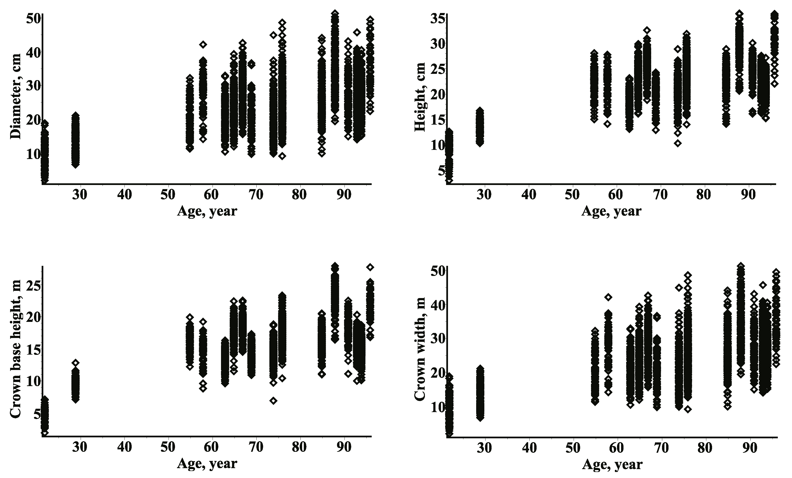
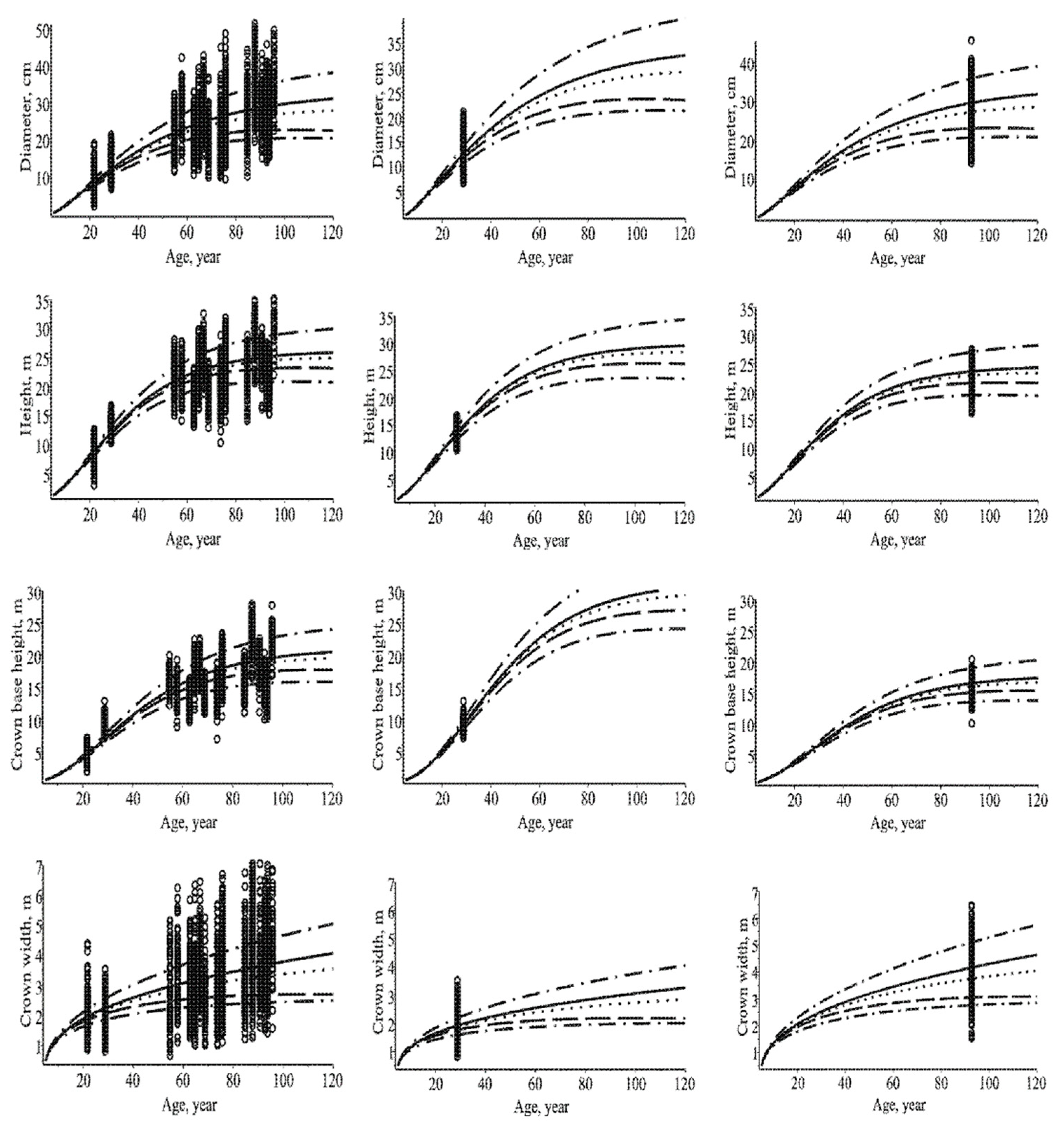
The data used were obtained from 17 permanent experimental Scots pine (Pinus sylvestris L.) stands [6]. The measurements of the diameter at breast height (D), total height (H), crown base height (CH), and crown width (CW) are presented in Figure 1.

The results of the parameter estimates using the NLPSolve procedure in the symbolic algebra system MAPLE [37] are summarized in

Table 1. Estimates of fixed effect parameters.

Model

Parameters of Drift Term

α1

β1

γ1

α2

β2

γ2

α3

β3

γ3

α4

β4

γ4

Fixed

1.3869

0.0269

1.1267

3.1491

0.0441

0.7664

4.7343

0.0392

0.6427

0.3816

3.5 × 10−4

1.0015

Mixed

1.3878

0.0269

1.1265

3.1504

0.0441

0.7663

4.7215

0.0394

0.6436

0.3818

3.5 × 10−4

1.0015

Model

Parameters of Diffusion Term

σ11

σ12

σ13

σ14

σ22

σ23

σ24

σ33

σ34

σ44

Fixed

0.0019

9.0 × 10−4

5.4 × 10−4

0.0016

6.4 × 10−4

5.6 × 10−4

5.9 × 10−4

8.3 × 10−4

0.8 × 10−4

0.0023

Mixed

0.0019

9.6 × 10−4

6.2 × 10−4

0.0015

6.9 × 10−4

5.7 × 10−4

5.7 × 10−4

7.2 × 10−4

1.1 × 10−4

0.0023

Parameters of Random Effects

Mixed

σ1

σ2

σ3

σ4

0.0306

0.1200

0.2240

0.0257

.

3.6. Information Measures

Multivariate data analysis presents a wide range of mathematical and practical problems, particularly in forestry. Datasets sampled from forest stands measurements reflect complex biological systems confronted with diverse multiple interactions and dependencies between tree size variables. Therefore, full-scale analysis of dependencies between size components requires the use of the multivariable information measures. The inference of tree structure evolution, defined by Equation (1), is related to the estimation of the information flow between tree size variables. Entropy is a useful concept to measure the uncertainty in the multivariate stochastic systems and it can be applied to measure multivariate dependences between tree size variables. An information theoretic approach assumes that the development of tree size components will exhibit some dependencies among them, and therefore such statistical dependencies among tree size components can be used to construct the new theoretical growth and yield models. Central to this area is to determine the best relationship of target variable with one another of tree size variables by using an entropy-based technique or more generally to decide whether a subset of multiple tree size components is interdependent. This study will focus on the amount of information transmitted by a set of tree size variables. The simplest information theory measure between two variables is the interaction (mutual) information, which defines the information contained in one variable about another, defined by McGill (1954) [38], can also be interpreted in terms of the Shannon entropy:

$$I(X_s,X_u,t)=H(X_s,t)+H(X_u,t)-H(X_s,X_u,t),1\le s,u\le 4$$

(45)

The definition of the differential Shannon entropy of a stochastic process directly follows that of a continuous random variable. Differential entropy cannot represent the uncertainty of continuous random processes and does not have the point of information. However, mutual information retains its interpretability in the continuous case.

Since the random vector (X₁, X₂, X₃, X₄) is lognormally distributed and for fixed effect scenario the random effects, ${\phi }_i$, $i=1,\dots ,M$, are assumed to be equal its mean value ${\rm E}\left({\phi }_i\right)=0$, ${\mu }_s^i(t)\equiv {\mu }_s(t)$, $1\le s\le 4$, moreover, taking into account stochastic representations of log-skew elliptical random vectors [39], the expressions for univariate and multivariate Shannon entropies (measured in nats) take the following forms [40]:

$$H(X_s,t)\equiv -{\displaystyle \underset{0}{\overset{+\infty }{\int }}f\left(x_s,t|{\hat{\theta }}_s,0\right)}\ln \left(f\left(x_s,t|{\hat{\theta }}_s,0\right)\right)d{x}_s=\frac{1}{2}\ln \left(2\pi e{\sigma }_{ss}(t)\right)+{\mu }_s(t)$$

(46)

$$1\le s\le 4,{\hat{\theta }}_s=\left\{{\hat{\alpha }}_s,{\hat{\beta }}_s,{\hat{\gamma }}_s,{\hat{\sigma }}_{ss}\right\}$$

$$\begin{array}{l}H(X_s,X_u,t)\equiv -{\displaystyle \underset{0}{\overset{+\infty }{\int }}{\displaystyle \underset{0}{\overset{+\infty }{\int }}f\left(x_s,x_u,t|{\hat{\theta }}_{su},0\right)}}\ln \left(f\left(x_s,x_u,t|{\hat{\theta }}_{su},0\right)\right)d{x}_{s}d{x}_u\\ =\frac{1}{2}\ln \left(\left|{\mathsf{\Sigma }}_{su}(t)\right|\right)+\ln \left(2\pi e\right)+{\mu }_s(t)+{\mu }_u(t)\end{array}$$

(47)

$$1\le s,u\le 4,{\hat{\theta }}_{su}=\left\{{\hat{\alpha }}_s,{\hat{\beta }}_s,{\hat{\gamma }}_s,{\hat{\sigma }}_{ss},{\hat{\alpha }}_u,{\hat{\beta }}_u,{\hat{\gamma }}_u,{\hat{\sigma }}_{uu},{\hat{\sigma }}_{su}\right\}$$

$$\begin{array}{l}H(X_s,X_u,X_z,t)\equiv -{\displaystyle \underset{0}{\overset{+\infty }{\int }}{\displaystyle \underset{0}{\overset{+\infty }{\int }}{\displaystyle \underset{0}{\overset{+\infty }{\int }}f\left(x_s,x_u,x_z,t|{\hat{\theta }}_{suz},0\right)}}}\ln \left(f\left(x_s,x_u,x_z,t|{\hat{\theta }}_{suz},0\right)\right)d{x}_{s}d{x}_{u}d{x}_z\\ =\frac{1}{2}\ln \left(\left|{\mathsf{\Sigma }}_{suz}(t)\right|\right)+\frac{3}{2}\ln \left(2\pi e\right)+{\mu }_s(t)+{\mu }_u(t)+{\mu }_z(t)\end{array}$$

(48)

$$1\le s,u,z\le 4,{\hat{\theta }}_{su}=\left\{{\hat{\alpha }}_s,{\hat{\beta }}_s,{\hat{\gamma }}_s,{\hat{\sigma }}_{ss},{\hat{\alpha }}_u,{\hat{\beta }}_u,{\hat{\gamma }}_u,{\hat{\sigma }}_{uu},{\hat{\alpha }}_z,{\hat{\beta }}_z,{\hat{\gamma }}_z,{\hat{\sigma }}_{zz},{\hat{\sigma }}_{su},{\hat{\sigma }}_{sz},{\hat{\sigma }}_{uz}\right\}$$

$$\begin{array}{l}H(X_1,X_2,X_3,X_4,t)\equiv -{\displaystyle \underset{0}{\overset{+\infty }{\int }}{\displaystyle \underset{0}{\overset{+\infty }{\int }}{\displaystyle \underset{0}{\overset{+\infty }{\int }}{\displaystyle \underset{0}{\overset{+\infty }{\int }}f\left(x_1,x_2,x_3,x_4,t|\hat{\theta },0\right)}}}}\ln \left(f\left(x_1,x_2,x_3,x_4,t|{\hat{\theta }}_{suz},0\right)\right)d{x}_{1}d{x}_{2}d{x}_{3}d{x}_4\\ =\frac{1}{2}\ln \left(\left|\mathsf{\Sigma }(t)\right|\right)+2\ln \left(2\pi e\right)+{\mu }_1(t)+{\mu }_2(t)+{\mu }_3(t)+{\mu }_4(t)\end{array}$$

(49)

$$\hat{\theta }=\left\{{\hat{\alpha }}_1,{\hat{\beta }}_1,{\hat{\gamma }}_1,{\hat{\sigma }}_{11},{\hat{\alpha }}_2,{\hat{\beta }}_2,{\hat{\gamma }}_2,{\hat{\sigma }}_{22},{\hat{\alpha }}_3,{\hat{\beta }}_3,{\hat{\gamma }}_3,{\hat{\sigma }}_{33},{\hat{\alpha }}_4,{\hat{\beta }}_4,{\hat{\gamma }}_4,{\hat{\sigma }}_{44},{\hat{\sigma }}_{12},{\hat{\sigma }}_{13},{\hat{\sigma }}_{14},{\hat{\sigma }}_{23},{\hat{\sigma }}_{24},{\hat{\sigma }}_{34}\right\}$$

As we can see from Equation (45), the mutual information, I, is calculated directly by summing the individual entropies and subtracting the joint entropy. Mutual information, I, between two random variables, X_s and X_u, compares the uncertainty of measuring variables jointly with the uncertainty of measuring the two variables independently, identifies nonlinear dependence between two variables [41,42,43], and is non-negative and symmetrical. A generalization of bivariate mutual information to more than two variables have been analyzed in few different scenarios [20,21,41,42,43]. A direct multivariate extension of bivariate mutual information expressed by Equation (45) to n variables X₁, X₂, and X_n is named as the multi-information [44,45], also known as total correlation, and is defined by:

$$\mathsf{\Omega }(X_1,X_2,\dots ,X_n,t)={\displaystyle \sum _{i=1}^{n}H(X_i,t)}-H(X_1,X_2,\dots ,X_n,t).$$

(50)

The multi-information is always non-negative and a near-zero value indicates that the variables are essentially statistically independent. Two special cases of mutual information take the normalized forms, respectively [46,47,48]:

$$N{I}_{\min }(X_s,X_u,t)=\frac{I(X_s,X_u,t)}{\max \left(H(X_s,t),H(X_u,t)\right)},1\le s,u\le 4$$

(51)

$$N{I}_D(X_s,X_u,t)=1-\frac{I(X_s,X_u,t)}{H(X_s,X_u,t)},1\le s,u\le 4$$

(52)

Next normalized variant of the mutual information is provided by the correlation coefficient in the following form [49]:

$$N{I}_C(X_s,X_u,t)=\sqrt{2-\frac{2·I(X_s,X_u,t)}{H(X_s,t)+H(X_u,t)}},1\le s,u\le 4$$

(53)

A simple generalization of the normalized mutual information, defined by Equations (51)–(53), for three variables with the target variable X_s (s = 1, …, 4) takes the following forms:

$$N{I}_{\min }^2(X_s,X_u,X_z,t)=\frac{H(X_s,t)+H(X_u,X_z,t)-H(X_s,X_u,X_z,t)}{\max \left(H(X_s,t),H(X_u,X_z,t)\right)},u,z\in \left\{1,2,3,4\right\}/\left\{s\right\},$$

(54)

$$N{I}_D^2(X_s,X_u,X_z,t)=\frac{H(X_s,t)+H(X_u,X_z,t)-H(X_s,X_u,X_z,t)}{H(X_s,X_u,X_z,t)},u,z\in \left\{1,2,3,4\right\}/\left\{s\right\}$$

(55)

$$\begin{array}{c}N{I}_C^2(X_s,X_u,X_z,t)=\sqrt{2-\frac{2\left(H(X_s,t)+H(X_u,X_z,t)-H(X_s,X_u,X_z,t)\right)}{H(X_s,t)+H(X_u,X_z,t)}},\\ u,z\in \left\{1,2,3,4\right\}/\left\{s\right\}\end{array}$$

(56)

Generalized forms of mutual information to more than two variables are called interaction information [21,47]. The relationship between multi-information and interaction information for the trivariate and 4-variate cases are defined in the following forms [21]:

$$I(X_1,X_2,X_3,t)={\displaystyle \sum _{s>u}I(X_s,X_u,t)}-\mathsf{\Omega }(X_1,X_2,X_3,t),$$

(57)

$$I(X_1,X_2,X_3,X_4,t)={\displaystyle \sum _{z>s>u}I(X_s,X_u,X_z,t)}-{\displaystyle \sum _{s>u}I(X_s,X_u)}+\mathsf{\Omega }(X_1,X_2,X_3,X_4,t).$$

(58)

Providing that the target variable X_s ($1\le s\le 4$) is added to the set of ${\nu }_{n-1}=\left(X_1,....,X_{s-1},X_{s+1},....,X_n\right)$ variables, the differential interaction information [21,47] is defined as:

$${\Delta }_n\left({\nu }_{n-1};X_s,t\right)=I\left({\nu }_n,t\right)-I\left({\nu }_{n-1},t\right),{\nu }_n=\left(X_1,\dots ,X_n\right)$$

(59)

In consequence of Equations (45), (46) and (59), the deltas for two variables ${\nu }_2=\left(X_s,X_u\right)$, $1\le s\le 4$, $u\in \left\{1,2,3,4\right\}/\left\{s\right\}$ (the target variable X_s) are defined as:

$${\Delta }_2\left({\nu }_1;X_s,t\right)=I\left({\nu }_2,t\right)-H\left(X_s,t\right),{\nu }_2=\left(X_s,X_u\right),{\nu }_1=\left(X_u\right)$$

(60)

for three variables ${\nu }_3=\left(X_s,X_u,X_z\right)$, $1\le s\le 4$, $u,z\in \left\{1,2,3,4\right\}/\left\{s\right\}$ (the target variable X_s) are defined as:

$${\Delta }_3\left({\nu }_2;X_s,t\right)=I\left({\nu }_3,t\right)-I\left({\nu }_2,t\right),{\nu }_2=\left(X_u,X_z\right)$$

(61)

for four variables ${\nu }_4=\left(X_s,X_u,X_z,X_y\right)$ $1\le s\le 4$, $u,z,y\in \left\{1,2,3,4\right\}/\left\{s\right\}$ (the target variable X_s) are defined as:

$${\Delta }_4\left({\nu }_3;X_s,t\right)=I\left({\nu }_4,t\right)-I\left({\nu }_3,t\right)$$

(62)

4. Discussion

Traditionally, the used statistical metrics for goodness-of-fit linear and nonlinear regression models mostly reflect only fitting criteria (not goodness of fit), which was used in an optimization process to get the best-fit parameters. For example, the coefficient of determination cannot determine whether the parameter estimates and predictions are biased. Similarly, a low value of the coefficient of determination can produce a good model. Consequently, the best metrics possessed model is not necessarily the one that fits best the data. 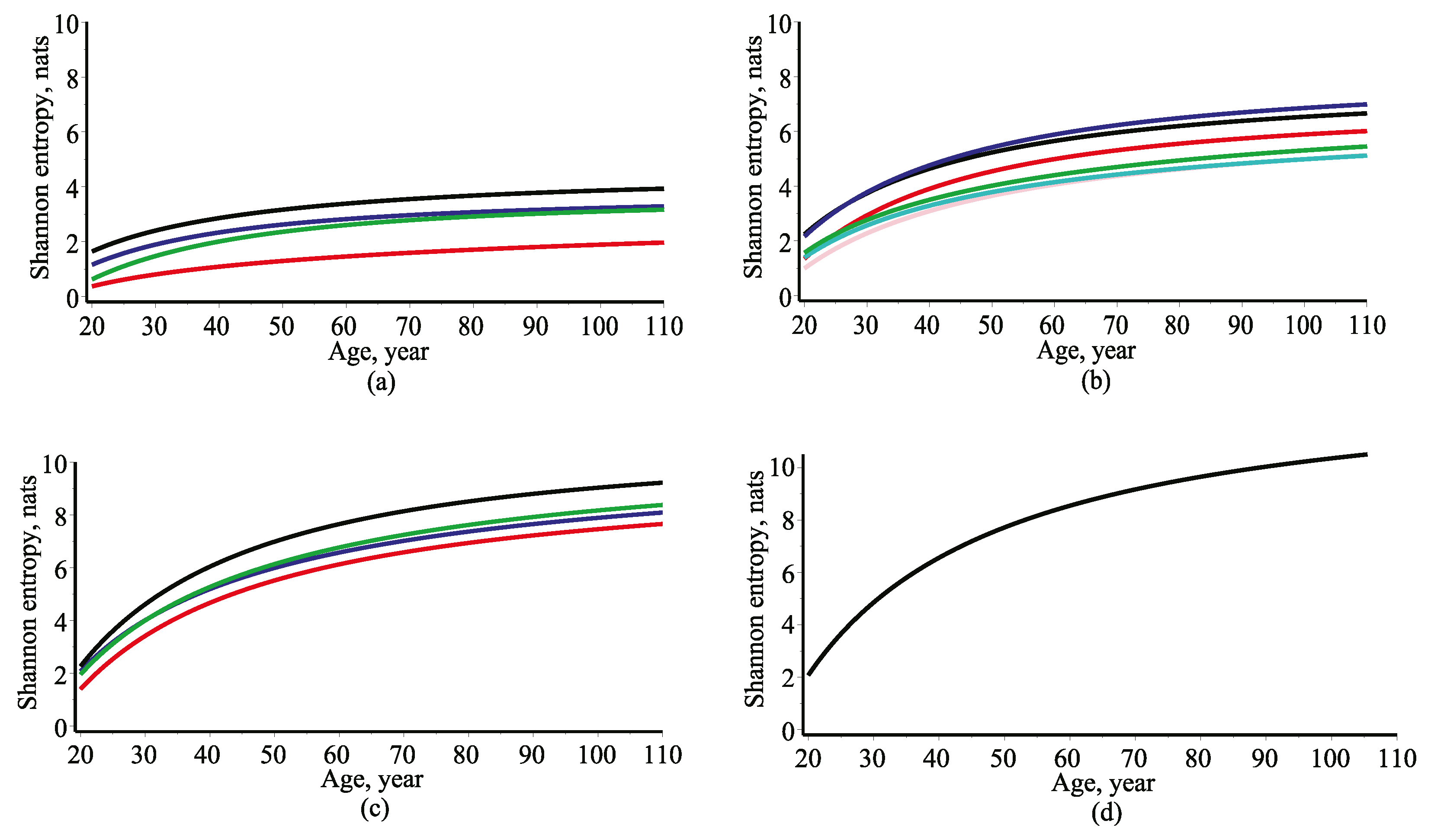Evaluation of the model fit within information measures relies on the detection of variable dependence, estimation of the significance of such dependence and inference of the functional form of the dependence [21,47]. Moreover, information measures operate on probability distributions rather than directly on data. In this study, the functional forms of inter-variable relationships are deducible using marginal densities (Equations (7), (8), (14), (15), (18) and (19)) of the 4-variate probability density function which is a solution of a diffusion process defined by Equation (1). In this study, the problem of inter-variable dependencies and correlations of new developed functional forms of tree size variable dynamic is analyzed by using entropy-based measures like interaction information, normalized interaction information, multi-information and differential interaction information (see Equations (45)–(62)). The Shannon entropies of the evolution of tree diameter, height, crown base height and crown width in univariate, bivariate, trivariate and four-variate cases are graphically charted in Figure 2.

It is evident that, to some extent, entropy can be viewed as the amount of information that can be gathered through observed dataset. It is understandable that the lower is the Shannon entropy of the tree size variable the less information about the evolution of a tree we are missing and providing more information about the tree development. Figure 2 shows that for all scenarios (univariate, bivariate, trivariate and four-variate) the Shannon entropy increases against the time (age). Hence, an information available about the tree development is actually losing with acceding a tree age. Moreover, the differences of the Shannon entropy (uncertainty measures) between different scenarios of tree size variables can be interpreted as an information gain or loss. It is important to note, if a tree size variable have a small single uncertainty measure, then contribution to the multivariate entropy turns out to be negligible. The univariate probability density function of the diameter, defined by Equations (7) and (8), produced the supreme entropy relationship whereas the univariate probability density function of the crown width produced the least entropy relationship. The bivariate probability density function of the diameter and height, defined by Equations (14) and (15), produced the supreme entropy relationship whereas the bivariate probability density function of the crown base height and crown width produced the least entropy relationship. Lastly, the trivariate probability density function of the diameter, height and crown base height, defined by Equations (18) and (19), produced the supreme entropy relationship whereas the trivariate probability density function of the height, crown base height and crown width produced the minimal entropy relationship.

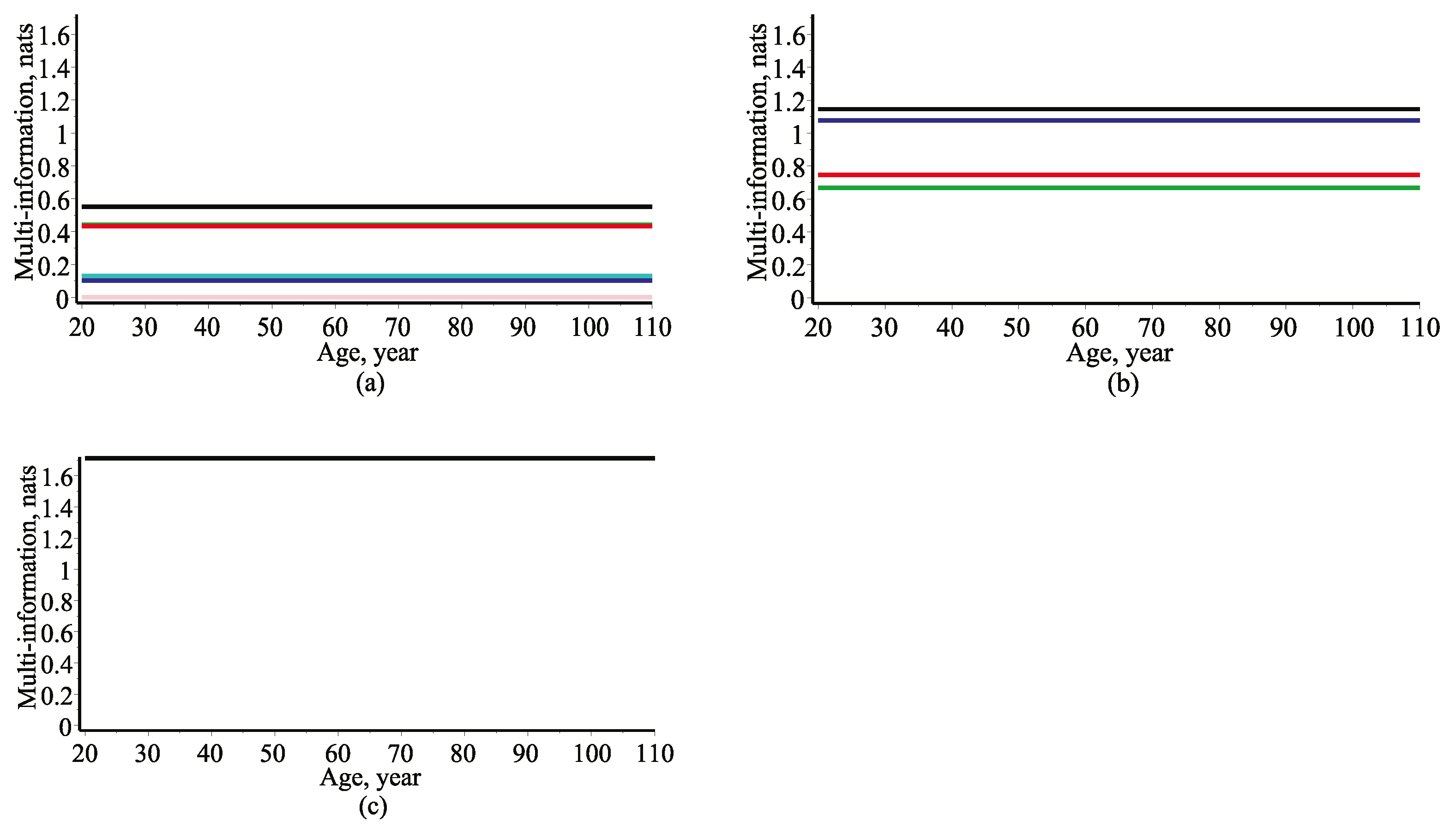
A complex way of quantifying statistical dependencies between tree size variables comes from the definition of multi-information, which is defined as the difference between the sum of single entropies for each tree size variables and the joint entropy of all tree size variables. The multi-information defined by Equation (55) quantifies the total amount of information carried by correlations between the variables. As a measure of overall multivariable dependence or redundancy, this quantity goes to zero if all variables are independent. The information measure defined by Equations (45) and (50) is named as the total multi-information of two and n random variables, respectively. Figure 3 shows that multi-information is positive, remains stable against the age and gathers bigger values by increasing the number of tree size variables. It is obvious that the multi-information is equal to the mutual information when n = 2. If we range all relationships by using multi-information measure, then, for example, examine Figure 3 we could choose the most important predictor variables for quantifying other response variable. It follows that for a single response tree size variable—diameter (black, blue and green curves) the superior relationship could be defined using a height (black—diameter and height) as a predictor variable; for the height (black, red and cyan curves) the superior relationship could be defined using a diameter (black—diameter and height); for the crown base height (blue, cyan and pink curves) the superior relationship could be defined using height (cyan—height and crown base height); and for the crown width (green, pink and cyan curves) the superior relationship could be defined using a diameter (green—diameter and crown diameter). However, such ranging procedure is not successful, as the low joint entropy value of n variables will also produce low the value of multi-information even if the all the variables are perfectly related. Figure 3 shows that the amount of multi-information is apparently constant via age.

The concept of causality is commonly understandable as the capacity of one variable to influence another. As was noted by Wiener [50] for two simultaneously measured variables, ‘if we can predict the first variable better by using the past information from the second one than by using the information without it, then we call the second variable causal to the first one’. In Wiener’s formulation, the causality is a statistical concept that is based on prediction. Consequently, the best-ranked relationship is not necessarily the one that fits best the data, but that carries superior causality information. Recognizing the statement about causality as an information [51] about the effect of nonlinear relationship we can examine and compare new developed nonlinear relationships by using intersection information measures defined by Equations (45) and (51)–(62). Modeling of the evolution of tree size variables requires better understanding which predictor exerts primary control on response tree size variable. Mutual information quantifies the amount of information that one tree size variable reveals about another and thus the strength of their codependency. Interconnecting causality with mutual information we can measure how much knowing one of these tree size variables reduces uncertainty about the other. If two tree size variables are independent, then knowing single tree size variable does not give any information about another tree size variable and vice versa, so their mutual information is zero. Unfortunately, the value of mutual information depends on the absolute magnitude of joint entropy between the two chosen tree size variables and is not appropriate to use directly for relative comparisons. Therefore, for the ranging of all developed models is advisable to use normalized interaction measures, defined by Equations (51)–(56). The higher normalized information measure values of the bivariate and trivariate mutual information (Equations (51), (53), (54) and (56)) show stronger relationship. The normalized mutual information interpreted in typical distance metric form (see Equations (52) and (55)) is closer to zero in case of a stronger similarity. 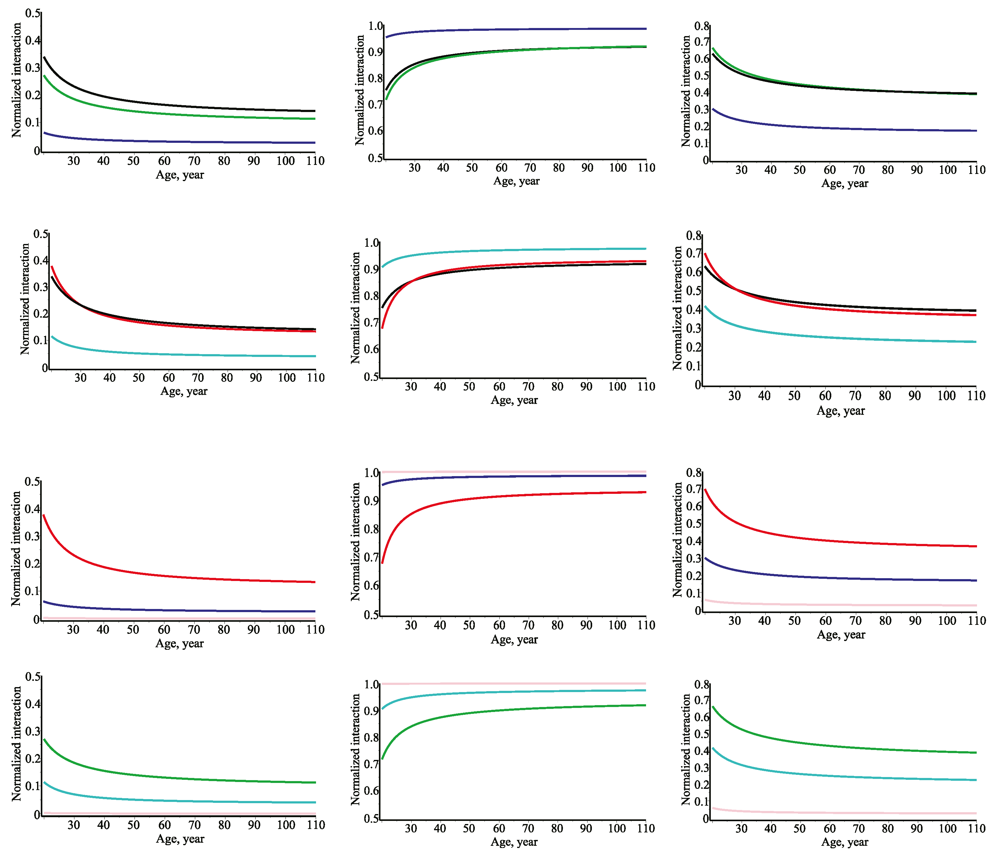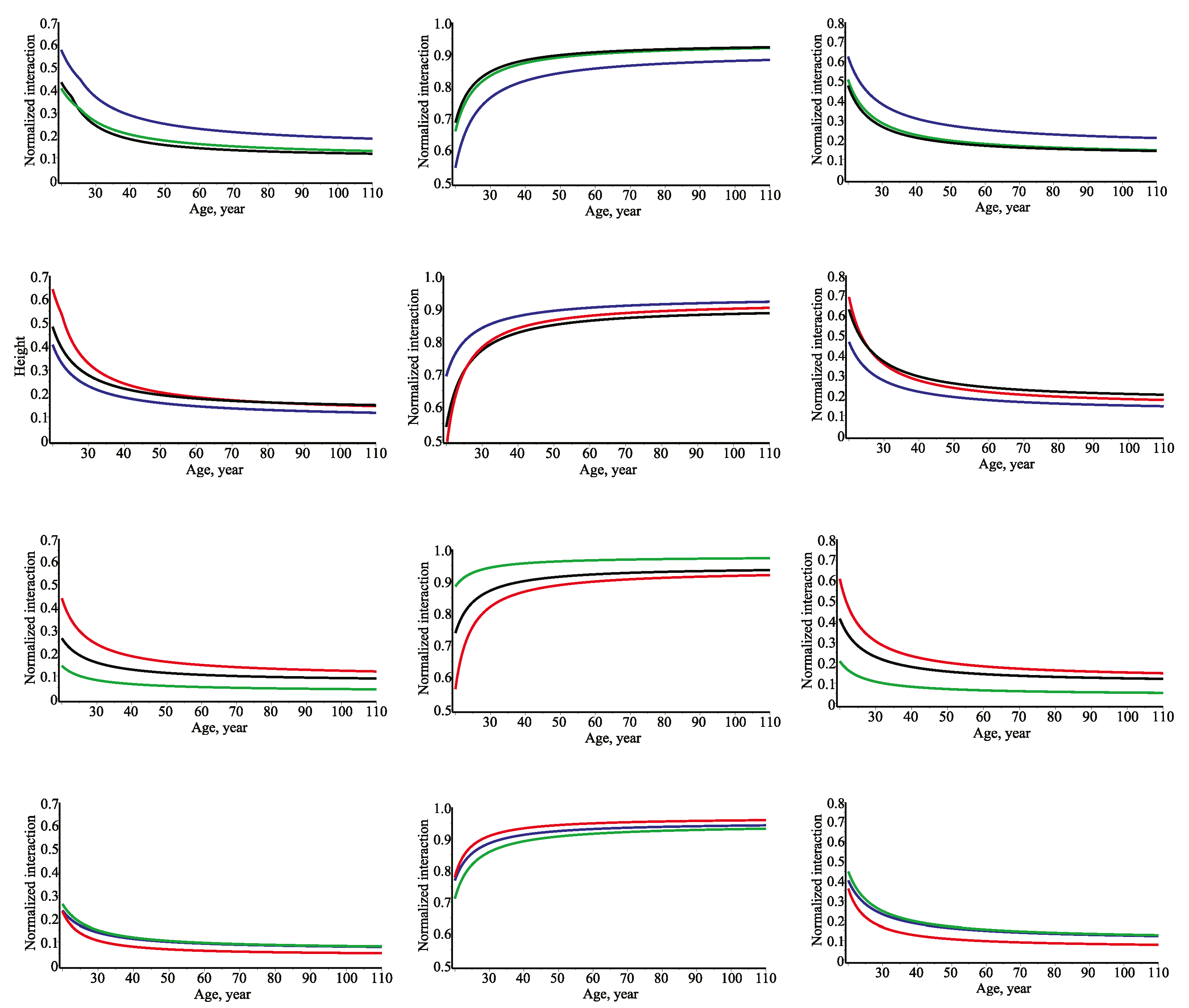Figure 4 presents the evolution of the bivariate normalized mutual information defined by Equations (51)–(56). Eventually, the results presented in Figure 4, provide strong evidence that information measures are powerful tools to quantify and explain the relevance of different nonlinear relationships for tree size variables modeling. It follows, that for the quantifying tree diameter relationship against a single predictor variable it must be the crown width or the height, as the corresponding bivariate normalized mutual information curves are sufficiently close or intersects. Following this overall result for the quantifying tree height relationship against a single predictor variable it must be the crown base height or the diameter, as the corresponding bivariate normalized mutual information curves are sufficiently close or intersects. For the quantifying tree crown base height relationship against a single predictor variable it must be the height and, eventually, for the quantifying tree crown base height relationship best a single predictor variable must be the diameter.

The evolution of the trivariate normalized mutual information defined by Equations (54)–(56) is presented in Figure 5. In parallel with bivariate normalized mutual information scenario we can compare nonlinear relationships using trivariate normalized mutual information (see Equations (54)–(56)). Consequently, for the quantifying of tree diameter relationship against two predictor variables it must be the crown base height and crown width. For the quantifying of tree height relationship against two predictor variables it must be the diameter and crown base height. Moreover, for the quantifying of tree crown base height relationship against two predictor variables it must be the height and crown width. Eventually, for the quantifying of tree crown width relationship the best two predictor variables must be the diameter and crown base height.

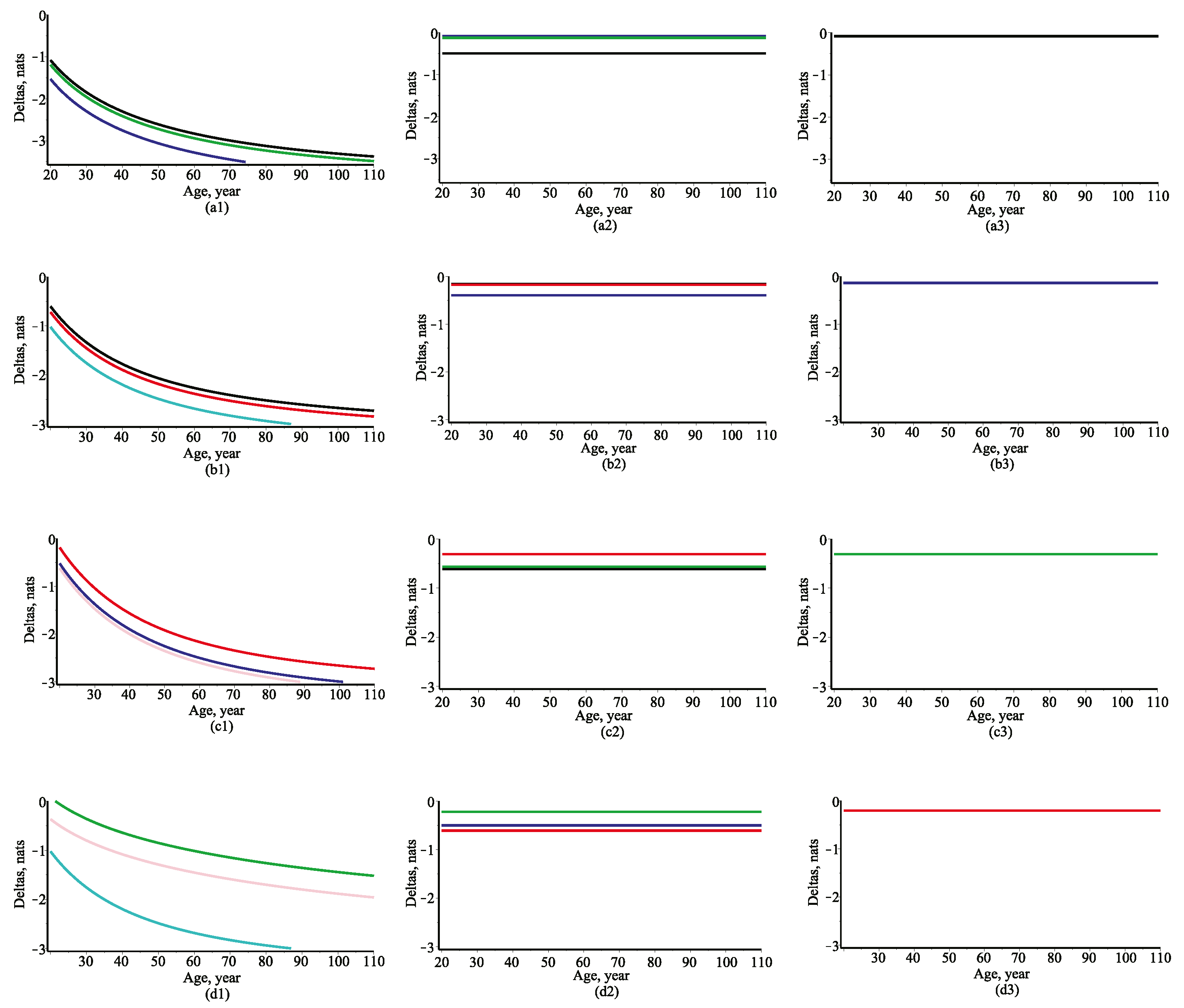
Given the initial state of the tree size variables, the solution of the SDE (1) determines the dynamic of the univariate, marginal and conditional probability density functions of state variables. These density functions of tree size variables are updated at each age. The dynamic of the univariate marginal and conditional density functions of tree size variables provides the updated prediction by using the mean and the conditional mean trend. For the test on predictive capacity of new derived nonlinear relationships previously were discussed the concepts of the normalized mutual information. To make SDE models comparison more precise, the difference of the intersection information (deltas) defined by Equations (58)–(62) prevails over previous discussed decisions. Figure 6 presents the evolution of the difference of the intersection information (deltas). For tree growth modeling the general problem is to guarantee the maximum degree of dependence to be considered and to determine the number of the best predictor variables involved. The three non-linear scenarios (one, two and three predictors) for the mean trend of a response variable were developed in the present study. The further discussion deals with the adequacy of the deltas defined by Equations (59)–(62) in describing the dependence and causality of the tree size variables. The non-linear models showed that more of predictor variables is included the higher deltas value is achieved. Therefore, the nonlinear models with three predictors (see Figure 6 the third column) provided the best reveal of dependence of all response variables (diameter, height, crown base height and crown width) due to the higher values of deltas than other models (one or two predictors). The shape of the deltas curves in the first column of Figure 6 showed that height reveals the most part of dependence between diameter and other tree size variables (but remains very close result when used crown width as a predictor variable). The diameter reveals the most part of dependence between height and other tree size variables; the height reveals the most part of dependence between crown base height and other tree size variables; eventually, the diameter reveals the most part of dependence between crown width and other tree size variables.

In the second column of Figure 6 the deltas curve showed that the height and crown width reveal the most part of dependence between diameter and other two tree size variables. The diameter and crown base height reveal the most part of dependence between height and other two tree size variables; the height and crown width reveal the most part of dependence between crown base height and other two tree size variables; eventually, the diameter and crown base height reveal the most part of dependence between crown width and other two tree size variables.

The ranking and selection of the mean tree size curves $m_s^i(t)$, $m_s^i(t,x_u)$, $m_s^i(t,x_u,x_z)$ and $m_s^i(t,x_u,x_z,x_y)$ can be alternately performed using basic statistical measures, for example, mean bias (MB), mean absolute bias (MAB), root mean square error (RMSE), adjusted coefficient of determination R², and Akaike’s information criterion (AIC) [6,17]. Statistical measures and the ranking for both fixed- and mixed effects scenarios presented in

Table 2. Goodness-of fit numerical statistical measures for the fixed- and mixed effects scenario models.

Predictors	Fixed Effect Scenario					Mixed Effect Scenario
	B (Rank)	MAB (Rank)	RMSE Rank)	R2 (Rank)	AIC (Rank)	MB (Rank)	MAB (Rank)	RMSE (Rank)	R2 (Rank)	AIC (Rank)
Diameter
(t)	−0.619 (7)	5.472 (8)	6.765 (8)	0.355 (8)	26967 (8)	−0.837 (8)	4.823 (8)	5.869 (8)	0.515 (8)	26306 (8)
(t,H)	0.097 (2)	3.350 (5)	4.292 (5)	0.741 (5)	24852 (5)	−0.048 (1)	2.956 (6)	3.784 (6)	0.798 (6)	24267 (6)
(t,CH)	−0.012 (1)	4.786 (7)	5.951 (7)	0.501 (7)	26374 (7)	−0.493 (6)	4.491 (7)	5.570 (7)	0.563 (7)	26068 (7)
(t,CW)	−0.734 (8)	3.380 (6)	4.304 (6)	0.739 (6)	24864 (6)	−0.551 (7)	2.852 (5)	3.744 (5)	0.803 (5)	24217 (5)
(t,H,CH)	−0.178 (4)	2.887 (4)	3.711 (4)	0.806 (4)	24184 (4)	−0.073 (2)	2.664 (4)	3.470 (4)	0.830 (4)	23974 (4)
(t,H,CW)	−0.165 (3)	2.204 (2)	2.892 (2)	0.881 (2)	23019 (2)	−0.083 (4)	1.974 (2)	2.623 (2)	0.903 (2)	22567 (2)
(t,CH,CW)	−0.223 (6)	2.707 (3)	3.584 (3)	0.819 (3)	24018 (3)	−0.261 (5)	2.600 (3)	3.446 (3)	0.833 (3)	23838 (3)
(t,H,CH,CW)	−0.217 (5)	2.135 (1)	2.797 (1)	0.890 (1)	22870 (1)	−0.081 (3)	1.942 (1)	2.590 (1)	0.906 (1)	22515 (1)
Height
(t)	−0.376 (7)	3.038 (8)	3.766 (8)	0.497 (8)	24238 (8)	−0.351 (8)	1.984 (8)	2.561 (8)	0.767 (8)	22433 (8)
(t,D)	−0.257 (6)	1.883 (5)	2.350 (5)	0.804 (5)	22045 (5)	−0.180 (5)	1.380 (4)	1.752 (4)	0.891 (4)	20680 (4)
(t,CH)	0.166 (5)	1.676 (4)	2.114 (4)	0.841 (4)	21553 (4)	−0.088 (4)	1.521 (5)	1.929 (5)	0.868 (5)	21129 (5)
(t,CW)	−0.461 (8)	2.709 (7)	3.349 (7)	0.602 (7)	23696 (7)	−0.331 (7)	1.703 (7)	2.235 (7)	0.823 (6–7)	21815 (6)
(t,D,CH)	0.065 (2)	1.029 (2)	1.312 (1–2)	0.939 (1–2)	19336 (1)	−0.048 (2)	0.939 (2)	1.215 (2)	0.948 (1–2)	18981 (1–2)
(t,D,CW)	−0.118 (4)	2.189 (6)	2.857 (6)	0.710 (6)	22962 (6)	−0.203 (6)	1.668 (6)	2.234 (6)	0.823 (6–7)	21819 (7)
(t,CH,CW)	0.060 (1)	1.293 (3)	1.678 (3)	0.900 (3)	20482 (3)	−0.082 (3)	1.219 (3)	1.592 (3)	0.910 (3)	20240 (3)
(t,D,CH,CW)	0.067 (3)	1.027 (1)	1.312 (1–2)	0.939 (1–2)	19345 (2)	−0.046 (1)	0.936 (1)	1.213 (1)	0.948 (1–2)	18981 (1–2)
Crown base height
(t)	−0.711 (7)	2.575 (8)	3.042 (8)	0.488 (8)	23243 (8)	−0.299 (7)	1.329 (4)	1.722 (5)	0.836 (5)	20595 (5)
(t,D)	−0.685 (6)	2.231 (6)	2.689 (6)	0.600 (6)	22674 (6)	−0.254 (6)	1.371 (8)	1.748 (6)	0.831 (6)	20668 (6)
(t,H)	−0.470 (4)	1.353 (4)	1.683 (4)	0.843 (4)	20492 (4)	−0.126 (3)	1.029 (3)	1.342 (3)	0.900 (3)	19437 (3)
(t,CW)	−0.724 (8)	2.558 (7)	3.025 (7)	0.494 (7)	23223 (7)	−0.300 (8)	1.330 (5)	1.718 (4)	0.837 (4)	20590 (4)
(t,D,H)	−0.369 (3)	1.154 (2)	1.456 (1)	0.883 (1)	19822 (2)	−0.135 (4)	1.375 (7)	1.770 (7)	0.827 (7)	20735 (7)
(t,D,CW)	−0.506 (5)	2.012 (5)	2.490 (5)	0.657 (5)	22321 (5)	−0.191 (5)	1.362 (7)	1.797 (8)	0.821 (8)	20805 (8)
(t,H,CW)	−0.326 (1–2)	1.181 (3)	1.514 (3)	0.873 (3)	20004 (3)	−0.081 (2)	0.948 (2)	1.264 (2)	0.912 (2)	19166 (2)
(t,D,H,CW)	−0.326 (1–2)	1.146 (1)	1.461 (2)	0.882 (2)	19485 (1)	−0.078 (1)	0.933 (1)	1.243 (1)	0.915 (1)	19096 (1)
Crown width
(t)	−0.009 (4)	0.884 (8)	1.108 (8)	0.180 (8)	18540 (8)	−0.091 (8)	0.834 (8)	1.038 (8)	0.281 (8)	18237 (7)
(t,D)	0.044 (8)	0.542 (4)	0.700 (4)	0.673 (4)	16402 (4)	−0.018 (1)	0.506 (4)	0.660 (4)	0.710 (4)	16129 (4)
(t,H)	0.036 (7)	0.770 (6)	0.983 (6)	0.355 (6)	17980 (6)	−0.055 (6)	0.720 (6)	0.916 (6)	0.440 (6)	17660 (6)
(t,CH)	0.001 (1)	0.878 (7)	1.102 (7)	0.189 (7)	18515 (7)	−0.090 (7)	0.831 (7)	1.037 (7)	0.282 (7)	18238 (8)
(t,D,H)	0.024 (6)	0.498 (3)	0.650 (3)	0.718 (3)	16058 (2)	−0.025 (4)	0.481 (3)	0.631 (3)	0.734 (3)	15929 (3)
(t,D,CH)	0.007 (2–3)	0.491 (2)	0.640 (1)	0.726 (1–2)	15989 (1)	−0.020 (2)	0.471 (2)	0.621 (2)	0.742 (2)	15859 (2)
(t,H,CH)	−0.010 (5)	0.667 (5)	0.855 (5)	0.512 (5)	17339 (5)	−0.040 (5)	0.638 (5)	0.835 (5)	0.535 (5)	17234 (5)
(t,D,H,CH)	0.007 (2–3)	0.490 (1)	0.641 (2)	0.726 (1–2)	16293 (3)	−0.021 (3)	0.469 (1)	0.618 (1)	0.745 (1)	15842 (1)

. Therefore, from a statistical point of view (see Table 2), for the fixed effects scenario all relationships attained lower values of statistical indexes than the mixed effects scenario models.

New developed nested statistical models, defined as a set of probability distributions on the sample space (dataset), support growth and yield modeling by facilitating individualized outcomes conditional on predictor variables. The goodness-of-fit of a model to dataset evaluated through the use of numerical statistical measures and presented in Table 2 provides summary measures of the overall accuracy of the predictions. The goodness-of-fit of new developed models to data assessed by using numerical statistical measures MB, MAB, RMSE, R² and AIC presented in Table 2, and information measures defined by Equations (45)–(62) and visualized in Figure 1, Figure 2, Figure 3, Figure 4 and Figure 5 showed very similar results. This study presents that the interaction information measure approach is particularly powerful, but has less general applicability because of the complicated calculations required, which are not always presently solvable.

Forests statisticians who use mathematics but are not completely at ease with abstract mathematical notations and formulas presented in Equations (1)–(62) can often better understand the new derived mathematical models if these models are visually embodiment. Using the univariate marginal distributions (Equations (7) and (8)), Figure 7 shows the mean, mode, median and both quartiles trends via the mean stand age (in the mixed-effect scenario for randomly selected two stands). The implementation of abstract mathematical Equations (9)–(12) visually reveals nonsymmetry that was not apparent from the observed discrete datasets. Just such a hidden nonsymmetry, disclosed by visualization, confirmed the fact that tree size variables are positively skewed.

References

1. Sharma, R.P.; Vacek, Z.; Vacek, S.; Kučera, M. A Nonlinear Mixed-Effects Height-to-Diameter Ratio Model for Several Tree Species Based on Czech National Forest Inventory Data. Forests 2019, 10, 70. [Google Scholar] [CrossRef]
2. Gangying, H.; Zhang, G.; Zhao, Z.; Yang, Y. Methods of Forest Structure Research: A Review. Curr. For. Rep. 2019, 5, 69–78. [Google Scholar]
3. Román-Román, P.; Serrano-Pérez, J.J.; Torres-Ruiz, F. A Note on Estimation of Multi-Sigmoidal Gompertz Functions with Random Noise. Mathematics 2019, 7, 541. [Google Scholar] [CrossRef]
4. Nucci, M.C.; Sanchini, G. Noether Symmetries Quantization and Superintegrability of Biological Models. Symmetry 2016, 8, 155. [Google Scholar] [CrossRef]
5. Garcıa, O. Forest Stands as Dynamical Systems: An Introduction. Mod. Appl. Sci. 2013, 7, 32–38. [Google Scholar] [CrossRef]
6. Rupšys, P.; Petrauskas, E. A Linkage among Tree Diameter, Height, Crown Base Height, and Crown Width 4-variate Distribution and Their Growth Models: A 4-variate Diffusion Process Approach. Forests 2017, 8, 479. [Google Scholar] [CrossRef]
7. Rupšys, P.; Petrauskas, E. A New Paradigm in Modelling the Evolution of a Stand via the Distribution of Tree Sizes. Sci. Rep. 2017, 7, 12154. [Google Scholar] [CrossRef] [PubMed]
8. Rupšys, P. Modeling Dynamics of Structural Components of Forest Stands Based on Trivariate Stochastic Differential Equation. Forests 2019, 10, 506. [Google Scholar] [CrossRef]
9. Duan, G.; Gao, Z.; Wang, Q.; Fu, L. Comparison of Different Height–Diameter Modelling Techniques for Prediction of Site Productivity in Natural Uneven-Aged Pure Stands. Forests 2018, 9, 29. [Google Scholar] [CrossRef]
10. Román-Román, P.; Serrano-Pérez, J.J.; Torres-Ruiz, F. Some Notes about Inference for the Lognormal Diffusion Process with Exogenous Factors. Mathematics 2018, 6, 85. [Google Scholar] [CrossRef]
11. Rupšys, P.; Petrauskas, E. Evolution of Bivariate Tree Diameter and Height Distribution via Stand Age: Von Bertalanffy Bivariate Diffusion Process Approach. J. Forest Res. Jap. 2019, 24, 16–26. [Google Scholar] [CrossRef]
12. Di Crescenzo, A.; Paraggio, P. Logistic Growth Described by Birth-Death and Diffusion Processes. Mathematics 2019, 7, 489. [Google Scholar] [CrossRef]
13. Rupšys, P. Time Delay Stochastic Logistic Growth Laws in Single-Species Population Growth Modeling. In Proceedings of the 4th WSEAS International Conference on Mathematical Biology and Ecology, Acapulco, Mexico, 25–27 January 2008; pp. 29–34. [Google Scholar]
14. Muñoz-Cobo, J.L.; Berna, C. Chemical Kinetics Roots and Methods to Obtain the Probability Distribution Function Evolution of Reactants and Products in Chemical Networks Governed by a Master Equation. Entropy 2019, 21, 181. [Google Scholar] [CrossRef]
15. Visalga, G.; Rupšys, P.; Petrauskas, E. Influence of Noise on Decay Predictions in Standing Trees. AIP Conf. Proc. 2017, 1895, 030006. [Google Scholar]
16. Cai, W.; Pan, J. Stochastic Differential Equation Models for the Price of European CO2 Emissions Allowances. Sustainability 2017, 9, 207. [Google Scholar] [CrossRef]
17. Rupšys, P. New Insights into Tree Height Distribution Based on Mixed Effects Univariate Diffusion Processes. PLoS ONE 2016, 11, e0168507. [Google Scholar] [CrossRef]
18. Rupšys, P. The Use of Copulas to Practical Estimation of Multivariate Stochastic Differential Equation Mixed Effects Models. AIP Conf. Proc. 2015, 1684, 080011. [Google Scholar]
19. Ju, B.; Zhang, H.; Liu, Y.; Pan, D.; Zheng, P.; Xu, L.; Li, G. A Method for Detecting Dynamic Mutation of Complex Systems Using Improved Information Entropy. Entropy 2019, 21, 115. [Google Scholar] [CrossRef]
20. Sakhanenko, N.A.; Galas, D.J. Biological Data Analysis as an Information Theory Problem: Multivariable Dependence Measures and the Shadows Algorithm. J. Comput. Biol. 2015, 22, 1005–1024. [Google Scholar] [CrossRef] [Green Version]
21. Galas, D.J.; Sakhanenko, N.A. Symmetries among Multivariate Information Measures Explored Using Möbius Operators. Entropy 2019, 21, 88. [Google Scholar] [CrossRef]
22. Hara, T. A Stochastic Model and the Moment Dynamics of the Growth and Size Distribution in Plant Populations. J. Theor. Biol. 1984, 109, 173–190. [Google Scholar] [CrossRef]
23. Kohyama, T.; Hara, T. Frequency Distribution of Tree Growth Rate in Natural Forest Stands. Ann. Bot. London 1989, 64, 47–57. [Google Scholar] [CrossRef]
24. Kohyama, T.S.; Potts, M.D.; Kohyama, T.I.; Kassim, A.R.; Ashton, P.S. Demographic Properties Shape Tree Size Distribution in a Malaysian Rain Forest. Am. Nat. 2015, 185, 367–379. [Google Scholar] [CrossRef] [Green Version]
25. Hozumi, K.; Shinozaki, K.; Tadaki, Y. Studies on the Frequency Distribution of the Weight of Individual Trees in a Forest Stand I. A New Approach Toward the Analysis of the Distribution Function and the-3/2th Power Distribution. Jpn. J. Ecol. 1968, 18, 10–20. [Google Scholar]
26. Rupšys, P. Generalized Fixed-Effects and Mixed-Effects Parameters Height–Diameter Models with Diffusion Processes. Int. J. Biomath. 2015, 8, 1550060. [Google Scholar] [CrossRef]
27. Rupšys, P. Height–Diameter Models with Stochastic Differential Equations and Mixed-Effects Parameters. J. For. Res. Jap. 2015, 20, 9–17. [Google Scholar] [CrossRef]
28. Rupšys, P. Stochastic Mixed-Effects Parameters Bertalanffy Process, with Applications to Tree Crown Width Modeling. Math. Probl. Eng. 2015, 2015, 375270. [Google Scholar] [CrossRef]
29. Li, C. Maximum-Likelihood Estimation for Diffusion Processes via Closed-Form density Expansions. Ann. Statist. 2013, 41, 1350–1380. [Google Scholar] [CrossRef]
30. García, O. Estimating Reducible Stochastic Differential Equations by Conversion to a Least-Squares Problem. Comput. Stat. 2019, 34, 23–46. [Google Scholar] [CrossRef]
31. Picchini, U.; Gaetano, A.; Ditlevsen, S. Stochastic Differential Mixed-Effects Models. Scand. J. Stat. 2010, 37, 67–90. [Google Scholar] [CrossRef]
32. Itô, K. On stochastic processes. Jap. J. Math. 1942, 18, 261–301. [Google Scholar] [CrossRef]
33. Uhlenbeck, G.E.; Ornstein, L.S. On the Theory of Brownian Motion. Phys. Rev. 1930, 36, 823–841. [Google Scholar] [CrossRef]
34. Garvey, P.R.; Book, S.A.; Covert, R.P. Probability Methods for Cost Uncertainty Analysis: A Systems Engineering Perspective, 2nd ed.; Chapman and Hall/CRC: New York, NY, USA, 2016. [Google Scholar]
35. Garvey, P.R. Garvey: A Family of Joint Probability Models for Cost and Schedule Uncertainties. J. Cost Anal. 1995, 12, 156–200. [Google Scholar] [CrossRef]
36. Joe, H. Accuracy of Laplace Approximation for Discrete Response Mixed Models. Comput. Stat. Data An. 2008, 52, 5066–5074. [Google Scholar] [CrossRef]
37. Monagan, M.B.; Geddes, K.O.; Heal, K.M.; Labahn, G.; Vorkoetter, S.M.; Mccarron, J. Maple Advanced Programming Guide; Maplesoft: Waterloo, ON, Canada, 2007. [Google Scholar]
38. McGill, W. Multivariate Information Transmission. Psychometrika 1954, 19, 97–116. [Google Scholar] [CrossRef]
39. Marchenko, Y.V.; Genton, M.G. Multivariate Log-Skew-Elliptical Distributions with Applications to Precipitation Data. Environmetrics 2010, 21, 318–340. [Google Scholar] [CrossRef]
40. De Queiroz, M.M.; Silva, R.W.; Loschi, R.H. Shannon Entropy and Kullback–Leibler Divergence in Multivariate Log Fundamental Skew-Normal and Related Distributions. Can. J. Stat. 2016, 44, 219–237. [Google Scholar] [CrossRef]
41. Eskandarzadeh, M.; Di Crescenzo, A.; Tahmasebi, S. Cumulative Measure of Inaccuracy and Mutual Information in k-th Lower Record Values. Mathematics 2019, 7, 175. [Google Scholar] [CrossRef]
42. Li, W. Mutual Information Functions Versus Correlation Functions. J. Stat. Phys. 1990, 60, 823–837. [Google Scholar] [CrossRef]
43. Wing, S.; Johnson, J.R. Applications of Information Theory in Solar and Space Physics. Entropy 2019, 21, 140. [Google Scholar] [CrossRef]
44. Watanabe, S. Information Theoretical Analysis of Multivariate Correlation. IBM J. Res. Dev. 1960, 4, 66–82. [Google Scholar] [CrossRef]
45. Galas, D.J.; Dewey, G.; Kunert-Graf, J.; Sakhanenko, N.A. Expansion of the Kullback-Leibler Divergence, and a New Class of Information Metrics. Axioms 2017, 6, 8. [Google Scholar] [CrossRef]
46. Maes, F.; Collignon, A.; Vandermeulen, D.; Marchal, G.; Suetens, P. Multimodality Image Registration by Maximization of Mutual Information. IEEE Trans. Med. Imag. 1997, 16, 187–198. [Google Scholar] [CrossRef]
47. Sakhanenko, N.A.; Kunert-Graf, J.; Galas, D.J. The Information Content of Discrete Functions and Their Application in Genetic Data Analysis. J. Comput. Biol. 2017, 24, 1153–1178. [Google Scholar] [CrossRef] [Green Version]
48. Kvålseth, T.O. On Normalized Mutual Information: Measure Derivations and Properties. Entropy 2017, 19, 631. [Google Scholar] [CrossRef]
49. Cahill, N.D. Normalized Measures of Mutual Information with General Definitions of Entropy for Multimodal Image Registration. Lect. Notes Comput. Sci. 2010, 6204, 258–268. [Google Scholar]
50. Wiener, N. The Theory of Prediction. In Modern Mathematics for Engineers; McGraw-Hill: New York, NY, USA, 1956. [Google Scholar]
51. Granger, C.W.J. Time Series Analysis, Cointegration, and Applications. Am. Econ. Rev. 2004, 94, 421–425. [Google Scholar] [CrossRef]
Figure 1. Observed datasets.
Mathematics 07 00761 g001
Figure 2. Evolution of the Shannon entropy. (a) Univariate: black—diameter; blue—height; green—crown base height; red—crown width. (b) Bivariate: black—diameter and height; blue—diameter and crown base height; green—diameter and crown width; red—height and crown base height; cyan—height and crown width; pink—crown base height and crown width. (c) Trivariate: black—diameter, height and crown base height; blue—diameter, height and crown width; green—diameter, crown base height and crown width; red—height, crown base height and crown width. (d) 4-variate: diameter, height, crown base height and crown width.
Mathematics 07 00761 g002
Figure 3. Evolution of multi-information. (a) Bivariate; black—diameter and height; blue—diameter and crown base height; green—diameter and crown width; red—height and crown base height; cyan—height and crown width; pink—crown base height and crown width. (b) Trivariate; black—diameter, height and crown base height; blue—diameter, height and crown width; green—diameter, crown base height and crown width; red—height, crown base height and crown width. (c) 4-variate, diameter, height, crown base height and crown width.
Mathematics 07 00761 g003
Figure 4. Evolution of bivariate normalized mutual information (Equations (51)–(53)). Left column–Equation 51. Middle column–Equation (52). Right column—Equation (53). First row for diameter as a response variable and predictors: black—height; blue—crown base height; green—crown width. Second row for height as a response variable and predictors: black—diameter; red—crown base height; cyan—crown width. Third row for crown base height as a response variable and predictors: blue—diameter, red—height, pink—crown width. Fourth row for crown width as a response variable and predictors: green—diameter, cyan—height, pink—crown base height.
Mathematics 07 00761 g004
Figure 5. Evolution of trivariate normalized interaction information (Equations (54)–(56)). Left column—Equation (54). Middle column—Equation (55). Right column—Equation (56). First row for diameter as a response variable and predictors: black—height and crown base height; blue—crown base height and crown width; green—crown base height and crown width. Second row for height as a response variable and predictors: black—diameter and crown base height; blue—diameter and crown width; red—crown base height and crown width. Third row for crown base height as a response variable and predictors: black—diameter and height; green—diameter and crown width; red—height and crown width. Fourth row for crown width as a response variable and predictors: blue—diameter and crown base height; green—diameter and crown base height; red—height and crown base height.
Mathematics 07 00761 g005
Figure 6. Evolution of deltas (Equations (60)–(62)). Left column—Equation (60). Middle column—Equation (61). Right column—Equation (62). First row demonstrates for diameter as a target variable. Second demonstrates for height as a target variable. Third row demonstrates for crown base height as a target variable. Fourth row demonstrates for crown width as a target variable. (a1,b1,c1,d1): black—diameter and height; blue—diameter and crown base height; green—diameter and crown width; red—height and crown base height; cyan—height and crown width; pink—crown base height and crown width. (a2,b2,c2,d2): black—height, diameter and crown base height; blue—height, diameter and crown width; green—diameter, crown base height and crown width; red—height, crown base height and crown width. (a3,b3,c3,d3): all tree size variables.
Mathematics 07 00761 g006
Figure 7. Evolution of the marginal mean, mode, median and both quartiles (Equations (9)–(12)) within the observed datasets: mean—solid line; median—dotted line; mode—dashed line; quartiles—dashed–dotted line; first column—fixed effect scenario; second column—mixed effect scenario and first randomly selected stand; and third column—mixed effect scenario and second randomly selected stand.
Mathematics 07 00761 g007