Optimizing the Low-Carbon Flexible Job Shop Scheduling Problem with Discrete Whale Optimization Algorithm

Abstract

The flexible job shop scheduling problem (FJSP) is a difficult discrete combinatorial optimization problem, which has been widely studied due to its theoretical and practical significance. However, previous researchers mostly emphasized on the production efficiency criteria such as completion time, workload, flow time, etc. Recently, with considerations of sustainable development, low-carbon scheduling problems have received more and more attention. In this paper, a low-carbon FJSP model is proposed to minimize the sum of completion time cost and energy consumption cost in the workshop. A new bio-inspired metaheuristic algorithm called discrete whale optimization algorithm (DWOA) is developed to solve the problem efficiently. In the proposed DWOA, an innovative encoding mechanism is employed to represent two sub-problems: Machine assignment and job sequencing. Then, a hybrid variable neighborhood search method is adapted to generate a high quality and diverse population. According to the discrete characteristics of the problem, the modified updating approaches based on the crossover operator are applied to replace the original updating method in the exploration and exploitation phase. Simultaneously, in order to balance the ability of exploration and exploitation in the process of evolution, six adjustment curves of a are used to adjust the transition between exploration and exploitation of the algorithm. Finally, some well-known benchmark instances are tested to verify the effectiveness of the proposed algorithms for the low-carbon FJSP.

1. Introduction

Nowadays, manufacturing enterprises are facing more and more pressures with the continuous development of the economy, among which cost saving and pollution reduction are two critical issues. Therefore, as an important part of the production system, scheduling is no longer limited to only consider the traditional objective function factors, i.e., time, efficiency, cost and quality. In this case, it is required to seriously consider the environmental criteria, i.e., energy consumption and carbon footprint. In former studies, the scheduling objectives mainly focused on the production efficiency, i.e., makespan, workload, etc. However, environmental aspects were still ignored. In the last ten years, scientists have realized the significance of reducing energy consumption in scheduling. As a result, some environmental criteria are considered in conjunction with traditional production objectives in the low-carbon scheduling problems.

A significant number of research studies on energy efficiency in the workshop have been conducted based on low carbon scheduling. Dai et al. [1] designed a modified genetic simulated annealing algorithm for solving an energy efficient scheduling problem in a flexible flow shop. Ding et al. [2] established an energy-saving scheduling model for flow shop with two objectives to minimize completion time and carbon emissions. Mansouri et al. [3] developed a multi-objective genetic algorithm (MOGA) for solving scheduling problems on two machines in a flow shop to minimize the makespan and total energy consumption. Luo et al. [4] proposed an ant colony algorithm (ACO) to solve the hybrid flow shop scheduling problem with two objectives to minimize production cost and power consumption cost. Zhang and Chiong [5] proposed a MOGA with double neighborhood search mode for solving job shop scheduling (JSP) to optimize the total carbon footprint and the total weighted delay time. Liu et al. [6] developed an energy efficient scheduling problem in a permutation flow shop and proposed a branch and bound algorithm to optimize total wasted energy consumption. Li et al. [7] constructed a hybrid flow shop scheduling problem model with two objectives of completion time and total energy consumption, and proposed a multi-objective optimization algorithm based on energy perception technology to solve the model. Salido et al. [8] presented a multi-objective genetic algorithm to solve the JSP with two objectives, i.e., energy consumption and makespan.

As a typical scheduling problem, the classical job shop scheduling problem (JSP) has drawn much attention in various fields because of its wide applicability in real-world applications. In the classical JSP, a group of jobs need to be processed by some machines, in which each job contains a sequence of operations fixed in advance, and the jobs must be processed on a specified machine. In addition, all operations have a fixed processing time, given in advance. All machines are available at time zero and can execute only one operation each time. Each operation executed on the machines is not allowed to be interrupted. The decision makers concentrate on a method for sequence permutation for all operations on the machines in order to optimize a predefined objective. Makespan is a typical criterion for the JSP, i.e., the time point at which all the jobs are required to be completed. Flexible job shop scheduling problem (FJSP) is an extension of the classical JSP, where each operation can be executed by one machine in an alternative machine set and it has been proved that the FJSP is strongly NP-hard.

Since Brucker and Schlie [9] first studied the FJSP, many exact methods have been proposed to solve the problem. Kaskavelis and Caramanis [10] proposed an improved job specific decomposition Lagrangian relaxation algorithm and applied it to solve industry size job shop scheduling problems with a large number of resource constraints. Chen et al. [11] presented an efficient pseudo-polynomial time dynamic programming algorithm which improves the solution efficiency of the Lagrangean relaxation for the job shop scheduling problem. Ríos-Mercado and Bard [12] proposed a branch and cut (B&C) algorithm for the flow shop scheduling problem to optimize the makespan. Karimi-Nasab and Modarres [13] presented a job shop scheduling problem model with lot sizing, they established the problem model as an integer linear program, and then a set of valid inequalities were designed and added to the model with a “cut and branch” method, so that the search speed of the algorithm is accelerated. However, because of its highly complex characteristics, it is very hard for exact methods to find an exact solution in the FJSP, and thus they are limited to solving small problems. As a result, more works have been concentrated on finding high quality solutions by a metaheuristic method in recent years. Dauzere-Peres and Paulli [14] proposed a tabu search (TS) algorithm with a novel neighborhood structure to solve the FJSP. Li et al. [15] proposed an improved tabu search (TS) algorithm and developed a fast public critical block neighborhood structure. Wang et al. [16] designed a novel local search based on the critical path, and presented an artificial bee colony (ABC) algorithm for solving the FJSP. Liouane et al. [17] developed a hybrid approach that combined the ant colony optimization (ACO) with tabu search algorithms for the FJSP. Yuan and Xu [18] pronounced a hybrid harmony search (HHS) with a new transition method to implement the conversion between the individual position vector and the scheduling solution, a meaningful initialization to generate the initial population with certain quality, and a local search engine to improve the ability of the local exploration. Li and Gao [19] pronounced a new hybrid algorithm (HA), which combined genetic algorithm (GA) with tabu search (TS) for the FJSP to minimize the makespan. Yin et al. [20] established a mathematical model of the FJSP to optimize three objectives, productivity, noise reduction and energy efficiency, in which processing times are controllable. Inspired by the similarities between the FJSP and humoral immunity, Xiong and Fu [21] introduced a novel immune multi-agent scheduling system for the FJSP. Piroozfard et al. [22] proposed a modified multi-objective genetic algorithm for FJSP to optimize two criteria, i.e., the total carbon emission footprint and total late work. Mokhtari and Hasani [23] constructed a green scheduling model for a flexible job shop and developed an improved evolutionary algorithm to solve the model with three objectives, the total completion time, the total availability of the system and the total energy cost. Shen et al. [24] designed a tabu search algorithm with a novel neighborhood structure for solving the FJSP with sequence-dependent setup times. Zandieh et al. [25] presented a modified imperialist competitive algorithm for solving the FJSP with condition-based maintenance to minimize the makespan. For the FJSP, Nouiri et al. [26] designed a modified particle swarm optimization (PSO) algorithm to minimize the makespan. Wu and Wu [27] pronounced an elitist quantum evolutionary algorithm for the FJSP with a criterion for makespan. Jiang and Deng [28] presented a discrete cat swarm optimization algorithm (DCSO) for solving the FJSP with the consideration of energy consumption.

According to their inherent advantages, it has been proved that metaheuristics are effective to solve large optimization problems [29,30,31]. As a new metaheuristic algorithm, the whale optimization algorithm (WOA), which was originally designed by Mirjalili and Lewis [32], has been applied to solve different optimization problems, i.e., power systems [33], feature selection [34], image segmentation [35], photovoltaic cells [36], energy efficient JSP [37], 0–1 knapsack problem [38], and permutation flow shop scheduling problem [39]. As far as we know, the WOA has not been developed to solve the FJSP. As mentioned above, the original WOA is developed to solve continuous optimization problems. However, FJSP is a typical discrete combinatorial optimization problem. Therefore, the WOA needed to be redesigned based on a discrete encoding approach for the problems. A discrete individual updating method was designed to ensure the algorithm works directly in a discrete domain. Meanwhile, a hybrid variable neighborhood search method was adapted to generate the population with high quality, and six adjustment curves of a were used to adjust the transition between exploration and exploitation of the algorithm. To further improve the performance of the proposed algorithm, an improved variable neighborhood search was combined into the algorithm and performed on the current optimal individual.

The remaining contents of this paper is organized as follows. The low-carbon FJSP is defined and formulated in Section 2. The original WOA is illustrated in Section 3. A discrete WOA is proposed in Section 4. The experimental results are reported in Section 5. Section 6 concludes this study and discusses future research directions.

2. Problem Definition and Formulation

2.1. Problem Definition

The classical FJSP is concerned with how to arrange jobs executed by a group of machines. In the FJSP, each job has a set of operations with a fixed processing order. The FJSP aims at finding the best scheduling scheme by solving the appropriate machine assignment and operation sequence. The original criteria of the FJSP include the cost of completion time, machine workload and total completion time, etc. However, low-carbon FJSP is a problem that adds an objective of carbon emissions to the classical FJSP. The purpose of the proposed low-carbon FJSP is to minimize carbon emissions while optimizing other objectives. In this paper, the cost of processing and energy consumption are selected as the two main objectives. In our paper, the machines have two statuses in the workshop: Processing and no-load. Thus, their corresponding energy consumption includes processing and no-load consumption. Because the energy consumption per unit time is different when an operation is processed on a different machine, the machine assignment should be considered in the low-carbon FJSP. In addition, to reduce the energy consumption of machines on standby, the operation sequence on each machine needs to be optimized. To simplify the problem, a number of assumptions are supposed as follows.

(1)

All jobs and machines are available at the initial time.

(2)

Any machine that can process more than one job at the same time is not permitted.

(3)

Interruption of processing process of any operation is not permitted.

(4)

Setup times of the machines and transportation time of the jobs are ignored.

(5)

Jobs are mutually independent.

2.2. Problem Formulation

To describe the problem, some parameters are given and a mathematical programming model of the low-carbon FJSP is formulated as follows.

• $n$: Number of jobs.
• $m$: Number of machines.
• $J_i$: Number of operations of job $i$.
• $O_{ij}$: The jth operation of job $i$.
• $p_{ijk}$: Processing time of operation $O_{ij}$ on machine $k$.
• $s_{ijk}$: Processing cost per unit time of operation $O_{ij}$ on machine $k$.
• $c_{ijk}$: Energy consumption cost per unit time of operation $O_{ij}$ on machine $k$.
• ${\theta }_{\mathrm{k}}$: Energy consumption cost per unit time of machine $k$ on the standby mode.
• $C{T}_{\mathrm{k}}$: Completion time of machine $k$.
• $W_{\mathrm{k}}$: Workload of machine $k$.
• $S{T}_{ij}$: Start time of operation $O_{ij}$.
• $C{T}_{ij}$: Completion time of operation $O_{ij}$.
• $\eta$: A big constant.
• $x_{ijk}$: A 0–1 variable, if $O_{ij}$ is processed on machine $k$, $x_{ijk}=1$; otherwise, $x_{ijk}=0$.
• $z_{ij{i}^{\prime }{j}^{\prime }k}$: A 0–1 variable, if $O_{ij}$ is processed on machine $k$ prior to $O_{i^{\prime }{j}^{\prime }}$, $z_{ij{i}^{\prime }{j}^{\prime }k}$ = 1; otherwise, $z_{ij{i}^{\prime }{j}^{\prime }k}$ = 0.

$$\min F={\displaystyle \sum _{i=1}^n{\displaystyle \sum _{j=1}^{J_i}{\displaystyle \sum _{k=1}^m{x}_{ijk}}}}{p}_{ijk}{s}_{ijk}+{\displaystyle \sum _{i=1}^n{\displaystyle \sum _{j=1}^{J_i}{\displaystyle \sum _{k=1}^m{x}_{ijk}}}}{p}_{ijk}{c}_{ijk}+{\displaystyle \sum _{k=1}^m{\theta }_{\mathrm{k}}(C{T}_k-W_k)}$$

(1)

$$s.t. C{T}_{ij}-S{T}_{ij}={\displaystyle \sum _{k=1}^m{x}_{ijk}{p}_{ijk}}, i=1,2,\dots n, j=1,2,\dots J_i;$$

(2)

$$S{T}_{i(j+1)}\ge C{T}_{ij}, i=1,2,\dots n, j=1,2,\dots J_i-1;$$

(3)

$$C{T}_{i^{\prime }{j}^{\prime }}-C{T}_{ij}+\eta (1-z_{ij{i}^{\prime }{j}^{\prime }k})\ge {\displaystyle \sum _{k=1}^m{p}_{ijk}{x}_{ijk}}, i,i^{\prime }=1,2,\dots n, j,j^{\prime }=1,2,\dots J_i;k=1,2,\dots m;$$

(4)

$${\displaystyle \sum _{k=1}^m{x}_{ijk}=1}, i=1,2,\dots n, j=1,2,\dots J_i;$$

(5)

$$x_{ijk}\in \left\{0,1\right\}, i=1,2,\dots n,j=1,2,\dots J_i,k=1,2,\dots m;$$

(6)

$$z_{ij{i}^{\prime }{j}^{\prime }k}\in \left\{0,1\right\}, i,i^{\prime }=1,2,\dots n, j,j^{\prime }=1,2,\dots m$$

(7)

Equation (1) defines the objective of the low-carbon FJSP, where the first item denotes the processing cost, the second item is the total useful energy consumption cost when machines are processing jobs, and the third item is the total wasted energy consumption cost for no-load running. Constraint (2) means that preemption is not allowed, i.e., for one job, each operation must be completed once it starts. Constraint (3) represents that the operations of each job have precedence constraints, i.e., for one job, if the pre-operation is not finished, then it is not allowed to start processing the post-operation. Constraint (4) defines that each machine can process only one operation at each time, i.e., one machine is not allowed to process two operations simultaneously. Constraint (5) means that each operation must be completed on one machine once it starts, it is not allowed to move the operation to another machine. Constraints (6) and (7) declare binary variables.

3. Whale Optimization Algorithm

The whale optimization algorithm (WOA) is inspired by the foraging behavior of humpback whales [28]. The whales hunt the prey by swimming around them in a spiral way, emitting bubbles in a circle shape. In the WOA, there are two searching phases for exploitation and exploration. In the exploitation phase, the method of bubble-net attacking is employed to present the phase, which is based on the current optimal search agent, and includes two approaches, namely the prey and swimming in a spiral shape path. In the exploration phase, based on a randomly selected search agent, each whale updates its position individually.

3.1. Exploitation and Exploration

Whales first discover the prey and encircle them in the hunting process. It is assumed that the current optimal whale is the closest individual to the prey. The other whales update their positions based on the current optimal whale, this behavior is represented as follows:

$$\overrightarrow{X}(t+1)={\overrightarrow{X}}^{\ast }(t)-\overrightarrow{A}\cdot \overrightarrow{D}$$

(8)

$$\overrightarrow{D}=\left|\overrightarrow{C}\cdot {\overrightarrow{X}}^{\ast }(t)-\overrightarrow{X}(t)\right|$$

(9)

$$\overrightarrow{A}=2\overrightarrow{a}\cdot \overrightarrow{r}-\overrightarrow{a}$$

(10)

$$\overrightarrow{C}=2\overrightarrow{r}$$

(11)

where $t$ represents the current iteration, ${\overrightarrow{X}}^{\ast }(t)$ denotes the position vector of the current optimal individual, and $\overrightarrow{X}(t)$ defines the position vector of an individual whale. $\overrightarrow{A}$ and $\overrightarrow{C}$ denote the coefficient vectors, when $\left|\mathit{A}\right|<1$, a whale individual can move to any place around the current optimal individual from the current position by adjusting the value of the $\overrightarrow{A}$ and $\overrightarrow{C}$ vectors, when $\left|\mathit{A}\right|\ge 1$, it can make a whale individual move far away from the reference whale. | | defines the absolute value, and · represents an element by element multiplication. $\overrightarrow{r}$ is a random vector inside [0,1]. The elements in $a$ linearly decreased from 2 to 0 according to Equation (12) over the course of iterations, where $t_{\max }$ denotes the maximum of the iteration.

$$a=2-\frac{2t}{t_{\max }}$$

(12)

In this mechanism, the distance between the whale and the prey is first established, and then a spiral path is created to simulate the helix shaped movement of the humpback whales, described by Equations (14)–(16).

$$\overrightarrow{X}(t+1)=\overrightarrow{D^{\prime }}\cdot e^{bl}\cdot \cos (2\pi l)+{\overrightarrow{X}}^{\ast }(t)$$

(13)

$${\overrightarrow{D}}^{\prime }=|{\overrightarrow{X}}^{\ast }(t)-\overrightarrow{X}(t)|$$

(14)

where $b$ defines a constant value for denoting the shape of the logarithmic spiral, $l$ represents a random number in the range [−1,1]. In the exploitation phase, the two predation behaviors of the spiral updating mechanism and encircling the prey are conducted simultaneously, so there is a 50% probability of selecting the shrinking encircling or the spiral movement path in Equation (15), where $p$ is a random number inside [0-1].

$$\overrightarrow{X}(t+1)=\{\begin{array}{cc}{\overrightarrow{X}}^{\ast }(t)-\overrightarrow{A}\cdot \overrightarrow{D}& p<0.5\\ \overrightarrow{D^{\prime }}\cdot e^{bl}\cdot \cos (2\pi l)+{\overrightarrow{X}}^{\ast }(t)& p\ge 0.5\end{array}$$

(15)

3.2. Exploration Phase

The humpback whales also search for the prey randomly. Such a mechanism is formulated by the variation of the vector $A$. When $\left|A\right|<1$, the exploitation is obtained by updating the positions towards the current optimal individual. When $\left|A\right|\ge 1$, the exploration is employed to search for the global optimum by updating the positions towards a randomly chosen individual ${\overrightarrow{X}}_{rand}(t)$, as formulated by Equations (16)–(17).

$$\overrightarrow{X}(t+1)={\overrightarrow{X}}_{rand}(t)-\overrightarrow{A}\cdot \overrightarrow{D}$$

(16)

$$\overrightarrow{D}=|\overrightarrow{C}\cdot {\overrightarrow{X}}_{rand}(t)-\overrightarrow{X}(t)|$$

(17)

4. Discrete Whale Optimization Algorithm

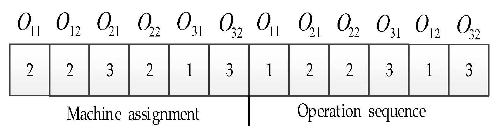
4.1. Encoding Mechanism

The low-carbon FJSP can be decomposed into two sub-problems: Machine selection and process sequencing. According to these characteristics, a two-segment coding method with equal lengths is used to represent it. Taking a FJSP with 3 jobs and 5 machines, for example, we assume that each job contains two operations. The scheduling solution is shown in Figure 1. In the first string, each element represents the selected machine number for each operation, which is stored in a fixed order. In the second string, each element equals the job code, where the elements represent different operations of the same job. In addition, $O_{ik}$ presents the k^th operation of the job i.

For each solution, the following procedure is adopted as the decoding method:

(1)

Read the operation sequence from left to right, and determine the machine number for each operation.

(2)

The first operation in the operation sequence string is processed first at the earliest available time on the assigned machine. The second operation is scheduled in the same way, and so on. Repetition of this procedure and a scheduling scheme can be achieved.

4.2. Population Initialization

In the first phase, the machine assignment is achieved by using a hybrid search method, in which 60% of the initial population is generated by the global search, 30% by a local search and 10% by a random search. Once the machine assignment is generated, the operation sequence should be generated in the second phase. For each machine assignment, a set of operation sequences are generated at random and combine with the machine assignment in turn. A combination of the two components which have the best fitness value is selected as an initial solution, and then the initial population can be obtained by repeating this procedure. The detailed description of the method can be found in [40].

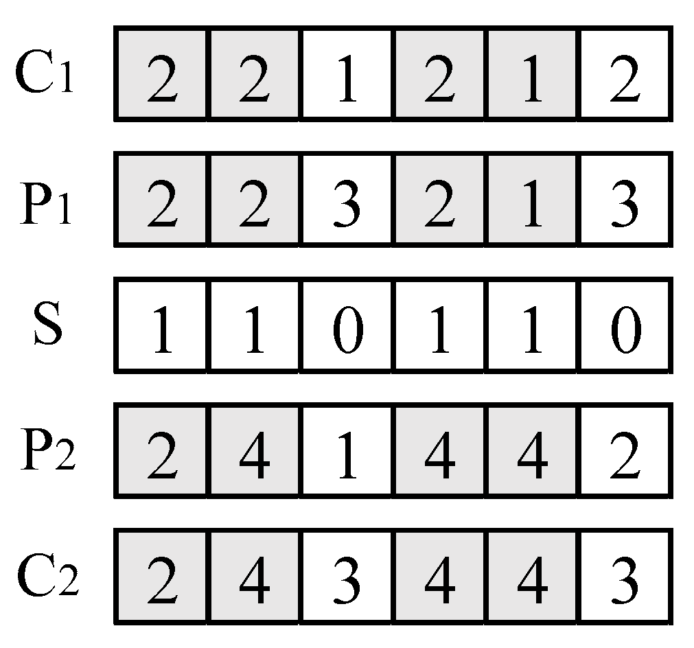
4.3. Discrete Encircling of the Prey

The original WOA was developed to solve continuous problems. However, as the low-carbon FJSP contains discrete characteristics, it means the original WOA cannot directly be applied to solve the problem. Therefore, some discrete individual updating methods were designed to make the WOA solve the problem directly.

In the encircling prey phase, individuals update their positions according to the information of the current optimal individuals. In our paper, the discrete individual updating approach based on the crossover operator $f_1$ is designed to replace the original update mode. If $h$ is smaller than 0.5, the crossover operator $f_1$ is executed between each individual and the current optimal individual, which is shown by Equation (18), where $h$ is a random number in the range [0,1]. In this study, the improved precedence preserving order-based crossover (IPOX) scheme is adopted for the operation sequence while the multi-point crossover (MPX) scheme is used for the machine assignment [41].

$$\mathit{X}(t+1)={\mathit{f}}_1\left(\mathit{X}\right(t), {\mathit{X}}^{\ast }(t\left)\right) \mathrm{if} h<0.5$$

(18)

The steps of the MPX scheme are described as follows, and illustrated in Figure 2.

Step 1. Randomly generate a 0–1 set $S$.

Step 2. Copy the machine number corresponding to the places with ‘1’ in set $S$ from $P_1$ to $C_1$ and from $P_2$ to $C_2$.

Step 3. Copy the rest machine numbers corresponding to the places with ‘0’ in set $S$ from $P_1$ to $C_2$ and from $P_2$ to $C_1$.

The steps of the IPOX scheme are described below and illustrated in Figure 3.

Step 1. Create two subsets $K_1$ and $K_2$.

Step 2. Copy some jobs into $K_1$, the rest of the jobs are copied into $K_2$.

Step 3. Choose the jobs in $K_1$ from $P_1$ to $C_1$ and ensure that their positions remain immobile; choose the jobs in $K_2$ from $P_2$ to $C_1$ and maintain their sequence.

Step 4. Choose the jobs in $K_2$ from $P_2$ to $C_2$ and maintain their positions; choose the jobs in K₁ from $P_1$ to $C_2$ and keep their sequence unchanged.

$$K_1=\left\{1\right\},K_2=\left\{2,3\right\}$$

4.4. Discrete Spiral Updating Mechanism

In the exploitation phase, the whale individuals update their positions in a helix shaped movement when encircling the prey. The other crossover operator $f_2$ is designed to replace the original spiral updating mechanism. If $h$ is bigger than 0.5, the crossover operator $f_2$ is executed between each individual and the current optimal individual, as shown in Equation (19). In this case, the random order-based crossover (ROX) scheme is employed for the operation sequence, and the two-point crossover (TPX) scheme is used for the machine assignment [42].

$$\mathit{X}(t+1)={\mathit{f}}_2\left(\mathit{X}\right(t), {\mathit{X}}^{\ast }(t\left)\right) \mathrm{if} h<0.5$$

(19)

The TPX scheme is illustrated in Figure 4 and described as follows.

Step 1. Choose two positions from parent individuals $P_1$ and $P_2$.

Step 2. Exchange the elements between the two chosen positions in $P_1$ and $P_2$ with each other to generate two children $C_1$ and $C_2$.

The steps of the ROX are represented by Figure 5 and illustrated as follows:

Step 1. Randomly generate two integers $i_1,i_2\in \left[1,\mathrm{n}\right]$, $n$ is the number of jobs.

Step 2. Copy the job with serial number $i_1$ from $P_1$ to $C_1$, and copy the rest of the jobs from $P_2$ to $C_1$ with their sequence unchanged.

Step 3. Copy the job with serial number $i_2$ from $P_2$ to $C_2$, and copy the rest of jobs from $P_1$ to $C_2$ with their sequence unchanged.

Step 4. Terminate the procedure.

$$i_2=1, i_1=2$$

4.5. Discrete Searching for the Prey

In the exploration phase, to search for the global optimum, we make the whale individual move far away from a reference whale by the random coefficient vector $A$, with its value less than −1 or greater than 1. At the same time, the whale individual updates their position by another whale individual randomly chosen from the population which defined by $X_{rand}(t)$, instead of the current optimal individual ${\overrightarrow{X}}^{\ast }(t)$, so that the WOA can perform a global search ability. In this paper, a discrete individual updating approach based on the crossover operator $f_3$ is designed in Equation (20) to replace the original update mode, where $X_{rand}(t)$ is a scheduling solution randomly chosen from the current population, and $f_3$ represents the crossover operation between the randomly chosen individual and other individuals. Here, $f_3$ executes the same operations associated with $f_1$ in Equation (18).

$$\mathit{X}(t+1)={\mathit{f}}_3\left(\mathit{X}\right(t), {\mathit{X}}_{rand}(t\left)\right)$$

(20)

4.6. Dynamic Adjustment Strategy of a

As mentioned above, transitions between exploration and exploitation mainly depend on the search vector $\mathit{A}$. By adjusting the value of $\mathit{A}$, some iterations are performed on exploration ($\left|\mathit{A}\right|\ge 1$), and the others are implemented on exploitation ($\left|\mathit{A}\right|<1$). According to Equation (10), the value of $\mathit{A}$ is dependent on the variation of $\mathit{a}$. However, $\mathit{a}$ linearly decreases over the course of iterations by Equation (13) in original WOA, which cannot effectively adjust the transition between exploration and exploitation. Therefore, a sequence of adjustment curves of a is employed, by which whales can explore the optimum in a large space at the early stage of iterations, and exploit the local optimum to gain the global optimum at the latter stage. To execute it, six dynamic adjustment curves of $\mathit{a}$ are adopted in Equations (21)–(26), where ${\mathit{a}}_{\min }$ and ${\mathit{a}}_{\max }$ are the minimum and maximum values of $\mathit{a}$, $t_{\max }$ is the maximum iteration. The corresponding algorithms are named as LDWOA, SinDWOA, CosDWOA, TanDWOA, LnDWOA and SquareDWOA.

$$a=a_{\max }-(a_{\max }-a_{\min })t/t_{\max }$$

(21)

$$a=a_{\max }-(a_{\max }-a_{\min })\sin (t\pi /2t_{\max })$$

(22)

$$a=a_{\max }-(a_{\max }-a_{\min })\cos (t\pi /2t_{\max })$$

(23)

$$a=a_{\max }-(a_{\max }-a_{\min })\tan (t\pi /2t_{\max })$$

(24)

$$a=a_{\max }-(a_{\max }-a_{\min })\ln (1+t(e-1)/t_{\max })$$

(25)

$$a=a_{\max }-(a_{\max }-a_{\min }){(t/t_{\max })}^2$$

(26)

4.7. Variable Neighborhood Search

In the local exploration phase, the whale individuals update their positions toward the current optimal solution $X^{\ast }$. Therefore, $X^{\ast }$ determines the accuracy of the local exploration to some extent. To gain the global optimal solution with high quality, a variable neighborhood search (VNS) strategy is introduced into the algorithm to improve the quality of the current optimal scheduling solution $X^{\ast }$, which executes on the current optimal solution in each iteration and terminates after the fixed number of iterations. At the same time, an “iterative counter” with the value of 0 at the time zero is set for $X^{\ast }$. If $X^{\ast }$ remains unchanged, the value of “iterative counter” increases by 1, otherwise, it remains the same. When the value of the “iterative counter” is equal to 10, as the individuals reach the steady state, the variable neighborhood search operation is executed on $X^{\ast }$, which makes $X^{\ast }$ escape from the local optimum.

In the VNS, three types of neighborhood structures are employed as follows.

The neighborhood structure $N_1$. Two random positions with different jobs in the second segment are chosen, then insert the job of the first random position in the position behind the second random position.

The neighborhood structure $N_2$. Randomly choose two positions, and then exchange the order of the elements of the two selected positions.

The neighborhood structure $N_3$. An operation which has more than one alternative machine is randomly selected in the first segment. Then, a machine with the shortest processing time in alternative machines is selected to replace the original one.

Based on the above neighborhood structures, the steps of the VNS are described in detail in the following.

Step 1. Set $X^{\prime }\leftarrow X^{\ast }$, $\phi >0$, $\mu =1$, $\kappa =1$ and maximum iteration ${\mu }_{\max }$.

Step 2. If $\kappa =1$, then $X^{″}\leftarrow N_1(X^{\prime })\cup N_3(X^{\prime })$; else if $\kappa =0$, then $X^{″}\leftarrow N_2(X^{\prime })\cup N_3(X^{\prime })$. Here, $N_1(X^{\prime })\cup N_3(X^{\prime })$ represents the execution of the operations of the neighborhood structure $N_1$ and $N_3$ on $X^{\prime }$, simultaneously.

Step 3. If $F(X^{″})-F(X^{\prime })\le \phi$, then $X^{\prime }\leftarrow X^{″}$; otherwise, κ←|κ − 1|.

Step 4. Set $\mu \leftarrow \mu +1$, if $\mu >{\mu }_{\max }$, then $X^{\prime }\leftarrow X^{″}$, go to Step 5; otherwise, go to Step 2.

Step 5. End and output $X^{\prime }$.

4.8. Procedure of Discrete Whale Optimization Algorithm

The detailed steps of the proposed DWOA are described below.

Step 1. Set parameters and generate the initial population by utilizing a hybrid search method.

Step 2. Evaluate the fitness value of each individual, and then find out the current optimal individual.

Step 3. Judge whether the value of the “iterative counter” is equal to 10. If yes, go to Step 4; otherwise, go to Step 5.

Step 4. Execute the local search operation on $X^{\ast }$ in VNS, and update $X^{\ast }$.

Step 5. Execute the individual updating procedure below for each individual.

Step 6. Check whether the maximum iteration is met. If yes, go to Step 7; otherwise, set $t=t+1$, go to Step 2.

Step 7. When the algorithm terminates save the final output $X^{\ast }$.

5. Computational Experiment

5.1. Experimental Settings

To evaluate the performance of the proposed DWOA, the algorithm was coded in Matlab 2016b and run on a computer configured with an Intel Core i5-8250 central processing unit (CPU) with 1.80 GHz frequency, 8 GB random access memory (RAM), and a Windows 10 operating system. We established the instances based on the well-known benchmark flexible job shop instances MK01–MK10 from Brandimarte [43], KA01–KA05 from Kacem et al. [44] and five random instances (RM01–RM05). The processing cost per unit time of all operations on any machine was 50. In the benchmark instances, the energy consumption cost per unit time of machine for processing all jobs was generated at random in (0,1), and the energy consumption cost per unit time of machine on the standby mode was also generated at random in (0,1). Of the random instances, five instances were generated in terms of the number of machines and the number of jobs. The processing times of operations were generated randomly following a discrete uniform distribution in (0,100), and the processing sequence of each job was also generated at random. In addition, the energy consumption cost per unit time of machines for processing all jobs and the energy consumption cost per unit time of the machines on the standby mode was also generated at random in (0,1).

5.2. Effectiveness of Dynamic Adjustment of the Parameter a

We first compared the performance of the six algorithms with different adjustment curves of $a$ in Figure 6, Figure 7, Figure 8 and Figure 9. Parameters of the algorithms were set as follows: The population size was 50, the maximum iteration $t_{\max }$ was 500, the maximum iteration of variable neighborhood search and local search were 10 and 20, respectively. For each algorithm, ten independent runs were executed for each instance. In Figure 6, ‘Avg’ defines the average values of the ten runs. In Figure 7, ‘Best’ means the best value obtained in the ten runs.In Figure 8, ‘Time’ is the average computation time (in seconds). In Figure 9, ‘ARPD’ denotes the average relative percent difference, as shown in Equation (27), where ‘R’ is the number of runs. ‘Min’ is the minimum solution in the ten runs. ‘$Ao{l}_r$’ is the obtained value in the r^th run by the algorithm for each instance. ‘Mean’ denotes the average results obtained by each algorithm for the nineteen instances.

For the ‘Best’ value, CosDWOA obtained 16 optimal values out of 19 instances. The second best algorithms, LDWOA and LnDWOA, obtained two optimal values. In addition, CosDWOA obtained the optimal mean value compared to the other algorithms.

For the ‘Avg’ value, CosDWOA obtained nine optimal values out of 19 instances. The second best algorithm, SquareDWOA, obtained three optimal values. The next best algorithms, SinDWOA, LnDWOA and TanDWOA obtained two optimal values. In addition, LnDWOA obtained a better mean value compared to those of the other algorithms.

For the ‘ARPD’ value, LDWOA obtained six optimal values out of 19 instances. The second best algorithm, CosDWOA, obtained five optimal values. The third best algorithm, SquareDWOA, obtained 4 optimal values. In addition, LDWOA obtained a better mean value than the mean values of the other algorithms.

For the ‘Time’ value, LnDWOA obtained 14 optimal values out of 19 instances. The second best algorithm, TanDWOA, obtained 13 optimal values. The third best algorithm, SinDWOA, obtained 10 optimal values. In addition, LnDWOA obtained the optimal mean value compared to the mean values of the other algorithms.

From the above, we can see that CosDWOA obtained the most optimal solution in a relative reasonable time.

$$ARPD={\displaystyle \sum _{r=1}^R\frac{100\times (Ao{l}_r-Min)}{Min}/R}$$

(27)

To analyze the results in Figure 6, Figure 7, Figure 8 and Figure 9 using a statistical method, a statistical result obtained by an analysis of variance (ANOVA) test is shown in

Table 1. ANOVA table for ARPD of six different DWOAs.

Source	DF	SS	MS	F	p-Value
Factor	4	17.99411	4.49853	0.67969	0.60748
Error	109	721.41302	6.61847
Total	113	739.40713

, where ARPD is considered as the response variable and each algorithm is viewed as a factor.‘DF’ is the degree of freedom. ’SS’ means the sum of squares. ‘MS’ represents mean square. ‘F’ is F-ratio. ‘p-Value’ is the presumed value The statistical results show that the p-value obtained is very close to zero, which means there is an obvious distinction between the algorithms.

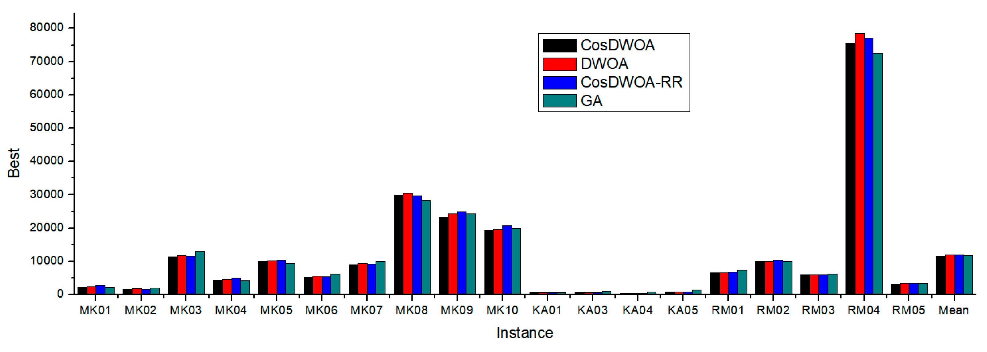
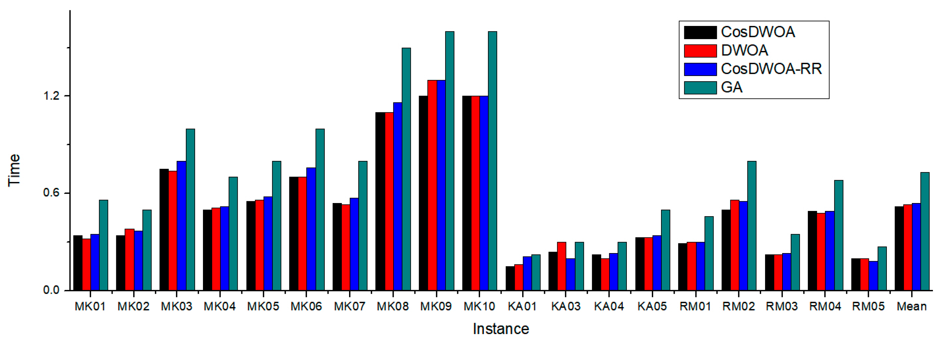
5.3. Effectiveness Analysis of Improvement Strategies

In this study, some improvement strategies are implemented to improve the performance of the proposed DWOA. The hybrid search method is applied to improve the quality of the initial population, and a dynamic adjustment strategy for $\mathit{a}$ is employed to adjust the transition between exploration and exploitation. As shown in Figure 10, Figure 11, Figure 12 and Figure 13, the effectiveness of two improvement strategies are tested, where ‘DWOA’ represents the algorithm where nonlinear convergence factor $\mathit{a}$ of CosDWOA is replaced by the original Equation (12). ‘CosDWOA-RR’ presents the algorithm where the initial populations are generated at random. ‘GA’ presents the original genetic algorithm.

For the ‘Best’ value, CosDWOA obtained 16 optimal values out of 19 instances. For the ‘Avg’ value, CosDWOA obtained 10 optimal values out of 19 instances. For the ‘ARPD’ value, DWOA and CosDWOA-RR obtained seven optimal values out of 19 instances. For the ‘Time’ value, CosDWOA and DWOA obtained 11 optimal values out of 19 instances. The effectiveness analysis demonstrated that CosDWOA was able to obtain the most satisfactory solution in a reasonable time.

To analyze the results in Figure 10, Figure 11, Figure 12 and Figure 13 in a statistical method, a statistical result obtained by an analysis of variance (ANOVA) test is shown in

Table 2. ANOVA table for ARPD of five compared algorithms.

Source	DF	SS	MS	F	p-Value
Factor	2	1175.80737	587.90368	13.31722	1.17311 × 10−5
Error	73	3222.66733	44.14613	-	-
Total	75	4398.47469	-	-	-

, where ARPD is considered as the response variable and each algorithm is viewed as a factor. The statistical results show that the p-value obtained is very close to zero, which means there is an obvious distinction between the algorithms.

6. Conclusions

In this paper, an extended whale optimization algorithm (DWOA) is developed to solve the low-carbon FJSP with the objective of minimizing the sum of energy consumption cost and processing cost.

The job shop scheduling problems and its variants still receive abundant attention in the literature, as they are being implemented into many real-life applications such as in food, chemical, automation, railway, robotics, aviation, healthcare and mining industries [45,46,47,48,49,50,51,52,53,54]. In this framework, a two-component encoding method was designed to represent the problem, and a hybrid search method was employed to generate the initial population with high quality and diversity. By considering the discrete characteristics of the problem, the modified updating approaches based on the crossover operator were proposed to replace the original updating method in the exploration and exploitation phase, by which the WOA can work directly in a discrete domain. In addition, in order to balance the ability of exploration and exploitation in the process of evolution, six adjustment curves were used to adjust the transition between exploration and exploitation. Extensive experiments based on benchmark instances and randomly generated instances were executed. Computational results demonstrated that among the proposed six DWOA algorithms associated with different adjustment curves, the CosDWOA obtained the best result within a reasonable computational time. It is verified that the hybrid variable neighborhood search based on a population initialization method and an adjustment mechanism is effective for improving the optimality performance of the proposed DWOA.

Regarding future work, the low-carbon FJSP should be further studied by considering some practical constraints, e.g., adjustable speeds of machines, machine breakdown, arrival of new jobs, blocking and no-wait constraints [55,56,57]. For the DWOA, some effective neighborhood structures for the low-carbon FJSP should be designed to further improve the quality of the optimal solution. Finally, it would be a promising research direction to apply the DWOA to solve other combinatorial optimization problems.

References

1. Dai, M.; Tang, D.; Giret, A.; Salido, M.A.; Li, W.D. Energy efficient scheduling for a flexible flowshop using an improved genetic-simulated annealing algorithm. Robot. Comput. Int. Manuf. 2013, 29, 418–429. [Google Scholar] [CrossRef]
2. Ding, J.Y.; Song, S.; Wu, C. Carbon-efficient scheduling of flow shops by multi-objective optimization. Eur. J. Oper. Res. 2016, 248, 758–771. [Google Scholar] [CrossRef]
3. Mansouri, S.A.; Aktas, E.; Besikci, U. Green scheduling of a two-machine flowshop: Trade-off between makespan and energy consumption. Eur. J. Oper. Res. 2016, 248, 772–788. [Google Scholar] [CrossRef] [Green Version]
4. Luo, H.; Du, B.; Huang, G.Q.; Chen, H.; Li, X. Hybrid flow shop scheduling considering machine electricity consumption cost. Int. J. Prod. Econ. 2013, 146, 423–439. [Google Scholar] [CrossRef]
5. Zhang, R.; Chiong, R. Solving the energy-efficient job shop scheduling problem: A multi-objective genetic algorithm with enhanced local search for minimizing the total weighted tardiness and total energy consumption. J. Clean. Prod. 2016, 112, 3361–3375. [Google Scholar] [CrossRef]
6. Liu, G.S.; Zhang, B.X.; Yang, H.D.; Chen, X.; Huang, G.Q. A branch-and-bound algorithm for minimizing the energy consumption in the PFS problem. Math. Probl. Eng. 2013, 2013, 546810. [Google Scholar] [CrossRef]
7. Li, J.Q.; Sang, H.Y.; Han, Y.Y.; Wang, C.G.; Gao, K.Z. Efficient multi-objective optimization algorithm for hybrid flow shop scheduling problems with setup energy consumptions. J. Clean. Prod. 2018, 181, 584–598. [Google Scholar] [CrossRef]
8. Salido, M.A.; Escamilla, J.; Giret, A.; Barber, F. A genetic algorithm for energy-efficiency in job-shop scheduling. Int. J. Adv. Manuf. Technol. 2016, 85, 1303–1314. [Google Scholar] [CrossRef]
9. Brucker, P.; Schlie, R. Job-shop scheduling with multi-purpose machines. Computing 1990, 45, 369–375. [Google Scholar] [CrossRef]
10. Kaskavelis, C.A.; Caramanis, M.C. Efficient Lagrangian relaxation algorithms for industry size job-shop scheduling problems. IIE Trans. 1998, 30, 1085–1097. [Google Scholar] [CrossRef]
11. Chen, H.; Chu, C.; Proth, J.M. An improvement of the Lagrangian relaxation approach for job shop scheduling: A dynamic programming method. IEEE Trans. Robot Autom. 1998, 14, 786–795. [Google Scholar] [CrossRef]
12. Ríos-Mercado, R.Z.; Bard, J.F. Computational experience with a branch-and-cut algorithm for flowshop scheduling with setups. Comput. Oper. Res. 1998, 25, 351–366. [Google Scholar] [CrossRef]
13. Karimi-Nasab, M.; Modarres, M. Lot sizing and job shop scheduling with compressible process times: A cut and branch approach. Comput. Ind. Eng. 2015, 85, 196–205. [Google Scholar] [CrossRef]
14. Dauzere-Peres, S.; Paulli, J. An integrated approach for modeling and solving the general multi-processor job-shop scheduling problem using tabu search. Ann. Oper. Res. 1997, 70, 281–306. [Google Scholar] [CrossRef]
15. Li, J.Q.; Pan, Q.K.; Suganthan, P.N. A hybrid tabu search algorithm with an efficient neighborhood structure for the flexible job shop scheduling problem. Int. J. Adv. Manuf. Technol. 2011, 52, 683–697. [Google Scholar] [CrossRef]
16. Wang, L.; Zhou, G.; Xu, Y.; Wang, S.; Liu, M. An effective artificial bee colony algorithm for the flexible job-shop scheduling problem. Int. J. Adv. Manuf. Technol. 2012, 60, 303–315. [Google Scholar] [CrossRef]
17. Liouane, N.; Saad, I.; Hammadi, S.; Borne, P. Ant systems and local search optimization for flexible job shop scheduling production. Int. J. Comput. Commun. Control 2007, 2, 174–184. [Google Scholar] [CrossRef]
18. Yuan, Y.; Xu, H.; Yang, J.D. A hybrid harmony search algorithm for the flexible job shop scheduling problem. Appl. Soft. Comput. 2013, 13, 3259–3272. [Google Scholar] [CrossRef]
19. Li, X.; Gao, L. An effective hybrid genetic algorithm and tabu search for flexible job shop scheduling problem. Int. J. Prod. Econ. 2016, 174, 93–110. [Google Scholar] [CrossRef]
20. Yin, L.; Li, X.; Gao, L.; Lu, C.; Zhang, Z. A novel mathematical model and multi-objective method for the low-carbon flexible job shop scheduling problem. Sustain. Comput. Inform. 2017, 13, 15–30. [Google Scholar] [CrossRef]
21. Xiong, W.; Fu, D. A new immune multi-agent system for the flexible job shop scheduling problem. J. Intell. Manuf. 2018, 29, 857–873. [Google Scholar] [CrossRef]
22. Piroozfard, H.; Wong, K.Y.; Wong, W.P. Minimizing total carbon footprint and total late work criterion in flexible job shop scheduling by using an improved multi-objective genetic algorithm. Resour. Conserv. Recycl. 2018, 128, 267–283. [Google Scholar] [CrossRef]
23. Mokhtari, H.; Hasani, A. An energy-efficient multi-objective optimization for flexible job-shop scheduling problem. Comput. Chem. Eng. 2017, 104, 339–352. [Google Scholar] [CrossRef]
24. Shen, L.; Dauzère-Pérès, S.; Neufeld, J.S. Solving the flexible job shop scheduling problem with sequence-dependent setup times. Eur. J. Oper. Res. 2018, 265, 503–516. [Google Scholar] [CrossRef]
25. Zandieh, M.; Khatami, A.R.; Rahmati, S.H.A. Flexible job shop scheduling under condition-based maintenance: Improved version of imperialist competitive algorithm. Appl. Soft. Comput. 2017, 58, 449–464. [Google Scholar] [CrossRef]
26. Nouiri, M.; Bekrar, A.; Jemai, A.; Niar, S.; Ammari, A.C. An effective and distributed particle swarm optimization algorithm for flexible job-shop scheduling problem. J. Intell. Manuf. 2018, 29, 603–615. [Google Scholar] [CrossRef]
27. Wu, X.; Wu, S. An elitist quantum-inspired evolutionary algorithm for the flexible job-shop scheduling problem. J. Intell. Manuf. 2017, 28, 1441–1457. [Google Scholar] [CrossRef]
28. Jiang, T.H.; Deng, G.L. Optimizing the low-carbon flexible job shop scheduling problem considering energy consumption. IEEE Access. 2018, 6, 46346–46355. [Google Scholar] [CrossRef]
29. Jiang, T.H.; Zhang, C. Application of grey wolf optimization for solving combinatorial problems: Job shop and flexible job shop scheduling cases. IEEE Access. 2018, 6, 26231–26240. [Google Scholar] [CrossRef]
30. Jiang, T.H.; Zhang, C.; Sun, Q. Green job shop scheduling problem with discrete whale optimization algorithm. IEEE Access. 2019, 7, 43153–43166 . [Google Scholar] [CrossRef]
31. Sharma, N.; Sharma, H. Beer froth artificial bee colony algorithm for job shop scheduling problem. Appl. Soft. Comput. 2018, 68, 507–524. [Google Scholar] [CrossRef]
32. Mirjalili, S.; Lewis, A. The Whale Optimization Algorithm. Adv. Eng. Soft. 2016, 95, 51–67. [Google Scholar] [CrossRef]
33. Medani, K.B.O.; Sayah, S.; Bekrar, A. Whale optimization algorithm based optimal reactive pow-er dispatch: A case study of the Algerian power system. Electr. Power Syst. Res. 2018, 163, 696–705. [Google Scholar] [CrossRef]
34. Mafarja, M.M.; Mirjalili, S. Hybrid Whale Optimization Algorithm with simulated annealing for feature selection. Neurocomputing 2017, 260, 302–312. [Google Scholar] [CrossRef]
35. Aziz, M.A.E.; Ewees, A.A.; Hassanien, A.E. Whale Optimization Algorithm and Moth-Flame Optimization for multilevel thresholding image segmentation. Expert Syst. Appl. 2017, 83, 242–256. [Google Scholar] [CrossRef]
36. Oliva, D.; Aziz, M.A.E.; Hassanien, A.E. Parameter estimation of photovoltaic cells using an improved chaotic whale optimization algorithm. Appl. Energy 2017, 200, 141–154. [Google Scholar] [CrossRef]
37. Jiang, T.H.; Zhang, C.; Zhu, H.Q.; Zhu, H.Q.; Gu, J.C.; Deng, G.L. Energy-efficient scheduling for a job shop using an improved whale optimization algorithm. Mathematics 2018, 6, 220. [Google Scholar] [CrossRef]
38. Abdel-Basset, M.; El-Shahat, D.; Sangaiah, A.K. A modified nature inspired meta-heuristic whale optimization algorithm for solving 0–1 knapsack problem. Int. J. Mach. Learn. Cybern. 2019, 10, 495–514. [Google Scholar] [CrossRef]
39. Abdel-Basset, M.; Manogaran, G.; El-Shahat, D.; Mirjalili, S. A hybrid whale optimization algorithm based on local search strategy for the permutation flow shop scheduling problem. Future Gener. Comp. Syst. 2018, 85, 129–145. [Google Scholar] [CrossRef]
40. Zhang, G.H.; Gao, L.; Li, P.G.; Zhang, C.Y. Improved genetic algorithm for the flexible job shop scheduling problem. J. Mech. Eng. 2009, 45, 145–151. (In Chinese) [Google Scholar] [CrossRef]
41. Zhang, C.Y.; Dong, X.; Wang, X.J.; Li, X.Y.; Liu, Q. Improved NSGA-II for the multi-objective flexible job-shop scheduling problem. J. Mech. Eng. 2010, 46, 156–164. (In Chinese) [Google Scholar] [CrossRef]
42. Wang, L.; Cai, J.C.; Shi, X. Multi-objective flexible job shop energy-saving scheduling problem based on improved genetic algorithm. J. Nanjing Univ. Sci. Technol. Nat. Sci. 2017, 41, 494–502. (In Chinese) [Google Scholar]
43. Brandimarte, P. Routing and scheduling in a flexible job shop by tabu search. Ann. Oper. Res. 1993, 41, 157–183. [Google Scholar] [CrossRef]
44. Kacem, I.; Hammadi, S.; Borne, P. Approach by localization and multiobjective evolutionary optimization for flexible job-shop scheduling problems. IEEE. Trans. Syst. Man Cyber. Part C Appl. Rev. 2002, 32, 1–13. [Google Scholar] [CrossRef]
45. Kozan, E.; Liu, S.Q. An Operational-Level Multi-Stage Mine Production Timetabling Model for Optimally Synchronising Drilling, Blasting and Excavating Operations. Int. J. Min. Reclam. Environ. 2017, 31, 457–474. [Google Scholar] [CrossRef]
46. Liu, S.Q.; Kozan, E. Scheduling trains as a blocking parallel-machine job shop scheduling problem. Comput. Oper. Res. 2009, 36, 2840–2852. [Google Scholar] [CrossRef] [Green Version]
47. Liu, S.Q.; Kozan, E. Scheduling trains with priorities: A no-wait blocking parallel-machine job-shop scheduling model. Transp. Sci. 2011, 45, 175–198. [Google Scholar] [CrossRef]
48. Liu, S.Q.; Kozan, E. A hybrid shifting bottleneck procedure algorithm for the parallel-machine job-shop scheduling problem. J. Oper. Res. Soc. 2012, 63, 168–182. [Google Scholar] [CrossRef]
49. Liu, S.Q.; Kozan, E. A hybrid metaheuristic algorithm to optimise a real-world robotic cell. Comput. Oper. Res. 2017, 84, 188–194. [Google Scholar] [CrossRef]
50. Masoud, M.; Kozan, E.; Kent, G.; Liu, S.Q. An integrated approach to optimise sugarcane rail operations. Comput. Ind. Eng. 2016, 98, 211–220. [Google Scholar] [CrossRef] [Green Version]
51. Masoud, M.; Kozan, E.; Kent, G.; Liu, S.Q. A new constraint programming approach for optimising a coal rail system. Optim. Lett. 2017, 11, 725–738. [Google Scholar] [CrossRef]
52. Mousavi, A.; Kozan, E.; Liu, S.Q. Open-pit block sequencing optimization: A mathematical model and solution technique. Eng. Optim. 2016, 48, 1932–1950. [Google Scholar] [CrossRef]
53. Yan, P.; Che, A.; Levner, E.; Liu, S.Q. A heuristic for inserting randomly arriving jobs into an existing hoist schedule. IEEE Trans. Autom. Sci. Eng. 2017, 15, 1423–1430. [Google Scholar] [CrossRef]
54. Yan, P.; Liu, S.Q.; Sun, T.; Ma, K. A dynamic scheduling approach for optimizing the material handling operations in a robotic cell. Comput. Oper. Res. 2018, 99, 166–177. [Google Scholar] [CrossRef]
55. Liu, S.Q.; Kozan, E. Parallel-identical-machine job-shop scheduling with different stage-dependent buffering requirements. Comput. Oper. Res. 2016, 74, 31–41. [Google Scholar] [CrossRef]
56. Liu, S.Q.; Kozan, E.; Masoud, M.; Zhang, Y.; Chan, F.T.S. Job shop scheduling with a combination of four buffering constraints. Int. J. Prod. Res. 2018, 56, 3274–3293. [Google Scholar] [CrossRef]
57. Yan, P.; Liu, S.Q.; Yang, C.; Masoud, M. A comparative study on three graph-based constructive algorithms for multi-stage scheduling with blocking. J. Ind. Manag. Optim. 2019, 15, 221–233. [Google Scholar] [CrossRef] [Green Version]
Figure 1. Two-string encoding method.
Mathematics 07 00688 g001
Figure 2. Multi-point crossover (MPX) scheme.
Mathematics 07 00688 g002
Figure 3. IPOX crossover operation.
Mathematics 07 00688 g003
Figure 4. Two-point crossover (TPX) operation.
Mathematics 07 00688 g004
Figure 5. ROX crossover operation.
Mathematics 07 00688 g005
Figure 6. Average values of the six dynamic adjustment strategy.
Mathematics 07 00688 g006
Figure 7. Best values of the six dynamic adjustment strategy.
Mathematics 07 00688 g007
Figure 8. ARPD value of the six dynamic adjustment strategy.
Mathematics 07 00688 g008
Figure 9. Time value of the six dynamic adjustment strategy.
Mathematics 07 00688 g009
Figure 10. Average values of the four compared algorithms.
Mathematics 07 00688 g010
Figure 11. Best values of the four compared algorithms.
Mathematics 07 00688 g011
Figure 12. ARPD value of the four compared algorithms.
Mathematics 07 00688 g012
Figure 13. Time value of the four compared algorithms.
Mathematics 07 00688 g013