Practical Stability with Respect to h-Manifolds for Impulsive Control Functional Differential Equations with Variable Impulsive Perturbations

Abstract

The present paper is devoted to the problems of practical stability with respect to h-manifolds for impulsive control differential equations with variable impulsive perturbations. We will consider these problems in light of the Lyapunov–Razumikhin method of piecewise continuous functions. The new results are applied to an impulsive control cellular neural network model with variable impulsive perturbations.

1. Introduction

Impulsive control problems are well described by impulsive differential systems. Due to their numerous applications in various fields, such as engineering [1,2,3], biotechnologies and ecosystems management [4], chemical kinetics [5], and finance and investment [6,7], such systems have been extensively studied in past years. See, for example, [8,9] and the references therein for some fundamental results on impulsive differential equations and related impulsive control models. Indeed, due to numerous factors of an internal and external nature, the behavior of a real-world problem can often be affected by momentary changes at certain instants. Economic shocks are typical examples of sudden disturbances in a real-world system. Furthermore, some perturbations in impulsive biological models that are caused by nature or man can be used for control purposes. In addition, the importance of electronic impulse control with all its variations compared to conventional mechanical versions is growing constantly. The paper of Yang et al. [10] offered a comprehensive overview of the recent progress in impulsive control systems. Practical applications have now verified the theoretical advantages of the impulsive control strategy by demonstrating its superior efficiency to allow synchronization of a complex system by using only small control impulses, to lower the communication cost and enhance the security of chaotic systems.

On the other hand, in the real world, impulsive control systems contain some information about their past states. The potential role of the memory in impulsive control systems has been explored in various contexts, and hence, applied impulsive control systems with delays have received considerable attention from many authors [11,12,13,14,15,16].

Stability in the sense of Lyapunov has been a main focus of intensive study in impulsive control models. However, in many applications of impulsive models, some extensions of the stability notion are more appropriate. In the proposed research, we will further expand our studies on the stability behavior of the states with a particular focus on the so-called practical stability [17]. It is well known that the key issue in the practical stability notion is in investigating sets close to a particular state knowing its initial data domain, as well as the domain in which the state must belong. It is possible that the study state is unstable in the sense of Lyapunov; however a solution of the system can oscillate sufficiently close to the investigated state so as to consider its behavior as an acceptable one. In some cases, although a system is stable or asymptotically stable in the Lyapunov sense, it is actually useless from the engineering point of view because the behavioral characteristics are not desirable; for example, because the stability domain or the attraction domain is not large enough. Therefore, practical stability and stabilization are of a significant importance in scientific and practical engineering problems [18,19].

The practical stability notion has also important theoretical value and practical importance to impulsive control systems, and some practical stability results for such systems have already been reported in the literature; see [20,21,22,23,24,25]. However, in order to establish practical stability or synchronization criteria, all above-cited papers investigated impulsive control effects at fixed instants. The problem of the practical stability of impulsive control systems with variable impulsive perturbations is not yet fully developed, and this is the main aim of our paper. Indeed, considering impulsive perturbations in variable times is more general from theoretical and applied points of view, and such impulsive systems have important applications. See, for example, [26,27,28] and the references therein.

In addition, in this paper, we study the stability of a manifold defined by a specific function. Because of the great possibilities for applications, the topic of stable manifolds whether or not related to equilibrium states has been studied for different classes of differential equations [29,30,31,32], but the concept has not been well applied to the practical stability of impulsive systems [33].

It is worth pointing out that variable impulsive perturbations were considered for impulsive systems only in [34]. In the present paper, compared with all previous works, we study variable impulsive perturbations, as well as h-manifolds in our practical stability analysis. The unique features of our results can be distinguished in the following aspects.

1. The important notion of practical stability is extended to the case of h-manifolds, which generalizes the stability concept, and includes numerous particular cases. In most of the impulsive functional differential systems in the available literature, the concepts of practical stability and stability with respect to manifolds are not taken into consideration simultaneously. This shows the novelty of our proposed result.

The first motivation for considering such extensions of stability is to develop a rigorous stability theory that will be of a great importance for researchers of impulsive differential systems with variable impulsive perturbations. The second motivation comes from the applicable point of view, since the extended stability notions for systems with not fixed moments of impulsive perturbations have significant practical applications in emerging areas such as optimal control, biology, mechanics, medicine, bio-technologies, electronics, economics, etc.

2. The combined dynamic effects of variable impulsive perturbations and functional differential terms on the extended stability properties of the system under consideration are investigated in the proposed criteria.

3. The feasibility of the new obtained results is demonstrated by using a class of neural network systems that have numerous applications in science and technologies.

The remaining part of the paper is organized as follows. In Section 2, we introduce some notations and preliminaries. Some notions related to practical stability introduced in [17] are generalized. In Section 3, sufficient conditions are obtained that guarantee the practical stability of a manifold with respect to an impulsive control delayed system with variable impulsive perturbations. In Section 4, to show the effectiveness of the obtained results, we apply the obtained criteria to an impulsive neural network model. Finally, some concluding remarks are drawn in Section 5.

2. Preliminaries

Let ${\mathbb{R}}^n$ be the n-dimensional Euclidean space with norm $\left|\right|.\left|\right|$, $\mathsf{\Omega }$ be an open set in ${\mathbb{R}}^n$ containing the origin, and ${\mathbb{R}}_{+}=[0,\infty )$.

Let $t_0\in {\mathbb{R}}_{+}$, $J\subset {\mathbb{R}}_{+}$ be an interval. Define the following classes of functions:

$PC[J,{\mathbb{R}}^n]=\left\{\sigma :J\to {\mathbb{R}}^n:\sigma \left(t\right)\right.$ is continuous everywhere except at some points $t_k\in J$ at which $\sigma \left(t_k^{-}\right)$ and $\sigma \left(t_k^{+}\right)$ exist and $\sigma \left(t_k^{-}\right)=\sigma \left(t_k\right)\}$;

$\mathcal{PC}=PC\left[\right[-\nu ,0],\mathsf{\Omega }]$, $\nu =const>0$.

Let $f:[t_0,\infty )\times \mathcal{PC}\to {\mathbb{R}}^n$, ${\tau }_k:\mathsf{\Omega }\to {\mathbb{R}}_{+}$, $I_k:\mathsf{\Omega }\to {\mathbb{R}}^n,k=1,2,\dots$

In this research, we will consider a nonlinear impulsive control delayed system with variable impulsive perturbations. A system of this class is written as follows:

$$\left\{\begin{array}{c}\dot{x}\left(t\right)=f(t,x_t)),t\ne {\tau }_k\left(x\left(t\right)\right),\hfill \\ \Delta x\left(t\right)=I_k\left(x\left(t\right)\right),t={\tau }_k\left(x\left(t\right)\right),k=1,2,\dots ,\hfill \end{array}\right.$$

(1)

where $x_t\in \mathcal{PC}$ and $\Delta x\left(t\right)=x\left(t^{+}\right)-x\left(t\right)$, $t>t_0$.

The second part of the impulsive system (1) is the control or jump condition. The functions $I_k$ that determine the controlled outputs $x\left(t^{+}\right)$ are the impulsive functions. In impulsive control systems of Type (1), these functions are considered as control forces. For the basic concepts and theorems of such systems, we refer the reader to [8,9,26,27].

Let ${\phi }_0\in PCB[[-\nu ,0],\mathsf{\Omega }]$, where $PCB[J,\mathsf{\Omega }]=\{\sigma \in PC[J,\mathsf{\Omega }]:\sigma (t)$ is bounded on J}.

Denote by $x\left(t\right)=x(t;t_0,{\phi }_0),x\in {\mathbb{R}}^n$ the solution of System (1) that satisfies the initial conditions:

$$\left\{\begin{array}{c}x(t;t_0,{\phi }_0)={\phi }_0(t-t_0),t_0-\nu \le t\le t_0,\hfill \\ x(t_0^{+};t_0,{\phi }_0)={\phi }_0\left(0\right).\hfill \end{array}\right.$$

(2)

The solution $x\left(t\right)=x(t;t_0,{\phi }_0)={(x_1(t;t_0,{\phi }_0),\dots ,x_n(t;t_0,{\phi }_0))}^T$ of the Initial Value Problem (IVP) (1), (2) is [8,9,26] a piecewise continuous function with points of discontinuity of the first kind at which it is left continuous; i.e., at the moments $t_{l_k}$ when the integral curve of the solution $x\left(t\right)$ meets the hypersurfaces:

$${\sigma }_k=\left\{(t,x)\in [t_0,\infty )\times \mathsf{\Omega }:t={\tau }_k\left(x\right)\right\},$$

and where it is continuous from the left, the following relations are satisfied:

$$x\left(t_{l_k}^{-}\right)=x\left(t_{l_k}\right),x\left(t_{l_k}^{+}\right)=x\left(t_{l_k}\right)+I_{l_k}\left(x\left(t_{l_k}\right)\right).$$

The points $t_{l_1},t_{l_2},\dots$ ($t_0<t_{l_1}<t_{l_2}<\dots$) are the impulsive control instants. Let us note that, in general, $k\ne l_k$.

In this paper, we will investigate such trajectories of solutions $x\left(t\right)$, the motion along which must be ensured by an appropriate choice of impulsive forces. That is why we suppose that the functions $f,I_k$, and ${\tau }_k\left(x\right),k=1,2,\dots$ are smooth enough on their domains to guarantee the absence of the phenomenon of the “beating” of the solutions, existence, uniqueness, and continuability of the solution $x\left(t\right)=x(t;t_0,{\phi }_0)$ of (IVP) (1), (2) on the interval $[t_0,\infty )$ for any $t_0\in {\mathbb{R}}_{+}$ and ${\phi }_0\in PCB[[-\nu ,0],\mathsf{\Omega }]$ [8,9,26,27].

Let $h=h(t,x),h:[t_0-\nu ,\infty )\times \mathsf{\Omega }\to {\mathbb{R}}^l$ be a given function. The next manifolds we will call h-manifolds defined by the function h:

$$\begin{array}{c}{M}_t(n-l)=\{x\in \mathsf{\Omega }:h(t,x)=0,t\in [t_0,\infty )\},\\ M_{t,\nu }(n-l)=\{x\in \mathsf{\Omega }:h(t,x)=0,t\in [t_0-\nu ,t_0]\},\\ M_t(n-l)\left(\epsilon \right)=\{x\in \mathsf{\Omega }:|\left|h(t,x)\right||<\epsilon ,t\in [t_0,\infty )\},\epsilon >0,\\ M_{t,\nu }(n-l)\left(\epsilon \right)=\left\{\phi \in \mathcal{PC}:\left|\right|h(t,\phi |{|}_{\nu }<\epsilon ,t\in [t_0-\nu ,t_0]\right\}{,\mathrm{where}\left|\right|h(t,\phi ||}_{\nu }=\underset{-\nu \le s\le 0}{sup}\left|\right|h(t,\phi \left(s\right))\left|\right|.\end{array}$$

In our analysis, we will suppose that the function h is continuous on $[t_0-\nu ,\infty )\times \mathsf{\Omega }$ and the sets $M_t(n-l)\left(\epsilon \right)$, $M_{t,\nu }(n-l)\left(\epsilon \right)$ are $(n-l)$-dimensional manifolds in $\mathsf{\Omega }$.

We will introduce the following definitions of the practical stability of System (1) with respect to the function h, which are generalizations of the definitions given in [17].

Definition 1.

The impulsive control system (1) is said to be:

(a) 

$(\lambda ,A)$-practically stable with respect to the function h, if given $(\lambda ,A)$ with $0<\lambda <A$, we have ${\phi }_0\in M_{t,\nu }(n-l)\left(\lambda \right)$, implying $x(t;t_0,{\phi }_0)\in M_t(n-l)\left(A\right),t\ge t_0$ for some $t_0\in {\mathbb{R}}_{+}$;

(b) 

$(\lambda ,A)$-uniformly practically stable with respect to the function h, if (a) Definition 1 holds for every $t_0\in {\mathbb{R}}_{+}$;

(c) 

$(\lambda ,A)$-globally practically exponentially stable with respect to the function h, if given $(\lambda ,A)$ with $0<\lambda <A$ and ${\phi }_0\in M_{t,\nu }(n-l)\left(\lambda \right)$, there exist positive constants $\gamma ,\mu$:

$$x(t;t_0,{\phi }_0)\in M_t(n-l)\left(A+\gamma \left|\right|h(t_0,\phi ){\left|\right|}_{\nu }{e}^{-\mu (t-t_0)}\right)$$

for some $t_0\in {\mathbb{R}}_{+}$ and for $\mathsf{\Omega }\equiv {\mathbb{R}}^n$.

Remark 1.

The practical stability of System (1) with respect to the function h guarantees that the set $\{(t,x):t\in [t_0,\infty ),x\in M_t(n-l)\left(A\right)\}$ is a positively invariant set of (1).

Let $t_1,t_2,\dots$$(t_0<t_1<t_2<\dots )$ be the impulsive control instants at which the integral curve $(t,x(t;t_0,{\phi }_0))$ of the IVP (1), (2) meets the hypersurfaces ${\sigma }_k$, $k=1,2,\dots$, i.e., each of the points $t_k$ is a solution of some of the equations $t={\tau }_k\left(x\left(t\right)\right)$, $k=1,2,\dots$.

In some of our main results, we will apply the idea of the comparison principle [9,17], and for this reason, together with System (1), we will consider the following comparison problem:

$$\left\{\begin{array}{c}\dot{u}\left(t\right)=g(t,u),t\ne t_k,\hfill \\ \Delta u\left(t_k\right)=u\left(t_k^{+}\right)-u\left(t_k\right)=J_k\left(u\left(t_k\right)\right),t_k>t_0,\hfill \end{array}\right.$$

(3)

where $g:[t_0,\infty )\times {\mathbb{R}}_{+}\to \mathbb{R}$, $J_k:{\mathbb{R}}_{+}\to \mathbb{R},$$k=1,2,\dots$.

Let $u_0\in {\mathbb{R}}_{+}$. Denote by $u=u(t;t_0,u_0)$ the solution of (3) satisfying the initial condition $u\left(t_0^{+}\right)=u_0$ and by $J^{+}(t_0,u_0)$ the maximal interval of type $[t_0,\omega )$ in which the solution $u(t;t_0,u_0)$ is defined.

Following [9] and some of the references therein, the maximal solution of the comparison system (3) will be defined as follows.

Definition 2.

A solution $u^{+}:J^{+}(t_0,u_0)\to {\mathbb{R}}_{+}$ of System (3) for which $u^{+}(t_0;t_0,u_0)=u_0$ is said to be a maximal solution if any other solution $u:[t_0,\tilde{\omega })\to {\mathbb{R}}_{+}$ for which $u\left(t_0^{+}\right)=u_0$ satisfies the inequality $u^{+}\left(t\right)\ge u\left(t\right)$ for $t\in J^{+}(t_0,u_0)\cap [t_0,\tilde{\omega })$.

We shall consider such solutions $u\left(t\right)=u(t;t_0,u_0)$ of (3) for which $u\left(t\right)\ge 0.$ In this case, the practical stability notions for the comparison system (3) are defined by the next definition [17].

Definition 3.

System (3) is said to be:

(a) 

$(\lambda ,A)$-practically stable, if given $(\lambda ,A)$ with $0<\lambda <A$, we have $u_0<\lambda$, implying $u^{+}(t;t_0,u_0)<A,$ $t\ge t_0$ for some $t_0\in {\mathbb{R}}_{+}$;

(b) 

$(\lambda ,A)$-uniformly practically stable, if (a) Definition 3 holds for every $t_0\in {\mathbb{R}}_{+}$;

(c) 

$(\lambda ,A)$-globally practically exponentially stable, if for given $(\lambda ,A)$ with $0<\lambda <A$ and $u_0<\lambda$, there exist positive constants $\gamma ,\mu$:

$$u^{+}(t;t_0,u_0)<A+\gamma u_0{e}^{-\mu (t-t_0)},$$

for some $t_0\in {\mathbb{R}}_{+}$.

Let ${\tau }_0\left(x\right)=t_0$, $x\in \mathsf{\Omega }$. Next, we need the following sets:

$${\mathcal{G}}_k=\{(t,x):{\tau }_{k-1}\left(x\right)<t<{\tau }_k\left(x\right),x\in \mathsf{\Omega }\},k=1,2,\dots ,\mathcal{G}=\bigcup _{k=1}^{\infty }{\mathcal{G}}_k$$

and in the future considerations, we will use the Lyapunov–Razumikhin approach. That is why the following definition for Lyapunov-like piecewise continuous functions will be important.

Definition 4.

A function $V:{\mathbb{R}}_{+}\times \mathsf{\Omega }\to {\mathbb{R}}_{+}$ belongs to the class $V_0$ if the following conditions are fulfilled:

1. 

V is continuous in $\mathcal{G}$ and locally Lipschitz continuous with respect to its second argument on each of the sets ${\mathcal{G}}_k$, $k=1,2,\dots$.

2. 

For each $k=1,2,\dots$ and $(t_0^{*},x_0^{*})\in {\sigma }_k$, there exist the finite limits:

$$V(t_0^{*}{}^{-},x_0^{*})=\underset{\genfrac{}{}{0pt}{}{(t,x)\to (t_0^{*},x_0^{*})}{(t,x)\in {\mathcal{G}}_k}}{lim}V(t,x),V(t_0^{*}{}^{+},x_0^{*})=\underset{\genfrac{}{}{0pt}{}{(t,x)\to (t_0^{*},x_0^{*})}{(t,x)\in {\mathcal{G}}_{k+1}}}{lim}V(t,x)$$

and $V(t_0^{*}{}^{-},x_0^{*})=V(t_0^{*},x_0^{*})$

For a function $V\in V_0$ and $(t,x)\in \mathcal{G}$, we will consider the following upper right-hand derivative of V with respect to system (1), defined by [9]:

$${\displaystyle D^{+}V(t,\phi \left(0\right))=\underset{\chi \to 0^{+}}{lim}sup\frac{1}{\chi }\left[V(t+\chi ,x(t+\chi ;t_0,\phi ))-V(t,\phi \left(0\right))\right],}$$

where $(t,\phi )\in {\mathbb{R}}_{+}\times \mathcal{PC}$.

In the next section, we shall use the following lemma from [9]. Similar comparison results can be found in [8,10,14,20,22,23] and the references therein.

Lemma 1.

Assume that:

1. 

The function $g:[t_0,\infty )\times {\mathbb{R}}_{+}\to \mathbb{R}$ is continuous in each of the sets $(t_{k-1},t_k]\times {\mathbb{R}}_{+},k=1,2,\dots$.

2. 

$J_k\in C[{\mathbb{R}}_{+},\mathbb{R}]$ and ${\psi }_k\left(u\right)=u+J_k\left(u\right)\ge 0,k=1,2,\dots$ are non-decreasing with respect to u.

3. 

The maximal solution $u^{+}(t;t_0,u_0)$ of the comparison problem (3) is defined on $[t_0,\infty )$.

4. 

The function $V:[t_0,\infty )\times \mathsf{\Omega }\to {\mathbb{R}}_{+}$, $V\in V_0$, is such that for $t\in [t_0,\infty )$, $\phi \in \mathcal{PC}$:

$$V(t^{+},\phi \left(0\right)+I_k\left(\phi \right))\le {\psi }_k\left(V(t,\phi \left(0\right))\right),t=t_k,k=1,2,\dots ,$$

and the inequality:

$$D^{+}V(t,\phi \left(0\right))\le g(t,V(t,\phi \left(0\right))),t\ne t_k,k=1,2,\dots$$

is valid whenever $V(t+s,\phi (s\left)\right)\le V(t,\phi (0\left)\right)$ for $-\nu \le s\le 0$.

Then, ${sup}_{-\nu \le s\le 0}V(t_0+s,{\phi }_0\left(s\right))\le u_0$ implies:

$$V(t,x(t;t_0,{\phi }_0))\le u^{+}(t;t_0,u_0),t\in [t_0,\infty ).$$

3. Main Results

In our main theorems, we will use the next Hahn class:

$$\mathcal{K}=\{w\in C[{\mathbb{R}}_{+},{\mathbb{R}}_{+}]:w\mathrm{is}\mathrm{strictly}\mathrm{increasing}\mathrm{and}w\left(0\right)=0\}$$

of functions w, which are called wedges.

Theorem 1.

Assume that:

1. 

$0<\lambda <A$ are given.

2. 

The assumptions of Lemma 1 are satisfied for $x\in M_t(n-l)\left(A\right)$.

3. 

There exists $r=r\left(A\right)>0$ such that $x\in M_t(n-l)\left(A\right)$ implies $x+I_k\left(x\right)\in M_t(n-l)\left(r\right)$ for all $k=1,2,\dots$.

4. 

The inequalities:

$$w_1\left(\right|\left|h(t,x)\right|\left|\right)\le V(t,x)\le \chi \left(t\right)w_2\left(\right|\left|h(t,x)\right|\left|\right),$$

(4)

hold, where $(t,x)\in [t_0,\infty )\times M_t(n-l)\left(r\right),w_1,w_2\in \mathcal{K}$, and the function $\chi \left(t\right)\ge 1$ is defined and continuous for $t\in [t_0,\infty )$.

5. 

The inequality $\chi \left(t_0\right)w_2\left(\lambda \right)<w_1\left(A\right)$ holds.

Then:

(a) 

If System (3) is $(\chi \left(t_0\right)w_2\left(\lambda \right),w_1\left(A\right))$-practically stable, then System (1) is $(\lambda ,A)$-practically stable with respect to the function h.

(b) 

If System (3) is $(\chi \left(t_0\right)w_2\left(\lambda \right),w_1\left(A\right))$-uniformly practically stable, then System (1) is $(\lambda ,A)$-uniformly practically stable with respect to the function h.

Proof. 

(a) Let us suppose, without loss of generality, that $A<r$, and then, from the practical stability of (3) and condition 5 of Theorem 1, for the maximal solutions $u^{+}(t;t_0,u_0)$, we have $u_0<\widehat{\lambda }$, which implies $u^{+}(t;t_0,u_0)<\widehat{A},t\ge t_0$, where $(\widehat{\lambda },\widehat{A})=(\chi \left(t_0\right)w_2\left(\lambda \right),w_1\left(A\right)),\widehat{\lambda }<\widehat{A}$ for some $t_0\in {\mathbb{R}}_{+}$.

On the other hand, for ${\phi }_0\in \mathcal{PC}$ and ${\phi }_0\in M_{t,\nu }(n-l)\left(\lambda \right)$, from the properties of the function $w_2$, it follows that we can choose $\lambda >0$ so that:

$$\lambda <w_2^{-1}\left(\frac{\widehat{\lambda }}{\chi \left(t_0^{+}\right)}\right),$$

and get:

$$\chi \left(t_0^{+}\right)w_2\left(\left|\right|h(t_0,\phi ){\left|\right|}_{\nu }\right)<\widehat{\lambda }.$$

Then, from (4) we obtain:

$$\underset{-\nu \le s\le 0}{sup}V(t_0^{+},{\phi }_0\left(s\right))\le \chi \left(t_0^{+}\right)w_2\left(\left|\right|h(t_0,\phi ){\left|\right|}_{\nu }\right)<\widehat{\lambda }.$$

Hence:

$$u^{+}\left(t;t_0,\underset{-\nu \le s\le 0}{sup}V(t_0^{+},{\phi }_0\left(s\right))\right)<w_1\left(A\right),t\ge t_0.$$

(5)

We claim that $\left|\right|h(t,x(t;t_0,{\phi }_0))\left|\right|<A$ for $t\ge t_0,$ where $x(t;t_0,{\phi }_0)$ is the solution of the IVP (1)–(2). If the claim is not true, there exist $t_0\in {\mathbb{R}}_{+}$, a corresponding solution $x(t;t_0,{\phi }_0)$ of (1) with ${\phi }_0\in M_{t,\nu }(n-l)\left(\lambda \right)$, and $t_0<t^{*}<\infty$, such that $t_k<t^{*}\le t_{k+1}$ for some k, satisfying:

$$\left|\right|h(t^{*},x\left(t^{*}\right))\left|\right|\ge A\mathrm{and}\left|\right|h(t,x(t;t_0,{\phi }_0))\left|\right|<A,t\in [t_0,t_k].$$

Since $x\left(t_k\right)\in M_t(n-l)\left(A\right)$, then Condition 3 of Theorem 1 implies that $\left|\right|h(t_k^{+},x_k^{+})\left|\right|=\left|\right|h(t_k^{+},x\left(t_k\right)+I_k\left(x\left(t_k\right)\right))\left|\right|<r$.

Hence, there exists a $t^0$ such that $t_k<t^0<t^{*}$, and:

$$A\le \left|\right|h(t^0,x\left(t^0\right))\left|\right|<r.$$

(6)

Hence, by Conditions 2 and 3 of Theorem 1, using Lemma 1, we get:

$$V(t,x(t;t_0,{\phi }_0))\le u^{+}\left(t;t_0,\underset{-\nu \le s\le 0}{sup}V(t_0^{+},{\phi }_0\left(s\right))\right),t\in [t_0,t^0].$$

(7)

From (6), (4), (7), and (5), we obtain the inequalities:

$$w_1\left(A\right)\le w_1\left(\right||h(t^0,x\left(t^0\right))\left|\right|)\le V(t^0,x(t^0;t_0,{\phi }_0))$$

$$\le u^{+}\left(t^0;t_0,\underset{-\nu \le s\le 0}{sup}V(t_0^{+},{\phi }_0\left(s\right))\right)<w_1\left(A\right),t\in [t_0,\infty ).$$

The contradiction obtained shows that $\left|\right|h(t,x(t;t_0,{\phi }_0))\left|\right|<A$ for $t\ge t_0$, i.e., System (1) is $(\lambda ,A)$-practical stable with respect to the function h.

The proof in the case $A\ge r$ is trivial. In this case, by the assumption that $x\left(t_k\right)\in M_t(n-l)\left(A\right)$ implies $x\left(t_k\right)+I_k\left(x\left(t_k\right)\right)\in M_t(n-l)\left(r\right)$, we obtain $x\left(t_k\right)+I_k\left(x\left(t_k\right)\right)\in M_t(n-l)\left(A\right)$.

(b) The proof is analogous to the proof of (a). In this case, we can choose $\widehat{\lambda }$ and $\widehat{A}$ (and, hence, $\lambda$ and A) independent of $t_0$. The proof of Theorem 1 is complete.

Theorem 2.

Let in Theorem 1 for $\mathsf{\Omega }\equiv {\mathbb{R}}^n$, Inequality (4) be replaced by the condition:

$$\left|\right|h(t,x)\left|\right|\le V(t,x)\le H\left(r\right)\left|\right|h(t,x)\left|\right|,(t,x)\in [t_0,\infty )\times M_t(n-l)\left(r\right),$$

(8)

where $H\left(r\right)\ge 1$ exists for any $0<r\le \infty$.

Then, the $(\lambda ,A)$-global practical exponential stability of (3) implies the $(\lambda ,A)$-global practical exponential stability of (1) with respect to the function h.

Proof. 

Let $t_0\in {\mathbb{R}}_{+}$, $0\le u_0\le \lambda$, and $A<r$. Since (3) is globally practically exponentially stable, we have:

$$u^{+}(t;t_0,u_0)<A+\gamma u_0{e}^{-\mu (t-t_0)},t\ge t_0,$$

where $\gamma ,\mu >0$.

Let ${\phi }_0\in M_{t,\nu }(n-l)\left(\lambda \right)$, and $x=x(t;t_0,{\phi }_0)$ be the solution of IVP (1)–(2). For $u_0={sup}_{-\nu \le s\le 0}V(t_0^{+},{\phi }_0\left(s\right))$, from Lemma 1, using similar arguments as in the proof of Theorem 1, we get (7) for any $t\in [t_0,\infty )$. Then, from (8) and (7), we have:

$$\left|\right|h(t,x(t;t_0,{\phi }_0))\left|\right|\le V(t,x(t;t_0,{\phi }_0))\le u^{+}\left(t;t_0,\underset{-\nu \le s\le 0}{sup}V(t_0^{+},{\phi }_0\left(s\right))\right)$$

$$<A+\gamma \underset{-\nu \le s\le 0}{sup}V(t_0^{+},{\phi }_0\left(s\right))e^{-\mu (t-t_0)}$$

$$<A+\gamma H\left(L\right)\left|\right|h(t_0,\phi ){\left|\right|}_{\nu }{e}^{-\mu (t-t_0)},t\in [t_0,\infty ).$$

Hence,

$$x(t;t_0,{\phi }_0)\in M_t\left(A+\gamma H\left(L\right)\left|\right|h(t_0,\phi ){\left|\right|}_{\nu }{e}^{-\mu (t-t_0)}\right)$$

for $t\ge t_0$, i.e., System (1) is $(\lambda ,A)$-globally practically exponentially stable with respect to the function h, and the proof is complete. □

Remark 2.

Since the notion of practical stability with respect to manifolds generalizes many special practical stability cases, it is clear that Theorems 1 and 2 can be applied to a number of situations. For a concrete choice of the function h, they include the following particular cases:

$$h(t,x)=x;$$

$$h(t,x)=x-x^{*}$$

where $x^{*}$ is an arbitrary nontrivial solution of (1);

$$h(t,x)=\sqrt{x_1^2+x_2^2+\dots +x_n^2};$$

$$h(t,x)=d(x,B),$$

where $B\subset \mathsf{\Omega }$ and d is the distance function. Thus, our practical stability results extend and generalize the corresponding stability results for impulsive systems with the variable impulsive perturbations stated in [9,34].

Remark 3.

With this research, we generalize the results in [17], as well as in [20,21,22,23,24,25], considering variable impulsive perturbations and h-manifolds. Indeed, in the case when $h(t,x)=x-x^{*}$, the solutions $x\left(t\right)$ and $x^{*}\left(t\right)$ may have different impulsive moments $t_k$ and $t_k^{*}$, which were not taken into account in [17] or were considered equal in [20,21,22,23,24,25]. Since giving consideration to variable impulsive perturbations in impulsive control systems is more natural and realistic, our results have great opportunities for applications. If the impulses are realized at fixed times, and the function $h(t,x)=x$, then the results in [20,21,22,23,24,25] can be received as corollaries of our result.

Remark 4.

As we already mentioned in the Introduction, the practical stability is a quite independent concept from the classical Lyapunov stability concept. To stress an important difference between both stability concepts, we will point out that in the stability theory of delay differential equations, the condition $D^{+}V(t,\phi \left(0\right))\le g(t,V(t,\phi \left(0\right))),t\ne t_k,k=1,2,\dots$ allows the derivative of the Lyapunov function to be positive, which may not even guarantee the Lyapunov stability of the impulse-free differential system [17]. Therefore, in general, if we compare the practical stability and Lyapunov stability concepts, we can conclude that they neither imply, nor exclude each other. Furthermore, as we can see from our theorems, impulses have played an important role in the control of the stability behavior of the system.

4. Applications and Examples

In this section, we will present some applied results. Indeed, practical stability is one of the most important concepts in the stability theory with numerous applications. To illustrate the theory, we will consider a class of Neural Networks (NNs).

NN models have been widely studied in recent decades because of their massive potentials of application in modern society to science and technology. For example, numerous NN models are practically applied in engineering [35,36] (including engineering design) [37]. Furthermore, artificial and man-made neural networks are intensively used in computer sciences for machine learning, data mining, pattern recognition, analog computing, etc. [38,39]. In addition, finance and investing are some of the most frequent areas of neural network applications. Indeed, the ability of neural networks to discover nonlinear relationships in input data makes them ideal for solving problems such as bankruptcy predictions, risk assessments of mortgages and other loans, stock market predictions, financial prognoses, and others. See, for example, [40,41] for numerous applications of neural networks in finance and investment.

The specific class of Cellular NNs (CNNs) introduced by Chua and Yang in 1988 [42,43] has impressive applications in various fields such as optimization, linear and nonlinear programming, associative memory, pattern recognition and computer vision, etc.

Furthermore, the initially-proposed CNN models have been widely and empirically generalized. Due mainly to the electronic implementations of CNNs, a delay parameter has been then introduced into the CNN systems. For example, in [44], the authors investigated the following Delayed CNN (DCNN):

$${\displaystyle {\dot{x}}_i\left(t\right)=-x_i\left(t\right)+\sum _{j=1}^n{a}_{ij}{f}_j\left(x_j\left(t\right)\right)+\sum _{j=1}^n{a}_{ij}^T{f}_j\left(x_j(t-\nu )\right)+I_i,t>0,}$$

(9)

where n corresponds to the number of nodes in the neural network, $x_i\left(t\right)\in \mathbb{R}$ represents the state of the $i^{\mathrm{th}}$ unit at time t, $f_j\left(x_j\left(t\right)\right)$ denotes the output of the $j^{\mathrm{th}}$ unit at time t, and $f_j\left(x_j(t-\nu )\right)$ denotes the output of the $j^{\mathrm{th}}$ unit at time $t-\nu$, $A=\left\{a_{ij}\right\}$ is the is the feedback matrix, $A^T=\left\{a_{ij}^T\right\}$ is the delayed feedback matrix, $I_i$ denotes the external bias on the $i^{\mathrm{th}}$ unit, and $\nu >0$ corresponds to the transmission delay.

They established the fact that if a DCNN is applied to solve optimization problems, it is necessary to ensure the existence of a unique globally asymptotically stable equilibrium point that represents the optimal solution. Hence, the criteria that guarantee the existence, uniqueness, and global asymptotic stability of the equilibrium point of a neural network are of prime importance [45]. Therefore, the stability of neural networks with delays (constant, finite, infinite, distributed, time-varying) has become a topic of great theoretical and practical importance, and it has been studied in numerous articles. See, for example, [46,47,48] and the references therein.

However, the recent studies and experiments on neural network models indicated that impulsive control is more effective in their numerous applications mainly because it allows the control actions only at some discrete instances. That is why different classes of impulsive control neural networks, including CNNs, have been massively studied in the literature [49,50,51,52].

Over the past few decades, the most investigated topics that have attracted the focus of many researchers on impulsive neural networks have been (Lyapunov) asymptotic and exponential stability. Practical stability results are seldom reported in the literature. However, since impulsive control CNNs can be applied in the modeling of numerous information-processing systems, control, and related systems studied in science and technologies, having efficient criteria for their practical stability is very important.

Furthermore, most of the existing studies on impulsive control DCNNs considered fixed impulsive control instants. It is well known that variable impulsive perturbations are more general, and impulsive control models under such perturbations have numerous important applications.

With the above realistic evidence in mind, we consider as an applicable problem the next impulsive control DCNN with variable impulsive perturbations:

$$\left\{\begin{array}{ccc}{\dot{x}}_i\left(t\right)\hfill & =\hfill & -c_i{x}_i\left(t\right)+{\displaystyle \sum _{j=1}^n}{a}_{ij}\left(t\right)f_j\left(x_j\left(t\right)\right)\hfill \\ & & {\displaystyle +\sum _{j=1}^n{b}_{ij}\left(t\right)g_j\left(x_j(t-s_j\left(t\right))\right)+I_i,t\ne {\tau }_k\left(x\left(t\right)\right),}\hfill \\ \Delta x_i\left(t\right)\hfill & =\hfill & x_i\left(t^{+}\right)-x_i\left(t^{-}\right)=P_{ik}{x}_i\left(t\right),t={\tau }_k\left(x\left(t\right)\right),\hfill \\ & & i=1,\dots ,n,k=1,2,\dots ,\hfill \end{array}\right.$$

(10)

where n corresponds to the number of nodes in the neural network, $x_i\left(t\right)\in \mathbb{R}$ represents the state of the $i^{\mathrm{th}}$ unit at time t, and the functions $a_{ij},b_{ij},s_j,f_j,g_j\in C[\mathbb{R},\mathbb{R}]$, $c_i>0$, $I_i\in \mathbb{R}$ for $i,j=1,2,\dots ,n$. The system parameters $a_{ij}\left(t\right)$ and $b_{ij}\left(t\right)$ are the connection weights at times t and $t-s_j\left(t\right)$, respectively. The functions $f_j\left(x_j\left(t\right)\right)$ and $g_j\left(x_j(t-s_j\left(t\right))\right)$ stand for the corresponding activation functions at t and $t-s_j\left(t\right)$. The constant $I_i$ is the external bias on the $i^{\mathrm{th}}$ unit. $s_j\left(t\right)$ represents the transmission delay along the axon of the $j^{\mathrm{th}}$ unit and satisfies $0\le s_j\left(t\right)\le \nu$. $\nu =const>0$. $c_i$ is the decay rate of the $i^{\mathrm{th}}$ unit. Further, the functions ${\tau }_k:{\mathbb{R}}^n\to {\mathbb{R}}_{+}$, $k=1,2,\dots$ represent the variable impulsive perturbations that define the hypersurfaces:

$${\sigma }_k=\left\{(t,x)\in [t_0,\infty )\times {\mathbb{R}}^n:t={\tau }_k\left(x\right)\right\},$$

the constants $P_{ik}$ stand for the $i^{\mathrm{th}}$ unit control jump at moment $t_{l_k}$, satisfying $t_{l_k}={\tau }_k\left(x\left(t_{l_k}\right)\right)$, and $x_i\left(t^{-}\right)=x_i\left(t\right)$ and $x_i\left(t^{+}\right)$ are the states before and after the impulsive control effect at t.

Consider the next assumptions guaranteeing the existence and uniqueness of solutions, as well as that each solution of (10) intersects each surface of the discontinuity exactly once:

Hypothesis 1 (H1).

${\tau }_0\left(x\right)\equiv t_0$ for $x\in {\mathbb{R}}^n$, the functions ${\tau }_k$ are continuous, and:

$$t_0<{\tau }_1\left(x\right)<{\tau }_2\left(x\right)<\dots <{\tau }_k\left(x\right)\to \infty \mathit{as} k\to \infty \mathit{uniformly} \mathit{on} {\mathbb{R}}^n.$$

Hypothesis 2 (H2).

$l_k<l_{k+1}<\dots <l_{k+p}<\dots$, where $l_k$ is the number of hypersurfaces met by the integral curve $(t,x(t\left)\right)$ of (10) at the moment $t_k$, where $k,l_k,p=1,2,\dots$.

Hypothesis 3 (H3).

The integral curves of (10) meet each hypersurface ${\sigma }_1,{\sigma }_2,\dots$ at most once.

Hypothesis 4 (H4).

The functions $a_i,b_i,f_j,g_j,s_j$ are continuous in their domains, $i,j=1,2,\dots ,n$. and there exist constants $L_i>0$ and $M_i$ such that:

$$|f_i\left({\chi }_1\right)-f_i\left({\chi }_2\right)|\le K_i|{\chi }_1-{\chi }_2|,$$

$$|g_i\left({\chi }_1\right)-g_i\left({\chi }_2\right)|\le L_i|{\chi }_1-{\chi }_2|,$$

for all ${\chi }_1,{\chi }_2\in \mathbb{R},$${\chi }_1\ne {\chi }_2$, $i=1,2,\dots ,n$.

Hypothesis 5 (H5).

The sequences of constants $\left\{P_{ik}\right\}$ are such that:

$$-1<P_{ik}\le 0,i=1,2,\dots ,n,k=1,2,\dots$$

The next results follows from Theorem 2.

Theorem 3.

Assume that:

1. 

$0<\lambda <A$ are given, and there exists a positive constant M such that ${\displaystyle \underset{1\le i\le n}{max}{I}_i<M}$.

2. 

Conditions H1–H5 hold.

3. 

There exists a positive constant μ such that:

$${\displaystyle \underset{1\le i\le n}{min}(c_i-K_i\sum _{j=1}^n\left|a_{ji}^{+}\right|)-\underset{1\le i\le n}{max}\left(L_i\sum _{j=1}^n\left|b_{ji}^{+}\right|\right)\ge \mu ,}$$

where $a_{ij}^{+}={sup}_{t\in \mathbb{R}}{a}_{ij}\left(t\right),b_{ij}^{+}={sup}_{t\in \mathbb{R}}{b}_{ij}\left(t\right).$

Then, (10) is $(\lambda ,A)$-globally practically exponentially stable with respect to the function $h=\sqrt{x_1^2+x_2^2+\dots +x_n^2}$.

Proof. 

Let $t_0\in {\mathbb{R}}_{+}$ and the function V be:

$${\displaystyle V(t,x)=\sum _{i=1}^n\left|x_i\right|.}$$

In the case when $t=t_k,k=1,2,\dots$ by conditions H1–H3 and H5, we get:

$$\begin{array}{cc}\hfill V(t_k^{+},x\left(t_k^{+}\right))& {\displaystyle =\sum _{i=1}^n|x_i\left(t_k^{+}\right)|=\sum _{i=1}^n|x_i\left(t_k\right)+P_{ik}{x}_i\left(t_k\right)|}\hfill \\ & \le \sum _{i=1}^n(1+P_{ik})\left|x_i\left(t_k\right)\right|\le V(t_k,x\left(t_k\right)).\hfill \end{array}$$

(11)

Let now $t\ge t_0$ and $t\ne {\tau }_k\left(x\right)$, $k=1,2,\dots$, $x\in {\mathbb{R}}^n$. Then, we have:

$$\frac{d}{dt}\left|x_i\left(t\right)\right|=sign\left(x_i\left(t\right)\right)\frac{d}{dt}{x}_i\left(t\right).$$

Then, for $t\ge t_0$, ${\tau }_{k-1}\left(x\right)<t<{\tau }_k\left(x\right)$, $k=1,2,\dots$ for the upper right-hand derivative $D^{+}V(t,x\left(t\right))$ along the solutions of System (10) using H4, and Conditions 1 and 3 of Theorem 3, we get:

$$\begin{array}{cc}{D}^{+}V(t,x\left(t\right))\hfill & {\displaystyle \le \sum _{i=1}^n[-c_i|x_i\left(t\right)|+\sum _{j=1}^n{K}_j|a_{ij}\left(t\right)\left|\right|x_i\left(t\right)|}\hfill \\ & +\sum _{j=1}^n{L}_j|b_{ij}\left(t\right)\left|\right|x_i(t-s_j\left(t\right))\left|\right]+I_i\hfill \\ & {\displaystyle <-\sum _{i=1}^n\left[c_i-K_i\sum _{j=1}^n\left|a_{ji}^{+}\right|\right]|x_i\left(t\right)|+\sum _{j=1}^n\sum _{i=1}^n{L}_j|b_{ij}^{+}\left|\right|x_i\left(s_j\left(t\right)\right)|+M}\hfill \\ & {\displaystyle \le -\underset{1\le i\le n}{min}\left(c_i-K_i\sum _{j=1}^n\left|a_{ji}^{+}\right|\right)V(t,x\left(t\right))}\hfill \\ & +\underset{1\le i\le n}{max}\left(L_i\sum _{j=1}^n\left|b_{ji}^{+}\right|\right)\underset{t-\nu \le s\le t}{sup}V(s,x\left(s\right))+M.\hfill \end{array}$$

(12)

From (11) and (12), using the comparison problem:

$$\left\{\begin{array}{c}\dot{u}\left(t\right)=-\mu u+M,t\ne t_k,\hfill \\ u\left(t_k^{+}\right)=u\left(t_k\right),t_k>t_0,\hfill \end{array}\right.$$

(13)

with $u_0\in {\mathbb{R}}_{+}$, we have by Theorem 2 that the $(\lambda ,A)$-global practical exponential stability of (13) implies the $(\lambda ,A)$-global practical exponential stability of (10) with respect to the function $h=\sqrt{x_1^2+x_2^2+-+x_n^2}$. □

Next, we will demonstrate the efficiency of the conditions in Theorem 3 giving particular values of the system’s parameters.

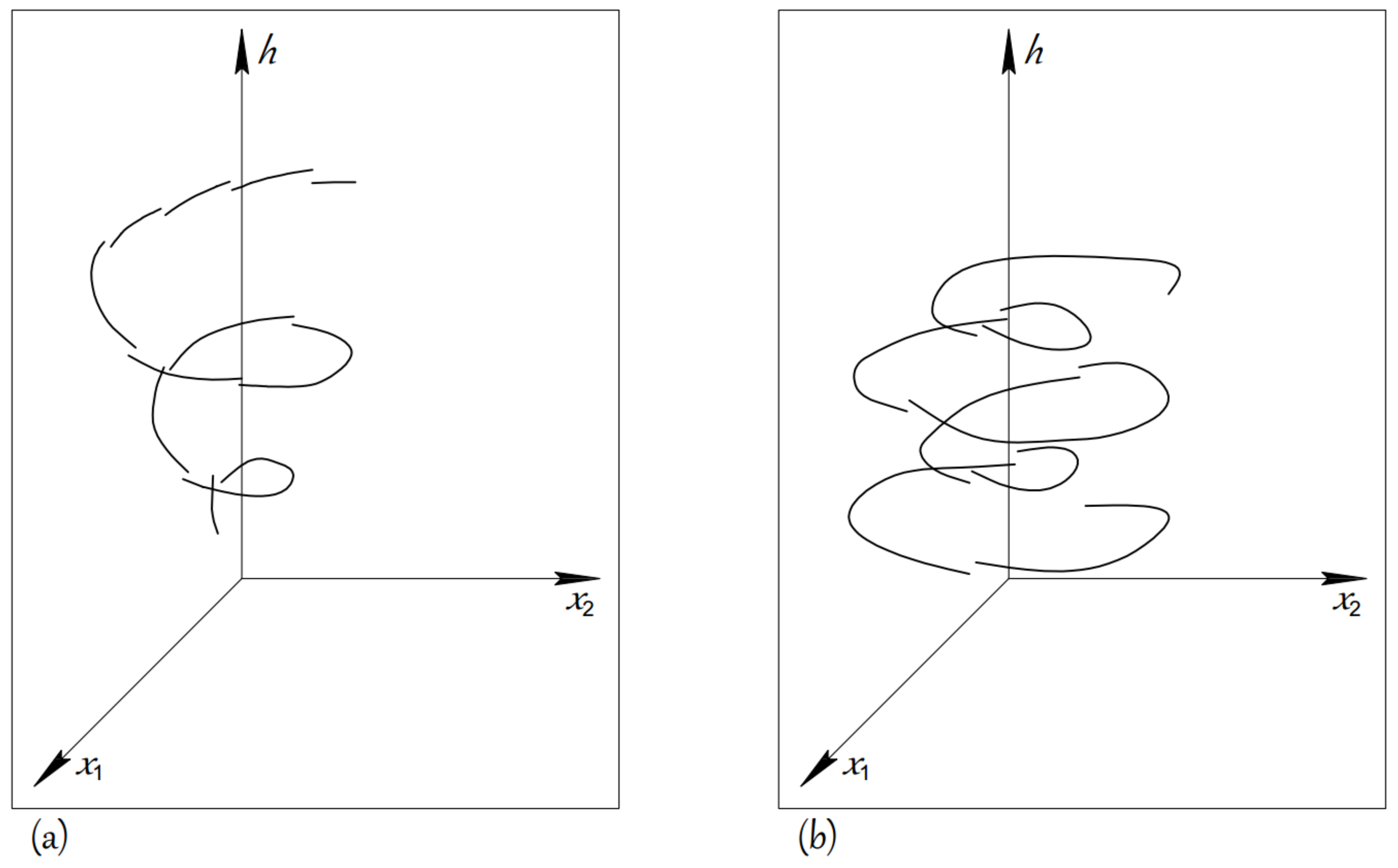
Example 1.

Consider the 2D impulsive control CNN with time-varying delays:

$$\left\{\begin{array}{ccc}{\dot{x}}_i\left(t\right)\hfill & =\hfill & {\displaystyle -c_i{x}_i\left(t\right)-\sum _{j=1}^2{a}_{ij}\left(t\right)f_j\left(x_j\left(t\right)\right)}\hfill \\ & & {\displaystyle -\sum _{j=1}^2{b}_{ij}\left(t\right)g_j\left(x_j(t-s_j\left(t\right))\right)-I_i,t\ne {\tau }_k\left(x\left(t\right)\right),}\hfill \\ & & i=1,2,k=1,2,\dots ,\hfill \end{array}\right.$$

(14)

with an impulsive control of the type:

$$\Delta x\left(t\right)=\left(\begin{array}{cc}-1+\frac{1}{k}\hfill & \hfill 0\\ 0\hfill & \hfill -1+\frac{1}{k}\end{array}\right)x\left(t\right),t={\tau }_k\left(x\left(t\right)\right),k=1,2,\dots ,$$

(15)

where:

$$\begin{array}{c}x\left(t\right)=\left(\begin{array}{c}{x}_1\left(t\right)\\ x_2\left(t\right)\end{array}\right),I_1=I_2=1,c_1=c_2=4,t_0=0,\\ {\displaystyle f_i\left(x\right)=g_i\left(x\right)=\frac{|x+1|-|x-1|}{2},0\le s_i\left(t\right)\le 1,}\\ a_{11}\left(t\right)=1.8-0.2sin\left(t\right),a_{12}\left(t\right)=0.3-0.4cos\left(t\right)-0.3sin\left(t\right),\\ a_{21}\left(t\right)=0.5+0.2cos\left(t\right)-0.3sin\left(t\right),a_{22}\left(t\right)=0.7-0.3sin\left(t\right),\\ b_{11}\left(t\right)=0.4sin\left(t\right),b_{12}\left(t\right)=0.2cos\left(t\right)+0.1sin\left(t\right),\\ b_{21}\left(t\right)=0.1cos\left(t\right)+0.2,b_{22}\left(t\right)=0.2sin\left(t\right),{\tau }_k\left(x\right)=\left|x\right|+k,k=1,2,\dots \end{array}$$

We have ${\tau }_k\in C[{\mathbb{R}}^2,(0,\infty )],k=1,2,\dots$, ${\tau }_k\left(x\right)\to \infty$ as $k\to \infty$ uniformly on $x\in R^2$, and also:

$$0<{\tau }_1\left(x\right)<{\tau }_2\left(x\right)<\dots ,x\in {\mathbb{R}}^2.$$

In addition, for the given choice of the functions ${\tau }_k$, conditions H2 and H3 are satisfied [9], and for $i=1,2$,

$$-1<P_{ik}=-1+\frac{1}{k}\le 0,k=1,2,\dots$$

Since:

$$\begin{array}{c}{a}_{11}^{+}=2,a_{12}^{+}=1,a_{21}^{+}=1,a_{22}^{+}=1,\\ b_{11}^{+}=0.4,b_{12}^{+}=0.3,b_{21}^{+}=0.3,b_{22}^{+}=0.2,\end{array}$$

then all conditions of Theorem 3 are satisfied for $M>1$ and $\mu \le 0.3$. We have that, for given $0<\lambda <A=11$ (for $M=2$ and $\mu =0.2$), the comparison problem (13) is $(\lambda ,A)$-globally practically exponentially stable. Hence, according to Theorem 3, the impulsive DCNN (14), (15) is $(\lambda ,A)$-globally practically exponentially stable with respect to the function $h=\sqrt{x_1^2+x_2^2}$. Especially, for $\lambda =9$, $A=11$, the simulation for the practically stable behavior is shown in Figure 1a.

Example 2.

If we again consider the impulsive CNN with time-varying delays (14), but with impulsive condition of the type:

$$\Delta x\left(t\right)=\Delta \left(\begin{array}{c}{x}_1\left(t\right)\\ x_2\left(t\right)\end{array}\right)=\left(\begin{array}{cc}-1+\frac{1}{k}\hfill & \hfill 0\\ 0\hfill & \hfill \frac{2}{k}\end{array}\right)x\left(t\right),t={\tau }_k\left(x\left(t\right)\right),k=1,2,\dots ,$$

(16)

we have that:

$$P_{2k}=\frac{2}{k}>0,k=1,2,\dots ,$$

and therefore, the impulsive perturbations do not guarantee the control of the practical stability behavior of (14). In this case, it is interesting to see that System (14) with impulses (16) is globally practically exponentially unstable with respect to the function $h=\sqrt{x_1^2+x_2^2}$, as is shown in Figure 1b.

Remark 5.

With our examples, we illustrated the established theoretical results. Furthermore, we again demonstrated that by means of appropriate impulsive perturbations, we can control the practical stability properties of CNNs. Since the practical stability with respect to h-manifolds is a generalization of many practical stability notions for CNNs and nonlinear systems, more generally, our results can be applied in the investigation of numerous applied problems.

5. Conclusions

In this paper, we extended the concept of the practical stability of impulsive control systems considering variable impulsive perturbations and h-manifolds. Since the notion of h-manifolds is much more general than that of trivial solutions, periodic solutions, equilibrium points, etc. our results generalized many existing practical stability criteria. Finally, we applied the obtained results to an impulsive neural network model with time-varying delays in order to illustrate the effectiveness of the developed approach. The generalized concept can be extended to study other types of impulsive control delayed systems.