Functions of Minimal Norm with the Given Set of Fourier Coefficients

Abstract

We prove the existence and uniqueness of the solution of the problem of the minimum norm function ${\parallel ·\parallel }_{\infty }$ with a given set of initial coefficients of the trigonometric Fourier series $c_j$, $j=0,1,\dots ,2n$. Then, we prove the existence and uniqueness of the solution of the nonnegative function problem with a given set of coefficients of the trigonometric Fourier series $c_j$, $j=1,\dots ,2n$ for the norm ${\parallel ·\parallel }_1$.

1. Introduction

The problem of the optimal continuation of a trigonometric polynomial in various spaces has been considered in many papers. This research began in the work of S. N. Bernstein [1]. One of the main questions here is to estimate the norm of a Fourier polynomial with some of its coefficients fixed. Here, we note the results of Schur [2] and Rahman and Schmeisser [3] on polynomials of minimal norm with some zero coefficients, leading to Chebyshev polynomials.

The problem of finding a Fourier polynomial with fixed coefficients with minimal norm ${\parallel f\parallel }_2$ is trivial. In [4], the problem of finding a Fourier polynomial of bounded degree with fixed coefficients with a minimum norm ${\parallel f\parallel }_{\infty }$ was solved. There are upper bounds for the norm ${\parallel ·\parallel }_{\infty }$ of trigonometric polynomials [5]. Estimates in the normalized spaces $L_p$, $p\in [1,+\infty ]$ were found in [6,7] by optimization methods in finite-dimensional spaces. In [5,8], it is shown that the optimal extension of an arbitrary trigonometric polynomial in the space $L^{\infty }[0,2\pi ]$ is unique and represents a step function of a constant modulus, but the proof was based on purely functional analytic methods and there was no indication of the way to construct the solutions. Thus, the first theorem of this paper presents another proof of this fact. The main purpose of our work is to introduce geometrical methods to solve these problems. This technique seems to be more illustrative than the purely analytic existence theorems in [8]. A rather large review of the results for polynomials and their derivatives with the fixed finite degree (trigonometric and power ones) of the minimum possible norm is given in [9]. For example, there exist numerous estimates of the polynomials norms through the norms of their derivatives in spaces $L^r(a,b)$ and $L^{\infty }(a,b)$, $a,b\in \mathbb{R}$, $r>1$.

In connection with the above results, one can note related problems of approximation by a polynomial bounded in the norm ${\parallel ·\parallel }_{\infty }$ of an analytic function in the unit circle of the complex plane [10,11]. When solving a number of problems, for example, the inverse problem of aerohydrodynamics, one has to use other norms [12,13,14]. Note that purely integral norms of the spaces $L^r(a,b)$ produce large pointwise values of the solution [13] and discontinuities result in singularities of the reconstructed contours [14].

In this paper, we generalize the results in [12,13], where the problems of the existence and uniqueness of the solution of the problem of the minimum norm function ${\parallel f\parallel }_{\infty }=\underset{t\in [0,2\pi ]}{\mathrm{ess}\sup }\left|f(t)\right|$, ${\parallel f\parallel }_1=\underset{0}{\overset{2\pi }{\int }}\left|f(t)\right|dt$ and ${\parallel f\parallel }_{\infty }+\lambda {\parallel f^{\prime }\parallel }_{\infty }$ (here, $\lambda$ is a fixed positive number) on the subclass of functions $C^1([0,2\pi ])$, with a given three first Fourier coefficients by a method other than the method in [4]. In the present paper, in a similar way, it is shown that the number of discontinuity points of the optimal function ${\varphi }^{*}$ for the norm ${\parallel ·\parallel }_{\infty }$ in [8] is not more than the double order of the original polynomial examples of finding the functions of the minimum norm and the solution of one such problem in the space of non-negative functions is constructed. This problem is naturally related to the classical moment problem (see, e.g., [15]). The last construction implies the uniqueness of the solution of the problem of the minimum norm function ${\parallel f\parallel }_1$ with the given three first Fourier coefficients, which clarifies the result in [4].

2. Results

2.1. The Function of the Minimum Norm ${\parallel ·\parallel }_{\infty }$ with a Given Set of Fourier Coefficients

Consider the following problem:

Find the function of the minimum norm ${\parallel ·\parallel }_{\infty }$ on the class of integrable functions $f:[0,2\pi ]\to \mathbb{R}$ with the given first $2n+1$ Fourier coefficients

$$c_{2j+1}=\frac{1}{2\pi }\underset{0}{\overset{2\pi }{\int }}f(t)\sin (jt)dt,c_{2j}=\frac{1}{2\pi }\underset{0}{\overset{2\pi }{\int }}f(t)\cos (jt)dt,j=0,1,\dots ,n.$$

Define the points ${\varphi }_1\le \dots \le {\varphi }_{2n}$ on the interval $[0,2\pi )$ and for an arbitrary constant $C\in \mathbb{R}$ consider the vector function

$$F(C,{\varphi }_1,{\varphi }_2,\dots ,{\varphi }_{2n})=2\left(\begin{array}{c}C({\displaystyle \sum _{k=1}^n}({\varphi }_{2k}-{\varphi }_{2k-1})-\pi )\\ C({\displaystyle \sum _{k=1}^n}(\sin ({\varphi }_{2k})-\sin ({\varphi }_{2k-1})))\\ ⋮\\ \frac{C}{n}({\displaystyle \sum _{j=1}^n}(\sin (n{\varphi }_{2k})-\sin (n{\varphi }_{2k-1})))\\ -C({\displaystyle \sum _{k=1}^n}(\cos ({\varphi }_{2k})-\cos ({\varphi }_{2k-1}))-1)\\ ⋮\\ -\frac{C}{n}({\displaystyle \sum _{k=1}^n}(\cos (n{\varphi }_{2k})-\cos (n{\varphi }_{2k-1}))-1).\end{array}\right)$$

Note that the coordinates of F are the Fourier coefficients of the locally constant function. Thus, the question is whether we can find the constant C and the angles ${\varphi }_1,\dots ,{\varphi }_{2n}$ so that $F^{\mathrm{tr}}=(c_0,c_1,\dots ,c_{2n})$.

We introduce on ${\mathbb{R}}^{+}\times {[0,2\pi )}^{2n}$ the equivalence relation $(C,{\varphi }_1,\dots ,{\varphi }_{j-1},\varphi ,\varphi ,{\varphi }_{j+2},\dots ,{\varphi }_{2n})\sim (C,{\varphi }_1,\dots ,{\varphi }_{j-1},\psi ,\psi ,{\varphi }_{j+2},\dots ,{\varphi }_{2n})$ with ${\varphi }_{j-1}<\varphi <{\varphi }_{j+2}$ and ${\varphi }_{j-1}<\psi <{\varphi }_{j+2}$. The function F takes the same value on elements of the same equivalence class. Consider the factor space $V={\mathbb{R}}^{+}\times {[0,2\pi )}^{2n}/\sim$.

Theorem 1.

The mapping $F:V\to {\mathbb{R}}^{2n+1}$ is a surjection.

Proof. 

Put $d_0=2{\displaystyle \sum _{j=1}^n}{\varphi }_{2j}-2{\displaystyle \sum _{j=1}^n}{\varphi }_{2j-1}-2\pi$, $d_k=2{\displaystyle \sum _{j=1}^n}\sin (k{\varphi }_{2j})-2{\displaystyle \sum _{j=1}^n}\sin (k{\varphi }_{2j-1})$, $d_{n+k}=-\frac{2}{n}{\displaystyle \sum _{j=1}^n}\cos (k{\varphi }_{2j})+\frac{2}{n}{\displaystyle \sum _{j=1}^n}\cos (k{\varphi }_{2j-1})-1$, $j=1,\dots ,n$. Then, the Jacobi matrix of the mapping F takes the form

$$J=\frac{\partial (c_0,c_1,\dots ,c_{2n})}{\partial (C,{\varphi }_1,\dots ,{\varphi }_{2n})}=$$

$$\left(\begin{array}{ccccc}{d}_0& 2C& -2C& \cdots & 2C\\ d_1& 2C\cos ({\varphi }_1)& -2C\cos ({\varphi }_2)& \cdots & -2C\cos ({\varphi }_{2n})\\ \dots \\ d_{2n}& -\frac{2C}{n}\sin (n{\varphi }_1)& \frac{2C}{n}\sin (n{\varphi }_2)& \cdots & \frac{2C}{n}\sin (n{\varphi }_{2n})\end{array}\right)$$

Note that C is a constant that scales an image of $F_1({\varphi }_1,\dots ,{\varphi }_{2n})=F(1,{\varphi }_1,\dots ,{\varphi }_{2n})$.

For $C=1$, the Jacobi matrix of the mapping $F_1$ is

$$J_1=\frac{\partial (c_0,c_1,\dots ,c_{2n})}{\partial ({\varphi }_1,\dots ,{\varphi }_{2n})}=$$

$$=-2\left(\begin{array}{cccc}1& -1& \cdots & 1\\ \cos ({\varphi }_1)& -\cos ({\varphi }_2)& \cdots & -\cos ({\varphi }_{2n})\\ \dots \\ \frac{1}{n}\cos (n{\varphi }_1)& -\frac{1}{n}\cos (n{\varphi }_2)& \cdots & -\frac{1}{n}\cos (n{\varphi }_{2n})\\ -\sin ({\varphi }_1)& \sin ({\varphi }_2)& \cdots & -\sin ({\varphi }_{2n})\\ \dots \\ -\frac{1}{n}\sin (n{\varphi }_1)& \frac{1}{n}\sin (n{\varphi }_2)& \cdots & \frac{1}{n}\sin (n{\varphi }_{2n})\end{array}\right).$$

Since an arbitrary string of n real elements sets the values of a trigonometric polynomial of order n at points ${\varphi }_1<\dots <{\varphi }_{2n}$, and the rows of this matrix form the basis values at the same points, the rank of this map is $2n$ when ${\varphi }_1<\dots <{\varphi }_{2n}$.

In the space ${\mathbb{R}}^{2n+1}$, we consider the hypersurface $F_1({[0,2\pi )}^{2n}/\sim )$. We show that in each direction $\overrightarrow{u}=(u_0,u_1,\dots ,u_{2n})$ in space ${\mathbb{R}}^{2n+1}$ there exist no more than two sets

$$\{{\varphi }_1,\dots ,{\varphi }_{2n}\},\{{\psi }_1={\varphi }_2,\dots ,{\psi }_{2n-1}={\varphi }_{2n},{\psi }_{2n}={\varphi }_1+2\pi \},$$

for which $D_{\overrightarrow{u}}F=(0,\dots ,0)$. Consider the trigonometric polynomial ${\displaystyle \sum _{j=0}^n}{u}_{2j}\cos j\varphi +{\displaystyle \sum _{j=1}^n}{u}_{2j-1}\sin j\varphi$, corresponding to the derivative in the direction $\overrightarrow{u}$, and find the roots of this polynomial. There exist at most $2n$ such roots.

Let there be exactly $2n$ of such roots. In this case, the set $\{{\varphi }_1,\dots ,{\varphi }_{2n}\}$ corresponds to a trigonometric polynomial of order n with roots ${\varphi }_1,\dots ,{\varphi }_{2n}$. The set $\{{\psi }_1,\dots ,{\psi }_{2n-1},{\psi }_{2n}\}$ represents the roots of a new polynomial obtained from the first polynomial by a change of sign.

If there exist fewer than $2n$ roots, then we get the roots $\{{\varphi }_1,\dots ,{\varphi }_{2n-2k}\}$ of the given polynomial and $\{{\psi }_1,\dots ,{\psi }_{2n-2k}\}$ are the roots of a polynomial obtained from the first one by change of sign.

This means that in any direction the derivative of the function $F_1$ has no more than two zeros. Thus, $F_1({[0,2\pi )}^{2n}/\sim )$ is a convex hypersurface.

Note that the hypersurface $F_1({[0,2\pi )}^{2n}/\sim )$ is symmetric about the origin by construction, because $F_1({\varphi }_1,\dots ,{\varphi }_{2n})=-F_1({\varphi }_2,\dots ,{\varphi }_{2n},{\varphi }_1+2\pi )$ and compact, since each coordinate is bounded in ${\mathbb{R}}^{2n+1}$.

Thus, we have the following:

• The Jacobian $F_1$ is not zero on the hypersurface $F_1({[0,2\pi )}^{2n}/\sim )$ with ${\varphi }_1<{\varphi }_2<\dots <{\varphi }_{2n}$ and $C\ne 0$.
• The Jacobian $F_1$ is zero on the hypersurface $F_1({[0,2\pi )}^{2n}/\sim )$ on a subset of dimension $2n-1=\dim (V)-2$, and the degeneration of the map occurs with ${\varphi }_j={\varphi }_{j+1}$.

Since the mapping $F_1$ is continuous, its image is closed on the hypersurface $F_1({[0,2\pi )}^{2n}/\sim )$. Item 1 implies that this hypersurface has dimension $2n$. Item 2 yields that the dimension of the boundary of this image is $2n-2$. Consequently, the image of $F_1$ is a manifold of dimension $2n$ without an edge.

Consequently, the image of $F_1$ is a convex surface that is homotopy equivalent to the sphere ${\mathbb{S}}^{2n}\subset {\mathbb{R}}^{2n+1}$.

Therefore, for any point $w\in {\mathbb{R}}^{2n+1}$ exist a number $C\in {\mathbb{R}}^{+}$ and a set ${\varphi }_1\le \dots \le {\varphi }_{2n}$ such that $w=F(C,{\varphi }_1,\dots ,{\varphi }_{2n})=CF(1,{\varphi }_1,\dots ,{\varphi }_{2n})$. □

Corollary 1.

For each set of Fourier coefficients, there exists a piecewise constant, constant modulo function with a given set of first coefficients.

Proof. 

Since the components of the vector function $F(C,{\varphi }_1,\dots ,{\varphi }_{2n})$ introduced in Theorem 1 are the Fourier coefficients of the piecewise constant function

$$f(t)=\left\{\begin{array}{cc}C,& t\in ({\varphi }_{2j},{\varphi }_{2j+1}],\\ -C,& t\in ({\varphi }_{2j-1},{\varphi }_{2j}]\end{array}\right.j=1,\dots ,n,{\varphi }_{2n+1}={\varphi }_1,$$

(1)

in accordance with Theorem 1, we obtain the proof of this statement. □

Theorem 2.

For any set $(c_0,\dots ,c_{2n})\in {\mathbb{R}}^{2n+1}$ there exists a unique function (Equation (1)) that minimizes the norm ${\parallel ·\parallel }_{\infty }$.

Proof. 

In accordance with Corollary 1, for a given set of Fourier coefficients $(c_0,\dots ,c_{2n})$, we choose a piecewise constant, where $C_1$ is the minimal possible number from the preimages $F^{-1}(c_0,\dots ,c_{2n})$.

Assume that there exists a function $f_2$ less than or equal to the norm of ${\parallel ·\parallel }_{\infty }$, with the same set of coefficients.

Consider the difference of two functions $f_1$, $f_2$ with a given set of first Fourier coefficients. Since the first $2n+1$ Fourier coefficients are 0, this function has the form $f_2(t)-f_1(t)=\mathrm{Re}\left[e^{i(n+1)t}h(e^{it})\right]$, where $h(z)$ is a function that is holomorphic in the unit circle. Consequently, in accordance with the principle of the argument, the difference $f_2(t)-f_1(t)$ changes sign not fewer than $2n+2$ times. Since $\parallel f_2{(t)\parallel }_{\infty }\le {\parallel f_1(t)\parallel }_{\infty }$, we have $f_2(t)-f_1(t)\le 0$, $t\in [{\varphi }_{2j-1},{\varphi }_{2j})$, $f_2(t)-f_1(t)\ge 0$, $t\in [{\varphi }_{2j},{\varphi }_{2j+1})$, $j=1,\dots ,n$, ${\varphi }_{2j+1}={\varphi }_1$. That is, the difference $f_2(t)-f_1(t)$ changes sign no more than $2n$ times. The contradiction confirms that the function $f_1$ has a minimal norm.

Uniqueness of this function on the class of functions of the form of Equation (1) follows from the same considerations. Let there be another piecewise-constant function with a constant module $f_2$ with the same first Fourier coefficients in accordance with Corollary 1. Then, $C_2=C_1$ and from the already proved, it follows that the set $\{{\varphi }_1,\dots ,{\varphi }_{2n}\}$ for the function $f_2$ coincides with the corresponding set for $f_1$. □

From Theorems 1 and 2, it follows that F is a global homeomorphism and C is the minimum norm of the function, the first $2n+1$ of the Fourier coefficients of which are $c_0,\dots ,c_{2n}$.

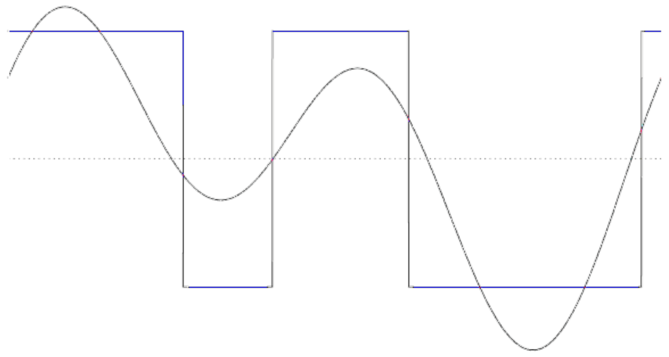
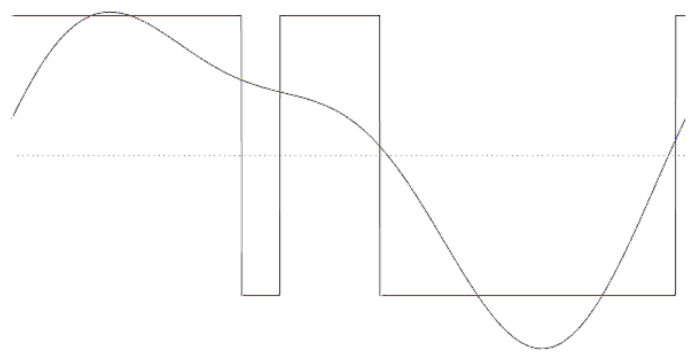
Let us give examples illustrating the results of Theorem 2 for the case $n=2$. We construct piecewise constant functions that provide the minimum norm for given trigonometric polynomials. The examples are constructed by selecting the values ${\varphi }_k$, $k=1,\dots ,4$ so that the ratio of the Fourier coefficients of a constant modulo function is the same as that of the original polynomial. Figure 1 and Figure 2 show the graphs of both approximate and corresponding constant modulo functions with $C=1.538$ and $C=3.713$, respectively.

Consider the function $g\in C([0,2\pi ))$ and the sequence $c_{2j-1}=\frac{1}{2\pi }\underset{0}{\overset{2\pi }{\int }}g(t)\sin (jt)dt$, $c_{2j}=\frac{1}{2\pi }\underset{0}{\overset{2\pi }{\int }}g(t)\cos (jt)dt$, $j\in \mathbb{N}$. Then, we have functions of the type (1) $f_n(t)$, $t\in [0,2\pi ]$ of minimal norm $\parallel f_n{\parallel }_{\infty }$ for polynomials $g_n(t)={\displaystyle \sum _{j=0}^n}[c_{2j}\cos (jt)+c_{2j+1}\sin (jt)]$.

This leads us to the following statements.

Corollary 2.

$\parallel f_n{\parallel }_{\infty }\to {\parallel g\parallel }_{\infty }$, ($n\to \infty$).

Proof. 

Assume the contrary. Since, for each n, $f_n(t)$ is a function of the minimum possible norm for a given set of Fourier coefficients of the function g, the sequence of norms $\{\parallel f_n{\parallel \}}_{n=1}^{\infty }$ is marorized by the sequence of norms $\{\parallel g_n{{\parallel }_{\infty }\}}_{n=1}^{\infty }$. In addition, since $f_{n+1}(t)$ is constructed according to a larger number of given Fourier coefficients than $f_n(t)$, $\parallel f_n{\parallel }_{\infty }\le {\parallel f_{n+1}\parallel }_{\infty }$. Consequently, the sequence $\{\parallel f_n{\parallel \}}_{n=1}^{\infty }$ is monotone and bounded above, that is, converges. Let $\parallel f_n{\parallel }_{\infty }\to D$, ($n\to \infty$). By assumption, ${D<\parallel g\parallel }_{\infty }$. Consider

$$h(t)=\left\{\begin{array}{cc}g(t)-D,& g(t)>D,\\ g(t)+D,& g(t)<-D,\\ 0,& |g(t)|<D.\end{array}\right.$$

The function $h(t)$ realizes the minimal distance from the function $g(t)$ to a convex set of functions modulo less than D. Consider the finite sum of the Fourier series $h_0(t)$ for $h(t)$, $\parallel h_0{\parallel }_2={\epsilon }_0$. Then, there is $K\in \mathbb{N}$ such that for any $n>K$, $\parallel g-f_n{\parallel }_2\ge {\parallel h_0\parallel }_2={\epsilon }_0$. Consequently, any finite-dimensional subset of a convex set of functions modulo less than D is at a distance not less than ${\epsilon }_0$ from $h_0$. Therefore, the Fourier coefficients $f_n(t)$ are separated from the coefficients $g(t)$ starting from a certain number. This contradicts the assumption that the first $2n+1$ Fourier coefficients for $f_n(t)$ and $g_n(t)$ coincide. □

We now easily infer the following.

Corollary 3.

$f_n(t)\to g(t)$ by the norm ${\parallel ·\parallel }_{\infty }$, ($n\to \infty$) ⇔$g=\{\pm C\}$.

Examples from [4] show the convergence of polynomials to step functions, which are solutions to the problem as the degree of polynomials tends to ∞.

2.2. The Function of the Minimum Norm ${\parallel f\parallel }_{\infty }+\lambda {\parallel f^{\prime }\parallel }_{\infty }$ with a Given Set of Fourier Coefficients

Consider the sequence of functions of the form

$$f(t)=\left\{\begin{array}{cc}C(1-e^{-\frac{t-{\varphi }_{2k}}{\lambda }}),& t\in [{\varphi }_{2k},\frac{{\varphi }_{2k}+{\varphi }_{2k+1}}{2}],\\ C(1-e^{\frac{t-{\varphi }_{2k+1}}{\lambda }}),& t\in [\frac{{\varphi }_{2k}+{\varphi }_{2k+1}}{2},{\varphi }_{2k+1}],\\ -C(1-e^{-\frac{t-{\varphi }_{2k-1}}{\lambda }}),& t\in [{\varphi }_{2k-1},\frac{{\varphi }_{2k}+{\varphi }_{2k-1}}{2}],\\ -C(1-e^{\frac{t-{\varphi }_{2k}}{\lambda }}),& t\in [\frac{{\varphi }_{2k}+{\varphi }_{2k-1}}{2},{\varphi }_{2k}]\end{array}\right.j=1,\dots ,n,{\varphi }_{2n+1}={\varphi }_1,$$

where, for any k${\varphi }_{2k}\le {\varphi }_{2k+2}$, ${\varphi }_{2k-1}\le {\varphi }_{2k+1}$.

Then, again, similar to the previous section, we have a diffeomorphism of the set $M=\left\{(C,{\varphi }_1,\dots ,{\varphi }_{2n})\right\}/\simeq$ onto ${\mathbb{R}}^{2n+1}$. Once again, existence follows from the fact that the dimension of the boundary of M is $2n-1$. The mapping Jacobian is equal to the mapping Jacobian from the previous item multiplied by ${(-1)}^n{C}^n{\displaystyle \prod _{k=1}^{2n}}(1-e^{-\frac{{\varphi }_k}{\lambda }})$. Indeed, the Jacobi matrix of the mapping equals

$$J_2=\frac{\partial (c_0,c_1,\dots ,c_{2n})}{\partial ({\varphi }_1,\dots ,{\varphi }_{2n})}=$$

$$=-2\pi \left(\begin{array}{cccc}(1-e^{-\frac{{\varphi }_1}{\lambda }})& -(1-e^{-\frac{{\varphi }_2}{\lambda }})& \cdots & -(1-e^{-\frac{{\varphi }_{2n}}{\lambda }})\\ (1-e^{-\frac{{\varphi }_1}{\lambda }})\sin ({\varphi }_1)& -(1-e^{-\frac{{\varphi }_2}{\lambda }})\sin ({\varphi }_2)& \cdots & -(1-e^{-\frac{{\varphi }_{2n}}{\lambda }})\sin ({\varphi }_{2n})\\ \dots \\ \frac{1-e^{-\frac{{\varphi }_1}{\lambda }}}{n}\sin (n{\varphi }_1)& -\frac{1-e^{-\frac{{\varphi }_2}{\lambda }}}{n}\sin (n{\varphi }_2)& \cdots & -\frac{1-e^{-\frac{{\varphi }_{2n}}{\lambda }}}{n}\sin (n{\varphi }_{2n})\\ -(1-e^{-\frac{{\varphi }_1}{\lambda }})\cos ({\varphi }_1)& (1-e^{-\frac{{\varphi }_2}{\lambda }})\cos ({\varphi }_2)& \cdots & -(1-e^{-\frac{{\varphi }_{2n}}{\lambda }})\cos ({\varphi }_{2n})\\ \dots \\ -\frac{1-e^{-\frac{{\varphi }_1}{\lambda }}}{n}\cos (n{\varphi }_1)& \frac{1-e^{-\frac{{\varphi }_2}{\lambda }}}{n}\cos (n{\varphi }_2)& \cdots & \frac{1-e^{-\frac{{\varphi }_{2n}}{\lambda }})}{n}\cos (n{\varphi }_{2n})\end{array}\right).$$

2.3. The Function of the Minimum Norm ${\parallel ·\parallel }_1$ with a Given Set of Fourier Coefficients

Consider the following problem.

On the class of non-negative integrable functions $f:[0,2\pi ]\to {\mathbb{R}}^{+}$ with the given $2n$ Fourier coefficients

$$c_{2j+1}=\frac{1}{2\pi }\underset{0}{\overset{2\pi }{\int }}f(t)\sin (jt)dt,c_{2j}=\frac{1}{2\pi }\underset{0}{\overset{2\pi }{\int }}f(t)\cos (jt)dt,j=0,\dots ,n,$$

find the function of the minimum norm ${\parallel ·\parallel }_1$.

Consider the function

$$g(t)=\sum _{k=1}^n{a}_k{\delta }_{{\varphi }_k}(t),a_k\ge 0,{\varphi }_k\in [0,2\pi ).$$

(2)

Here, ${\delta }_{{\varphi }_k}(t)$ is the Kronecker $\delta$-function.

Theorem 3.

For any set $(c_1,\dots ,c_{2n})\in {\mathbb{R}}^{2n}$, there is a unique function $g(t)$ of the form in Equation (2), which is a solution of the formulated problem.

Proof. 

The proof of the statement is based on the same considerations as in the case of the problem for the norm ${\parallel ·\parallel }_{\infty }$.

Existence. As in Theorem 1, we show the degeneration of the mapping image boundary.

$$G_1(a_1,\dots ,a_n,{\varphi }_1,{\varphi }_2,\dots ,{\varphi }_n)=\left(\begin{array}{c}{\displaystyle \sum _{j=1}^n}{a}_j{e}^{i{\varphi }_j}\\ {\displaystyle \sum _{j=1}^n}{a}_j{e}^{i2{\varphi }_j}\\ ⋮\\ {\displaystyle \sum _{j=1}^n}{a}_j{e}^{in{\varphi }_j}\end{array}\right).$$

For ${\varphi }_1<\dots <{\varphi }_n$, the map Jacobian is non-degenerate, since it is a multiple of the determinant of the Vandermond matrix $V(e^{i{\varphi }_1},\dots ,e^{i{\varphi }_n})$. The Jacobi matrix of the mapping $G_1$ is a block matrix of the form

$$J=\frac{\partial c_1,\dots ,c_{2n}}{\partial {\varphi }_1,\dots ,{\varphi }_n,a_1,\dots ,a_n}=\left(\begin{array}{cc}A& B\\ -B^{\prime }& A^{\prime }\end{array}\right).$$

Here,

$$A=\left(\begin{array}{ccc}\sin {\varphi }_1& \dots & \sin {\varphi }_n\\ \dots \\ \sin n{\varphi }_1& \dots & \sin n{\varphi }_n\end{array}\right),A^{\prime }=\left(\begin{array}{ccc}{a}_1\sin {\varphi }_1& \dots & a_n\sin {\varphi }_n\\ \dots \\ n{a}_1\sin n{\varphi }_1& \dots & n{a}_n\sin n{\varphi }_n\end{array}\right).$$

$$B=\left(\begin{array}{ccc}\cos {\varphi }_1& \dots & \cos {\varphi }_n\\ \dots \\ \cos n{\varphi }_1& \dots & \cos n{\varphi }_n\end{array}\right),B^{\prime }=\left(\begin{array}{ccc}{a}_1\cos {\varphi }_1& \dots & a_n\cos {\varphi }_n\\ \dots \\ n{a}_1\cos n{\varphi }_1& \dots & n{a}_n\cos n{\varphi }_n\end{array}\right).$$

This matrix is non-degenerate if and only if the Jacobi matrix $n!{\displaystyle \prod _{j=1}^n}{a}_j(A+iB):{\mathbb{C}}^n\to {\mathbb{C}}^n$ of the mapping $J:{\mathbb{R}}^{2n}\to {\mathbb{R}}^{2n}$ complexified with the affinor $I=\left(\begin{array}{cc}0& I_n\\ -I_n& 0\end{array}\right)$ is degenerate. This is true for $a_j=0$, $j\in \{1,\dots ,n\}$ or for ${\varphi }_j={\varphi }_k$, $j\ne k\in \{1,\dots ,n\}$. The image of $G_1({({\mathbb{R}}^{+})}^n\times {[0,2\pi )}^n)$ is a subset of dimension $2n$ with boundary of dimension $2n-2$ of space ${\mathbb{R}}^{2n}$. Then, $G_1({({\mathbb{R}}^{+})}^n\times {[0,2\pi )}^n)={\mathbb{R}}^{2n}$.

Further, similar to the proof of Theorem 2, we prove the uniqueness of the pre-image for the mapping $G_1$.

Assume that there exist two different solutions $g_1(t)$ and $g_2(t)$. Consider $g_3(t,K)=g_1(t)-g_2(t)+K$, $K\in \mathbb{R}$. On the one hand, for some $K_0$, the function $g_3(t,K_0)$ has at least $2n+2$ sign changes. On the other hand, $g_3(t,K)$ has at most $2n$ sign changes for any K. We arrive at a contradiction. □

We now consider the problem of finding the function of the minimum norm ${\parallel ·\parallel }_1$ satisfying the conditions

(1)

$f(t)\in L^2([0,2\pi ])$; and

(2)

$\underset{0}{\overset{2\pi }{\int }}f(t)e^{ijt}dt=c_j$, $c_j\in \mathbb{C}$, $j=0,\dots ,n$, $c_0\in \mathbb{R}$.

Consider the function

$$H(t)=\sum _{k=1}^{2n}{a}_k{\delta }_{{\varphi }_k}(t),a_k\in \mathbb{R},{\varphi }_k\in [0,2\pi ).$$

(3)

Corollary 4.

For any set $(c_0,c_1\dots ,c_n)\in \mathbb{R}\times {\mathbb{C}}^n$, there exists a function of the form in Equation (3) satisfying Conditions (1) and (2).

We construct the function $g_1(t)$ from Theorem 3 by the set of coefficients $(c_1\dots ,c_n)$ and the function $g_2(t)$ by the set of coefficients $(-c_1\dots ,-c_n)$ and select $\lambda \in \mathbb{R}$ so that $\underset{0}{\overset{2\pi }{\int }}{g}_3(t)dt=\underset{0}{\overset{2\pi }{\int }}\lambda g_1(t)+(1-\lambda )(-g_2(t))dt=c_0$.

Note that for $n=1$ the solution to the last problem is $H(t)$ [12].

Example. Consider the polynomial $1+2\cos t$. Then, the first term in Corollary 4 is of the form $4\pi {\delta }_0(t)$, and the second equals $4\pi {\delta }_{\pi }(t)$. We have $k=5/8$ and $H(t)=\frac{5\pi }{2}{\delta }_0(t)-\frac{3\pi }{2}{\delta }_{\pi }(t)$.

2.4. Figures, Tables and Schemes

The Figure 1 and Figure 2 are as follows:

3. Discussion

The results presented here may be applied for constructing multi-connected wing profiles in aerohydrodynamics as well as in the study of cavitation diagrams. In addition, we introduce a new technique for solution of similar problems.

4. Materials and Methods

All the constructions of examples were performed in Maxima and are available on the first request.

5. Conclusions

Here, we solved some problems of conditional approximation introducing new proof methods. Note that the problem of uniqueness of nonnegative solution for the space $L^1(0,2\pi )$ in the general case is yet unsolved.

These results can be applied to different optimization problems of mathematical physics. For example, in aerohydrodynamics, a wing may be considered as the set of parallel profiles [16], thus, to optimize the wing contour, we need to simultaneously optimize the contours bounding these profiles. Recall that the problem for the norm ${\parallel f\parallel }_{\infty }+\lambda {\parallel f^{\prime }\parallel }_{\infty }$ appeared due to the following reasons: (1) the integral norms generate solutions too different from the initial velocity distribution; and (2) discontinuous solutions involve reconstruction of contours with singularities.

These methods are applicable to not necessarily one-dimensional problems. Again, to include in our considerations the air shift along the wing blade, we do not need to optimize the wing sections in two mutually orthogonal directions. It also seems possible to prove certain inequalities of complex analysis with the help of these methods.

References

- Bernstein, S.; de la Vallée Poussin, C. L’approximation; Chelsea Publishing Comp: Bronx, NY, USA, 1970. [Google Scholar]
- Schur, I. Uber das Maximum des absoluten Betrages ernes Polynoms in einem gegebenen Interval. Math. Z. 1919, 4, 271–287. [Google Scholar] [CrossRef]
- Rahman, Q.I.; Schmeisser, G. Les inégalités de Markoff et de Bernstein; Presses Univ. Montreal: Montreal, QC, Canada, 1983. [Google Scholar]
- Dette, H.; Melas, V.B. A note on some extremal problems for trigonometric polynomials, No 2005, 20. In Technical Reports from Technische Universitaet Dortmund, Sonderforschungsbereich 475: Komplexitaetsreduktion in multivariaten Datenstrukturen; EconStor: Kiel, Germany, 2005; pp. 1–17. [Google Scholar]
- Taikov, L.V. On the best approximation of Dirichlet kernels. Math. Notes 1993, 53, 640–643. [Google Scholar] [CrossRef]
- Hesse, K.; Sloan, I.H. Hyperinterpolation on the Sphere. In Frontiers in Interpolation and Approximation; Govil, N.K., Mhaskar, H.N., Mohapatra, R.N., Nashed, Z., Szabados, J., Eds.; Taylor and Frances: Didcot, UK, 2007; pp. 213–248. [Google Scholar]
- Ash, J.M.; Ganzburg, M. An extremal problem for trigonometric polynomials. Proc. AMS 1999, 127, 211–216. [Google Scholar] [CrossRef]
- Taikov, L.V. On a group of extremal problems for trigonometric polynomials. Usp. Mat. Nauk 1965, 20, 205–211. [Google Scholar]
- Milovanovic, G.V.; Rassias, T.M.; Mitrinovic, D.S. Topics in Polynomials: Extremal Problems, Inequalities, Zeros; World Scientific: Singapore, 1999. [Google Scholar]
- Babenko, K.I. Ueber die besten Approximationen einer Klasse analytischer Funktionen. Izv. Akad. Nauk SSSR Ser. Mat. 1958, 22, 631–640. (In Russian) [Google Scholar]
- Goluzin, G.M. Geometric Theory of Functions of a Complex Variable; Translations of Mathematical Monographs; American Mathematical Society: Providence, RI, USA, 1969; Volume 26. [Google Scholar]
- Ivanshin, P.N. Quasisolutions of one inverse boundary-value problem of aerohydromechanics. Russ. Math. 2013, 57, 9–19. [Google Scholar] [CrossRef]
- Ivanshin, P.N. Conditional Optimization and One Inverse Boundary Value Problem. Math. Probl. Eng. 2015, 2015, 949703. [Google Scholar] [CrossRef]
- Avkhadiev, F.G.; Elizarov, A.M. Exact bounds of solution to a variation inverse boundary value problem in a countable-connected domain. Russ. Math. 1996, 40, 1–11. [Google Scholar]
- Berg, C.; Szwarc, R. A determinant characterization of moment sequences with finitely many mass points. Linear Multilinear Algebra 2015, 63, 1568–1576. [Google Scholar] [CrossRef]
- Sadrehaghighi, I. Aerodynamic Design & Optimization; ResearchGate: Berlin, Germany, 2019. [Google Scholar] [CrossRef]
Figure 1.
The function and the function of the minimum norm with the same set of first five Fourier coefficients.
Figure 2.
© 2019 by the author. Licensee MDPI, Basel, Switzerland. This article is an open access article distributed under the terms and conditions of the Creative Commons Attribution (CC BY) license (http://creativecommons.org/licenses/by/4.0/).
Share and Cite
MDPI and ACS Style
Ivanshin, P. Functions of Minimal Norm with the Given Set of Fourier Coefficients. Mathematics 2019, 7, 651. https://doi.org/10.3390/math7070651
AMA Style
Ivanshin P. Functions of Minimal Norm with the Given Set of Fourier Coefficients. Mathematics. 2019; 7(7):651. https://doi.org/10.3390/math7070651
Chicago/Turabian StyleIvanshin, Pyotr. 2019. "Functions of Minimal Norm with the Given Set of Fourier Coefficients" Mathematics 7, no. 7: 651. https://doi.org/10.3390/math7070651
Note that from the first issue of 2016, this journal uses article numbers instead of page numbers. See further details here.