Linear Convergence of an Iterative Algorithm for Solving the Multiple-Sets Split Feasibility Problem

Abstract

In this paper, we propose the simultaneous sub-gradient projection algorithm with the dynamic step size (SSPA for short) for solving the multiple-sets split feasibility problem (MSSFP for short) and investigate its linear convergence. We involve a notion of bounded linear regularity for the MSSFP and construct several sufficient conditions to prove the linear convergence for the SSPA. In particular, the SSPA is an easily calculated algorithm that uses orthogonal projection onto half-spaces. Furthermore, some numerical results are provided to verify the effectiveness of our proposed algorithm.

1. Introduction

Let $H_1$ and $H_2$ be two Hilbert spaces, $C\subseteq H_1$ and $Q\subseteq H_2$ be two closed, convex and nonempty sets. Let operator $A:H_1\to H_2$ be bounded and linear. The split feasibility problem (SFP for short) was proposed by Censor and Elfving [1] to solve the phase retrieval problems, and is formulated as:

$$\mathrm{finding}x\in C\mathrm{and}y\in Q\mathrm{such}\mathrm{that}Ax=y.$$

(1)

Let $\overline{S}=C\times Q\subseteq H=H_1\times H_2$, $G=[A,-I]:H\to H_2$, $G^{*}$ be the adjoint operator of G, then SFP (1) can be reformulated as:

$$\mathrm{finding}w=(x,y)\in \overline{S}\mathrm{such}\mathrm{that}Gw=0.$$

(2)

This class of problem has received plenty of attention due to its wide applications, such as intensity-modulated radiation therapy [2], signal processing [3], image reconstruction [4], etc.

Many algorithms have been developed to solve the SFP. One of the most popular and practical algorithms is the CQ algorithm, which was proposed by Byrne [5]:

$$x_{n+1}=P_C(x_n-\gamma A^{*}(I-P_Q)A{x}_n),$$

where $A^{*}$ is the adjoint operator of A, $\gamma >0$ is the step size, while $P_C$ and $P_Q$ denote the orthogonal projection onto C and Q, respectively.

As a quite important generalization of the CQ algorithm, López et al. [6] introduced the following dynamic step size CQ algorithm and obtained a weak convergence result:

$$x_{n+1}=P_C(x_n-{\gamma }_n{A}^{*}(I-P_Q)A{x}_n),$$

where

$${\gamma }_n=\left\{\begin{array}{c}0,x_n\in C\cap A^{-1}Q;\hfill \\ \frac{{\rho }_n{\parallel (I-P_Q)Ax\parallel }^2}{\parallel A^{*}(I-P_Q){Ax\parallel }^2}and{\rho }_n\subseteq (0,2),otherwise.\hfill \end{array}\right.$$

The highlight of the dynamic step size CQ algorithm is that it does not require any prior knowledge about the norm of the operator A.

Under some additional assumptions, the strong convergence property of the CQ algorithm was developed in [7] as special cases of some generalized CQ-type algorithms. More papers about this topic are given [8,9] and the references therein. However, there are few results involving the rate of convergence.

In this paper, we investigate the multiple-sets split feasibility problem (MSSFP), which is to find a point such that:

$$x\in C=\bigcap _{i=1}^t{C}_i,Ax\in Q=\bigcap _{j=1}^r{Q}_j,$$

(3)

where r and t are positive integers; ${\left\{C_i\right\}}_{i=1}^t$ and ${\left\{Q_j\right\}}_{j=1}^r$ are closed, convex and nonempty subsets of Hilbert spaces $H_1$ and $H_2$, respectively; $A:H_1\to H_2$ is a bounded linear operator. Without loss of generality, suppose that $t>r$, and choose $Q_{r+1}=Q_{r+2}=\cdots =Q_t=H_2$. Let $S_i=C_i\times Q_i\subseteq \tilde{H}=H_1\times H_2$, $i=1,2,\cdots ,t$, $\widehat{S}=\bigcap _{i=1}^t{S}_i$, $G=[A,-I]:\tilde{H}\to H_2$, $G^{*}$ be the adjoint operator of G. Then MSSFP (3) can be reformulated as:

$$\mathrm{finding}w=(x,y)\in \widehat{S}\mathrm{such}\mathrm{that}Gw=0.$$

(4)

Censor et al. [10] proposed the following iterative formula by using the projection gradient method for solving the MSSFP:

$$x_{n+1}=P_{\mathsf{\Omega }}[x_n-s(\sum _{i=1}^t{\alpha }_i(x_n-P_{C_i}{x}_n)+\sum _{j=1}^r{\beta }_j{A}^{*}(A{x}_n-P_{Q_j}A{x}_n)],$$

where $\mathsf{\Omega }\subset R^N$ is an auxiliary simple set, $s\in (0,\frac{2}{L}),L={\displaystyle \sum _{i=1}^t}{\alpha }_i+\varrho \left(A^{*}A\right){\displaystyle \sum _{j=1}^r}{\beta }_j$, $\varrho \left(A^{*}A\right)$ is the spectral radius of $A^{*}A$, ${\displaystyle \sum _{i=1}^t}{\alpha }_i+{\displaystyle \sum _{j=1}^r}{\beta }_j=1$ with ${\alpha }_i>0$, ${\beta }_j>0$. However, this algorithm is usually difficult to calculate. Then, Censor et al. [11] developed the following simultaneous sub-gradient projection algorithm, which is an easily calculated algorithm that uses orthogonal projection onto half-spaces, to solve the MSSFP:

$$x_{n+1}=x_n-\frac{s}{L}[\sum _{i=1}^t{\alpha }_i(x_n-P_{C_{i,n}}{x}_n)+\sum _{j=1}^r{\beta }_j{A}^{*}(A{x}_n-P_{Q_{j,n}}A{x}_n)].$$

Here, $s\in (0,2),L={\displaystyle \sum _{i=1}^t}{\alpha }_i+\varrho \left(A^{*}A\right){\displaystyle \sum _{j=1}^r}{\beta }_j$, $\varrho \left(A^{*}A\right)$ is the spectral radius of $A^{*}A$, ${\displaystyle \sum _{i=1}^t}{\alpha }_i+{\displaystyle \sum _{j=1}^r}{\beta }_j=1$ with ${\alpha }_i>0$, ${\beta }_j>0$ and:

$$C_{i,n}:=\{x\in H_1:c_i\left(x_n\right)+\langle {\xi }_{i,n},x-x_n\rangle \le 0\},$$

where ${\xi }_{i,n}\in \partial c_i\left(x_n\right)$, $i=1,2,\cdots ,t$, and:

$$Q_{j,n}:=\{y\in H_2:q_j\left(y_n\right)+\langle {\eta }_{j,n},y-y_n\rangle \le 0\},$$

where ${\eta }_{j,n}\in \partial q_j\left(y_n\right)$, $j=1,2,\cdots ,r$. However, the above projection method with a fixed step size may be very slow. Then, motivated by the extrapolated method for solving the convex feasibility problems in [12], Dang et al. [13] proposed a simultaneous sub-gradient projection algorithm to solve the MSSFP by utilizing two extrapolated factors in one iterative step. We remark here that the above algorithms only converge weakly to a solution of the MSSFP. Moreover, the rate of convergence has not been explicitly estimated. Based on the above disadvantages, we propose a simultaneous sub-gradient projection algorithm with the dynamic step size (SSPA for short) for solving the MSSFP by utilizing projections onto half-spaces to replace the original convex sets, and we investigate the linear convergence of the SSPA. Furthermore, we conclude the linear convergence rate of the SSPA.

The rest of this paper is organized as follows. Section 2 introduces the concept of bounded linear regularity for the MSSFP and presents some relevant definitions and lemmas which will be very useful for our convergence analysis. Section 3 gives the SSPA, the proof of its linear convergence and its linear convergence rate. Section 4 presents some numerical results to clarify the validity of our proposed algorithm.

2. Preliminaries

For convenience, we always suppose that H is a real Hilbert space with the inner product $\langle ·,·\rangle$ and the norm $\parallel ·\parallel$. I denotes the identity operator on H. For a set $C\subseteq H$, $\mathrm{int}C$ denotes the interior of C. We denote by $\mathbf{B}$ and $\overline{\mathbf{B}}$ as the unit open metric ball and unit closed metric ball with center at the origin, respectively, that is:

$$\mathbf{B}:=\{x\in H:\parallel x\parallel <1\}\mathrm{and}\overline{\mathbf{B}}:=\{x\in H:\parallel x\parallel \le 1\}.$$

For a point $x\in H$ and a set $C\subseteq H$, the orthogonal projection of x onto C and the distance of x from C, denoted by $P_C\left(x\right)$ and $d_C\left(x\right)$, are respectively defined by:

$$P_C\left(x\right):=argmin\{\parallel x-y\parallel :y\in C\}\mathrm{and}{d}_C\left(x\right):=inf\{\parallel x-y\parallel :y\in C\}.$$

The following proposition is about some well-known properties of the projection operator.

Proposition 1

([14]). Let $C\subseteq H$ be a closed, convex and nonempty set; then, for any $\breve{x},\breve{y}\in H$ and $\breve{z}\in C$,

(i) $\langle \breve{x}-P_C\breve{x},\breve{z}-P_C\breve{x}\rangle \le 0$;

(ii) $\parallel P_C\breve{x}-P_C\breve{y}{\parallel }^2\le \langle P_C\breve{x}-P_C\breve{y},\breve{x}-\breve{y}\rangle$;

(iii) $\parallel P_C\breve{x}-\breve{z}{\parallel }^2\le \parallel \breve{x}-\breve{z}{\parallel }^2-{\parallel P_C\breve{x}-\breve{x}\parallel }^2$;

(iv) $\langle (I-P_C)\breve{x}-(I-P_C)\breve{y},\breve{x}-\breve{y}\rangle \ge {\parallel (I-P_C)\breve{x}-(I-P_C)\breve{y}\parallel }^2$.

Throughout this paper, we denote the solution set of MSSFP (1.3) by using S, which is defined by:

$$S:=C\cap A^{-1}Q=\{x\in C:Ax\in Q\},$$

and assume that the MSSFP is consistent; thus, S is also a closed, convex and nonempty set. Then, the following equivalence holds for any $\overline{x}\in C$:

$$\overline{x}\in S⟺(I-P_Q)A\overline{x}=0$$

(5)

The aim of this section is to construct several sufficient conditions to ensure the linear convergence of the SSPA for MSSFP (3). Recall that a sequence $\left\{x_n\right\}$ in H is said to converge linearly to its limit $x^{*}$ (with rate $\sigma \in [0,1)$) if there exists $\omega >0$ and a positive integer N such that:

$$\parallel x_n-x^{*}\parallel \le \omega {\sigma }^n\mathrm{for}\mathrm{all}n\ge N.$$

Next, we will introduce the concept of bounded linear regularity.

Definition 1

([15]). Let ${\left\{Q_i\right\}}_{i\in I}$ be a collection of closed convex subsets in a real Hilbert space H and $Q=\bigcap _{i\in I}{Q}_i\ne \varnothing$. The collection ${\left\{Q_i\right\}}_{i\in I}$ is said to be bounded linearly regular if for each $r>0$ there exists a constant ${\gamma }_r>0$ such that:

$$d_Q\left(y\right)\le {\gamma }_{r}sup\{d_{Q_i}\left(y\right):i\in I\}forally\in r\mathbf{B}.$$

Lemma 1

([16]). Let ${\left\{Q_i\right\}}_{i\in I}$ be a collection of closed convex subsets in a real Hilbert space H. If $Q_i\bigcap \mathrm{int}\left(\bigcap _{j\in I\backslash \left\{i\right\}}{Q}_j\right)\ne \varnothing$, then the collection ${\left\{Q_i\right\}}_{i\in I}$ is bounded linearly regular.

Definition 2.

The MSSFP is said to satisfy the bounded linear regularity property if for each $r>0$ there exists a constant ${\tau }_r>0$ such that:

$${\tau }_r{d}_S\left(x\right)\le d_Q\left(Ax\right)forallx\in C\cap r\mathbf{B}.$$

(6)

Let operator $G:H\to H_2$ be bounded and linear. We use $kerG=\{y\in H:Gy=0\}$ to denote the kernel of G. The orthogonal complement of $kerG$ is represented by ${(kerG)}^{\perp }=\{x\in H:\langle y,x\rangle =0,\forall y\in kerG\}$. As is well known, both $kerG$ and ${(kerG)}^{\perp }$ are closed subspaces of H.

Lemma 2

([17]). Let operator $G:H\to H_2$ be bounded and linear. Then G is injective and has a closed range if and only if G is bounded below, namely, there exists a positive constant v such that $\parallel Gw\parallel \ge v\parallel w\parallel$ for all $w\in H$.

Lemma 3.

Let $\{\widehat{S},kerG\}$ be bounded linearly regular and the range of G be closed; then, MSSFP (4) satisfies the bounded linear regularity property.

Proof. 

$\{\widehat{S},kerG\}$ is bounded linearly regular, so for any $r>0$ there exists ${\tau }_r>0$ such that:

$$d_S\left(w\right)=d_{\widehat{S}\cap kerG}\left(w\right)\le {\tau }_{r}max\{d_{\widehat{S}}\left(w\right),d_{kerG}\left(w\right)\}\mathrm{for}\mathrm{all}w\in rB.$$

(7)

Hence:

$$d_S\left(w\right)\le {\tau }_r{d}_{kerG}\left(w\right)\mathrm{for}\mathrm{all}w\in \widehat{S}\cap rB.$$

(8)

Since G restricted to ${(kerG)}^{\perp }$ is injective and its range is closed, by Lemma 2, we know that there exists $v>0$ such that:

$$\parallel G\left(w_1\right)\parallel \ge v\parallel w_1\parallel \mathrm{for}\mathrm{all}{w}_1\in {(kerG)}^{\perp }.$$

Hence:

$$d_{G^{-1}\left(0\right)}\left(w\right)\le \frac{1}{v}\parallel Gw\parallel \mathrm{for}\mathrm{all}w\in H.$$

(9)

Combining Inequations (8) and (9), we obtain:

$$d_S\left(w\right)\le \frac{{\tau }_r}{v}\parallel Gw\parallel =\frac{{\tau }_r}{v}\parallel Ax-y\parallel \mathrm{for}\mathrm{all}w=(x,y)\in \widehat{S}\cap rB.$$

(10)

From:

$$d_Q\left(Ax\right):=inf\{\parallel Ax-y\parallel :y\in Q\},$$

it follows that:

$$\exists \epsilon >0,d_Q\left(Ax\right)\ge \epsilon \parallel Ax-y\parallel .$$

This, together with Inequation (10), implies that:

$$d_S\left(w\right)\le \frac{{\tau }_r}{v\epsilon }{d}_Q\left(Ax\right)\mathrm{for}\mathrm{all}w=(x,y)\in \widehat{S}\cap rB.$$

The proof is complete. □

Now, we will provide the concept of sub-differential which is necessary to construct the iterative algorithm later.

Definition 3

([16]). Let $f:H\to R$ be a convex function. The sub-differential of f at x is defined as:

$$\partial f\left(x\right):=\{\xi \in H:f(y)\ge f(x)+\langle \xi ,y-x\rangle forally\in H\}.$$

An element of $\partial f\left(x\right)$ is said to be a sub-gradient.

Lemma 4

([16]). Suppose that $C_i=\{x\in H:f_i\left(x\right)\le 0\}$ is nonempty for any ${\xi }_i^k\in \partial f_i\left(x^k\right)$; define the half-space $C_i^k$ by:

$$C_i^k:=C(f_i,x^k,{\xi }_i^k):=\{x\in H:f_i\left(x^k\right)+\langle {\xi }_i^k,x-x^k\rangle \le 0\}.$$

Then:

$\left(i\right)$$C_i\subseteq C_i^k$;

$\left(ii\right)$ If ${\xi }_i^k\ne 0$, then $C_i^k$ is a half-space; otherwise, $C_i^k=H$;

$\left(iii\right)$$P_{C_i^k}\left(x^k\right)=x^k-\frac{max\{f\left(x^k\right),0\}}{\parallel g\left(x_0\right){\parallel }^2}{\xi }_i^k$;

$\left(iv\right)$$d_{C_i^k}\left(x^k\right)=\frac{max\{f\left(x^k\right),0\}}{\parallel {\xi }_i^k\parallel }$.

Finally, the following equality and concept of the Fejér monotone sequence are also important for the convergence analysis.

Lemma 5

([14]). Let ${\left\{x_n\right\}}_{n\in I}$ be a finite family in H, and ${\left\{{\lambda }_n\right\}}_{n\in I}$ be a finite family in R with ${\displaystyle \sum _{n\in I}}{\lambda }_n=1$, then the following equality holds:

$$\parallel \sum _{n\in I}{\lambda }_n{x}_n{\parallel }^2=\sum _{n\in I}{\lambda }_n\parallel x_n{\parallel }^2-\frac{1}{2}\sum _{n\in I}\sum _{m\in I}{\lambda }_n{\lambda }_m{\parallel x_n-x_m\parallel }^2,n\ge 2.$$

Definition 4

([14]). Let C be a nonempty subset of H and $\left\{x_n\right\}$ be a sequence in H. $\left\{x_n\right\}$ is called Fejér monotone with respect to C if:

$$\parallel x_{n+1}-z^{*}\parallel \le \parallel x_n-z^{*}\parallel ,\forall z^{*}\in C.$$

Clearly, a Fejér monotone sequence $\left\{x_n\right\}$ is bounded and $\underset{n\to \infty }{lim}\parallel x_n-z^{*}\parallel$ exists.

3. Main Results

In this section, we will propose the SSPA and show that the algorithm converges linearly to a solution of MSSFP (3). Without loss of generality, the sets $C_i$ and $Q_j$ can be represented as:

$$C_i:=\{x\in H_1:c_i\left(x\right)\le 0\},$$

(11)

and

$$Q_j:=\{y\in H_2:q_j\left(y\right)\le 0\},$$

(12)

where $c_i:H_1\to Rand{q}_j:H_2\to R$ are convex functions, for all $i,j=1,2,\cdots ,t$ (t is a positive integer). Suppose that both $c_i$ and $q_j$ are sub-differentiable on $H_1$ and $H_2$, respectively, and that $\partial c_i$ and $\partial q_j$ are bounded operators (namely, bounded on bounded sets). Define:

$$C_{i,n}:=\{x\in H_1:c_i\left(x_n\right)+\langle {\xi }_{i,n},x-x_n\rangle \le 0\},$$

where ${\xi }_{i,n}\in \partial c_i\left(x_n\right)$, $i=1,2,\cdots ,t$, and:

$$Q_{j,n}:=\{y\in H_2:q_j\left(y_n\right)+\langle {\eta }_{j,n},y-y_n\rangle \le 0\},$$

where ${\eta }_{j,n}\in \partial q_j\left(y_n\right)$, $j=1,2,\cdots ,t$.

By the definition of the sub-gradient, it is clear that the half-space $C_{i,n}$ contains $C_i$ and the half-space $Q_{j,n}$ contains $Q_j$. Then:

$$C=\bigcap _{i=1}^t{C}_i\subseteq \bigcap _{i=1}^t{C}_{i,n}\mathrm{and}Q=\bigcap _{j=1}^t{Q}_j\subseteq \bigcap _{j=1}^t{Q}_{j,n}.$$

Hence, by Equation (5), one has that:

$$(I-P_{Q_{j,n}})A\overline{x}=0.$$

Due to the specific form of $C_{i,n}$ and $Q_{j,n}$, from Lemma 8 we know that the orthogonal projections onto $C_{i,n}$ and $Q_{j,n}$ may be computed directly.

Censor et al. [11] defined the proximity function $p(x,y)$ of the MSSFP as follows:

$$p(x,y):=\frac{1}{2}\sum _{i=1}^t{\alpha }_i\parallel P_{C_i}{x-x\parallel }^2+\frac{1}{2}\sum _{j=1}^r{\beta }_j{\parallel P_{Q_j}\left(Ax\right)-Ax\parallel }^2,$$

where ${\alpha }_i>0$, ${\beta }_j>0$ for all i and j, ${\displaystyle \sum _{i=1}^t}{\alpha }_i+{\displaystyle \sum _{j=1}^r}{\beta }_j=1$. $C_i$ and $Q_j$ are defined by Equations (11) and (12), respectively. Hence, the function $p(x,y)$ is convex and differentiable with gradient:

$$\nabla p(x,y)=\sum _{i=1}^t{\alpha }_i(x-P_{C_i}x)+\sum _{j=1}^r{\beta }_j{A}^{*}(Ax-P_{Q_j}Ax),$$

and they constructed the following iterative algorithm for the MSSEP:

$$x_{n+1}=x_n-\frac{s}{L}(\sum _{i=1}^t{\alpha }_i(x_n-P_{C_{i,n}}{x}_n)+\sum _{j=1}^r{\beta }_j{A}^{*}(A{x}_n-P_{Q_{j,n}}A{x}_n)).$$

(13)

Here $0<s<2$, L is the Lipschitz constant of $\nabla p\left(x\right)$ with $L={\displaystyle \sum _{i=1}^t}{\alpha }_i+\varrho \left(A^{*}A\right){\displaystyle \sum _{j=1}^r}{\beta }_j$, $\varrho \left(A^{*}A\right)$ is the spectral radius of $A^{*}A$, ${\alpha }_i>0$, ${\beta }_j>0$ with ${\displaystyle \sum _{i=1}^t}{\alpha }_i+{\displaystyle \sum _{j=1}^r}{\beta }_j=1$.

Now, we use the modification of Equation (13) to give our simultaneous sub-gradient projection algorithm with the dynamic stepsize for the MSSFP.

Theorem 1.

Suppose that MSSFP (3) satisfies the bounded linear regularity property. Let the sequence $\left\{x_n\right\}$ be defined by Algorithm 1. If the following conditions are met:

$\left(a\right)$$\left\{A{x}_n\right\}$ is linearly focusing, that is, there exists $\beta >0$ such that:

$$\beta d_{Q_i}\left(A{x}_n\right)\le d_{Q_{i,n}}\left(A{x}_n\right)foranyi\in \{1,2,\cdots ,t\};$$

$\left(b\right)$$Q_i\bigcap \mathrm{int}({\displaystyle \bigcap _{r\in I\backslash \left\{i\right\}}}{Q}_r)\ne \varnothing$ ($I=\{1,2,\cdots ,t\}$).

then, $\left\{x_n\right\}$ converges linearly to a solution of the MSSFP.

Proof. 

Without loss of generality, we suppose that $x_n$ is not in S for all $n\ge 0$. Otherwise, Algorithm 1 terminates in a finite number of iterations, and the conclusions are clearly true. Then, in view of Algorithm 1, one sees that $A{x}_n$ is not in Q for all $n\ge 0$.

Algorithm 1: SSPA

For an arbitrarily initial point $x_0\in C$, the sequence $\left\{x_{n+1}\right\}$ is generated by: $$x_{n+1}=x_n-{\gamma }_n\sum _{i=1}^t{\alpha }_i[(x_n-P_{C_{i,n}}{x}_n)+A^{*}(I-P_{Q_{i,n}})A{x}_n],$$ where at each iteration n: $\left(i\right)$ $0<\underset{n\to \infty }{lim}inf{\gamma }_n\le \underset{n\to \infty }{lim}sup{\gamma }_n<min\{1,\frac{1}{{\parallel A\parallel }^2}\}$; $\left(ii\right)$ ${\left\{{\alpha }_i\right\}}_{i=1}^t\subset (0,+\infty )$ and $\sum _{i=1}^t{\alpha }_i=1$.

Take a point $\overline{x}\in S$ and $n\in N$. For simplicity, we write:

$${\mathsf{\Phi }}_{x_n}:=A^{*}(I-P_{Q_{i,n}})A{x}_n.$$

Then, one can know that:

$$\parallel {\mathsf{\Phi }}_{x_n}\parallel \le \parallel A\parallel d_{Q_{i,n}}\left(A{x}_n\right)\mathrm{and}\langle x_n-\overline{x},{\mathsf{\Phi }}_{x_n}\rangle \ge d_{Q_{i,n}}^2\left(A{x}_n\right).$$

In fact, the first inequality is trivial, while the second one holds because, by Proposition 1 (iv) and $(I-P_{Q_{j,n}})A\overline{x}=0$:

$$\langle x_n-\overline{x},{\mathsf{\Phi }}_{x_n}\rangle =\langle A(x_n-\overline{x}),(I-P_{Q_{i,n}})A{x}_n\rangle \ge {\parallel (I-P_{Q_{i,n}})A{x}_n-(I-P_{Q_{i,n}})A\overline{x}\parallel }^2=d_{Q_{i,n}}^2\left(A{x}_n\right).$$

We will firstly prove that the sequence $\left\{x_n\right\}$ is Fejér monotone with respect to S. From Algorithm 1, we have:

$$\begin{array}{lll}\parallel x_{n+1}-\overline{x}{\parallel }^2& =& \parallel x_n-{\gamma }_n[{\displaystyle \sum _{i=1}^t}{\alpha }_i(x_n-P_{C_{i,n}}{x}_n)+{\displaystyle \sum _{i=1}^t}{\alpha }_i{\mathsf{\Phi }}_{x_n}]-\overline{x}{\parallel }^2\\ & =& \parallel x_n-\overline{x}{\parallel }^2-2{\gamma }_n\langle x_n-\overline{x},{\displaystyle \sum _{i=1}^t}{\alpha }_i(x_n-P_{C_i,n}{x}_n)+{\displaystyle \sum _{i=1}^t}{\alpha }_i{\mathsf{\Phi }}_{x_n}\rangle +{\gamma }_n^2\parallel {\displaystyle \sum _{i=1}^t}{\alpha }_i(x_n-P_{C_i,n}{x}_n)+{\displaystyle \sum _{i=1}^t}{\alpha }_i{\mathsf{\Phi }}_{x_n}{\parallel }^2\\ & \le & \parallel x_n-\overline{x}{\parallel }^2+2{\gamma }_n^2\parallel {\displaystyle \sum _{i=1}^t}{\alpha }_i(x_n-P_{C_i,n}{x}_n){\parallel }^2+2{\gamma }_n^2{\parallel {\displaystyle \sum _{i=1}^t}{\alpha }_i{\mathsf{\Phi }}_{x_n}\parallel }^2\\ & & -2{\gamma }_n\langle x_n-\overline{x},{\displaystyle \sum _{i=1}^t}{\alpha }_i(x_n-P_{C_i,n}{x}_n)\rangle -2{\gamma }_n\langle x_n-\overline{x},{\displaystyle \sum _{i=1}^t}{\alpha }_i{\mathsf{\Phi }}_{x_n}\rangle .\end{array}$$

By Lemma 5, we have:

$$\begin{array}{ll}\parallel {\displaystyle \sum _{i=1}^t}{\alpha }_i(x_n-P_{C_i,n}{x}_n){\parallel }^2& ={\displaystyle \sum _{i=1}^t}{\alpha }_i\parallel x_n-P_{C_i,n}{x}_n{\parallel }^2-\frac{1}{2}{\displaystyle \sum _{i=1}^t}{\displaystyle \sum _{j=1}^t}{\alpha }_i{\alpha }_j\parallel (x_n-P_{C_i,n}{x}_n)-(x_n-P_{C_j,n}{x}_n){\parallel }^2\\ & \le {\displaystyle \sum _{i=1}^t}{\alpha }_i{\parallel x_n-P_{C_i,n}{x}_n\parallel }^2.\end{array}$$

Hence:

$$\begin{array}{ll}\parallel x_{n+1}-\overline{x}{\parallel }^2\le & \parallel x_n-\overline{x}{\parallel }^2+2{\gamma }_n^2{\displaystyle \sum _{i=1}^t}{\alpha }_i\parallel x_n-P_{C_i,n}{x}_n{\parallel }^2+2{\gamma }_n^2{\parallel {\displaystyle \sum _{i=1}^t}{\alpha }_i{\mathsf{\Phi }}_{x_n}\parallel }^2-2{\gamma }_n\langle x_n-\overline{x},{\displaystyle \sum _{i=1}^t}{\alpha }_i(x_n-P_{C_i,n}{x}_n)\rangle \\ & -2{\gamma }_n\langle x_n-\overline{x},{\displaystyle \sum _{i=1}^t}{\alpha }_i{\mathsf{\Phi }}_{x_n}\rangle .\end{array}$$

(14)

Based on the properties of the projection operator (i.e., Proposition 1) and $\langle x_n-\overline{x},{\mathsf{\Phi }}_{x_n}\rangle \ge d_{Q_{i,n}}^2\left(A{x}_n\right)$, we get the following estimations:

$$\begin{array}{ll}\langle x_n-\overline{x},{\displaystyle \sum _{i=1}^t}{\alpha }_i(x_n-P_{C_i,n}{x}_n)\rangle & ={\displaystyle \sum _{i=1}^t}{\alpha }_i\langle x_n-\overline{x},x_n-P_{C_i,n}{x}_n\rangle \\ & ={\displaystyle \sum _{i=1}^t}{\alpha }_i(\langle x_n-P_{C_i,n}{x}_n,x_n-P_{C_i,n}{x}_n\rangle +\langle P_{C_i,n}{x}_n-\overline{x},x_n-P_{C_i,n}{x}_n\rangle )\\ & ={\displaystyle \sum _{i=1}^t}{\alpha }_i(\parallel x_n-P_{C_i,n}{x}_n{\parallel }^2+\langle P_{C_i,n}{x}_n-\overline{x},x_n-P_{C_i,n}{x}_n\rangle )\\ & \ge {\displaystyle \sum _{i=1}^t}{\alpha }_i{\parallel x_n-P_{C_i,n}{x}_n\parallel }^2,\end{array}$$

(15)

and:

$$\langle x_n-\overline{x},{\displaystyle \sum _{i=1}^t}{\alpha }_i{\mathsf{\Phi }}_{x_n}\rangle ={\displaystyle \sum _{i=1}^t}{\alpha }_i\langle x_n-\overline{x},{\mathsf{\Phi }}_{x_n}\rangle \ge {\displaystyle \sum _{i=1}^t}{\alpha }_i{d}_{Q_{i,n}}^2\left(A{x}_n\right).$$

(16)

Substituting Inequations (15) and (16) into Inequation (14), we obtain:

$$\begin{array}{l}\parallel x_{n+1}-\overline{x}{\parallel }^2\\ \le \parallel x_n-\overline{x}{\parallel }^2+2{\gamma }_n^2{\displaystyle \sum _{i=1}^t}{\alpha }_i\parallel x_n-P_{C_i,n}{x}_n{\parallel }^2+2{\gamma }_n^2\parallel {\displaystyle \sum _{i=1}^t}{\alpha }_i{\mathsf{\Phi }}_{x_n}{\parallel }^2-2{\gamma }_n{\displaystyle \sum _{i=1}^t}{\alpha }_i\parallel x_n-P_{C_i,n}{x}_n{\parallel }^2-2{\gamma }_n{\displaystyle \sum _{i=1}^t}{\alpha }_i{d}_{Q_{i,n}}^2\left(A{x}_n\right)\\ =\parallel x_n-\overline{x}{\parallel }^2-2{\gamma }_n(1-{\gamma }_n){\displaystyle \sum _{i=1}^t}{\alpha }_i\parallel x_n-P_{C_i,n}{x}_n{\parallel }^2-2{\gamma }_n{\displaystyle \sum _{i=1}^t}{\alpha }_i(1-{\gamma }_n{\displaystyle \sum _{i=1}^t}{\alpha }_i\frac{\parallel {\mathsf{\Phi }}_{x_n}{\parallel }^2}{d_{Q_{i,n}}^2\left(A{x}_n\right)})d_{Q_{i,n}}^2\left(A{x}_n\right)\\ \le \parallel x_n-\overline{x}{\parallel }^2-2{\gamma }_n(1-{\gamma }_n){\displaystyle \sum _{i=1}^t}{\alpha }_i{\parallel x_n-P_{C_i,n}{x}_n\parallel }^2-2{\gamma }_n{\displaystyle \sum _{i=1}^t}{\alpha }_i(1-{\gamma }_n\frac{\parallel {\mathsf{\Phi }}_{x_n}{\parallel }^2}{d_{Q_{i,n}}^2\left(A{x}_n\right)})d_{Q_{i,n}}^2\left(A{x}_n\right).\end{array}$$

(17)

According to (i) in Algorithm 1, it follows from Inequation (17) that:

$$\parallel x_{n+1}-\overline{x}\parallel \le \parallel x_n-\overline{x}\parallel .$$

That is, the sequence $\left\{x_n\right\}$ is Fejér monotone with respect to S. Hence, $\left\{x_n\right\}$ is bounded and $\underset{n\to \infty }{lim}\parallel x_n-\overline{x}\parallel$ exists.

Then, we will show that $\left\{x_n\right\}$ converges linearly to a solution of MSSFP (3).

Since $\overline{x}$ is taken arbitrarily in S, by Inequation (17), we have:

$$\begin{array}{ll}{d}_S^2\left(x_{n+1}\right)& \le d_S^2\left(x_n\right)-2{\gamma }_n(1-{\gamma }_n){\displaystyle \sum _{i=1}^t}{\alpha }_i{d}_{C_i,n}^2\left(x_n\right)-2{\gamma }_n{\displaystyle \sum _{i=1}^t}{\alpha }_i(1-{\gamma }_n\frac{\parallel {\mathsf{\Phi }}_{x_n}{\parallel }^2}{d_{Q_{i,n}}^2\left(A{x}_n\right)})d_{Q_{i,n}}^2\left(A{x}_n\right)\\ & \le d_S^2\left(x_n\right)-2{\gamma }_n{\displaystyle \sum _{i=1}^t}{\alpha }_i(1-{\gamma }_n\frac{\parallel {\mathsf{\Phi }}_{x_n}{\parallel }^2}{d_{Q_{i,n}}^2\left(A{x}_n\right)})d_{Q_{i,n}}^2\left(A{x}_n\right)\end{array}$$

(18)

From (i) in Algorithm 1, one deduces that:

$$\underset{n\to \infty }{lim}inf[1-{\gamma }_n\frac{\parallel {\mathsf{\Phi }}_{x_n}{\parallel }^2}{d_{Q_{i,n}}^2\left(A{x}_n\right)}]>0.$$

Thus, there exists N such that:

$$a:=\underset{n\ge N}{inf}[1-{\gamma }_n\frac{\parallel {\mathsf{\Phi }}_{x_n}{\parallel }^2}{d_{Q_{i,n}}^2\left(A{x}_n\right)}]>0.$$

Then Inequation (18) reduces to:

$$d_S^2\left(x_{n+1}\right)\le d_S^2\left(x_n\right)-2{\gamma }_n{\displaystyle \sum _{i=1}^t}{\alpha }_{i}a{d}_{Q_{i,n}}^2\left(A{x}_n\right)\mathrm{for}\mathrm{all}n\ge N.$$

(19)

Note that $\left\{A{x}_n\right\}$ is linearly focusing; there exists $\beta >0$ such that:

$$\beta d_{Q_i}\left(A{x}_n\right)\le d_{Q_{i,n}}\left(A{x}_n\right)\mathrm{for}\mathrm{all}i\in \{1,2,\cdots ,t\}.$$

(20)

We can know from condition (b) that $Q_i\bigcap \mathrm{int}\left(\bigcap _{r\in I\backslash \left\{i\right\}}{Q}_r\right)\ne \varnothing$. By Lemma 1, we obtain that ${\left\{Q_i\right\}}_{i=1}^t$ is bounded linearly regular. In view of Definition 1, there exists $\tau >0$ such that:

$$d_Q\left(A{x}_n\right)\le \tau max\{d_{Q_i}\left(A{x}_n\right),i=1,2,\cdots ,t\},$$

that is:

$$\frac{1}{\tau }{d}_Q\left(A{x}_n\right)\le max\{d_{Q_i}\left(A{x}_n\right),i=1,2,\cdots ,t\}.$$

(21)

Substituting Inequations (20) and (21) into Inequation (19), we obtain:

$$\begin{array}{ll}{d}_S^2\left(x_{n+1}\right)& \le d_S^2\left(x_n\right)-2{\gamma }_n{\displaystyle \sum _{i=1}^t}{\alpha }_{i}a{\beta }^2{d}_{Q_i}^2\left(A{x}_n\right)\\ & \le d_S^2\left(x_n\right)-2{\gamma }_n\alpha a{\beta }^{2}max\{d_{Q_i}^2\left(A{x}_n\right),i\in I\}\\ & \le d_S^2\left(x_n\right)-2{\gamma }_n\frac{a\alpha {\beta }^2}{{\tau }^2}{d}_Q^2\left(A{x}_n\right)\\ & =d_S^2\left(x_n\right)-2{\gamma }_{n}b{d}_Q^2\left(A{x}_n\right),\end{array}$$

(22)

where $\alpha =min\{{\alpha }_i,i\in I\}$ and $I=\{1,2,\cdots ,t\}$ and $b=\frac{a\alpha {\beta }^2}{{\tau }^2}$.

Since the MSSFP satisfies the bounded linear regularity property, there exists $\nu >0$ such that:

$$\nu d_S\left(x_n\right)\le d_Q\left(A{x}_n\right).$$

(23)

Substituting Inequation (23) into Inequation (22), we get:

$$d_S^2\left(x_{n+1}\right)\le d_S^2\left(x_n\right)-2{\gamma }_{n}b{\nu }^2{d}_S^2\left(x_n\right)=(1-2{\gamma }_{n}b{\nu }^2)d_S^2\left(x_n\right)\mathrm{for}\mathrm{all}n\ge N.$$

Let $c:=b{\nu }^2$, then:

$$d_S^2\left(x_{n+1}\right)\le (1-2c{\gamma }_n)d_S^2\left(x_n\right)\le d_S^2\left(x_N\right){\displaystyle \prod _{i=N+1}^n}(1-2c{\gamma }_i)\mathrm{for}\mathrm{all}n\ge N.$$

Obviously, for each $\overline{x}\in S$, $\parallel x_{n+1}-\overline{x}\parallel$ is monotone decreasing for n, hence:

$$\begin{array}{ll}\parallel x_l-x_n\parallel & \le \parallel x_l-P_S\left(x_n\right)\parallel +\parallel x_n-P_S\left(x_n\right)\parallel \\ & \le 2\parallel x_n-P_S\left(x_n\right)\parallel =2d_S\left(x_n\right)\mathrm{for}\mathrm{all}l>n.\end{array}$$

It follows that:

$$\parallel x_l-x_{n+1}\parallel \le 2d_S\left(x_N\right){\displaystyle \prod _{i=N+1}^n}\sqrt{1-2c{\gamma }_i}\mathrm{for}\mathrm{all}l\ge n+1.$$

Let $q:=e^{-c}\in (0,1)$, then:

$${\displaystyle \prod _{i=N+1}^n}\sqrt{1-2c{\gamma }_i}=exp\{\frac{1}{2}{\displaystyle \sum _{i=N+1}^n}ln(1-2c{\gamma }_i)\}\le q^{{\sum }_{i=N+1}^n{\gamma }_i}.$$

Therefore:

$$\parallel x_l-x_{n+1}\parallel \le 2d_S\left(x_N\right)q^{{\sum }_{i=N+1}^n{\gamma }_i}\mathrm{for}\mathrm{all}l\ge n+1.$$

Since $0<\underset{n\to \infty }{lim}inf{\gamma }_n\le \underset{n\to \infty }{lim}sup{\gamma }_n<min\{1,\frac{1}{{\parallel A\parallel }^2}\}$, it follows that $\left\{x_n\right\}$ is a Cauchy sequence and converges to a solution $x^{*}$ of MSSFP (3), satisfying:

$$\parallel x_{n+1}-x^{*}\parallel \le 2d_S\left(x_N\right)q^{{\sum }_{i=N+1}^n{\gamma }_i}\mathrm{for}\mathrm{all}n\ge N.$$

Let:

$$\delta :=max\{2d_S\left(x_N\right)q^{-{\sum }_{i=1}^N{\gamma }_i},max\{\parallel x_i-x^{*}\parallel q^{-{\sum }_{j=1}^i{\gamma }_j},i=1,2,\dots ,N\left\}\right\}>0.$$

then:

$$\parallel x_n-x^{*}\parallel \le \delta q^{{\sum }_{i=1}^n{\gamma }_i}.$$

Moreover, from (i) in Algorithm 1, one knows that:

$$0<\underset{n\to \infty }{lim}inf{\gamma }_n.$$

Let $\gamma =\underset{n\to \infty }{lim}inf{\gamma }_n$, then there exists $N_1$ such that ${\gamma }_n>\gamma$ for $n\ge N_1$. It follows that:

$$\parallel x_n-x^{*}\parallel \le \delta q^{{\sum }_{i=1}^{N_1}{\gamma }_i}{q}^{(n-N_1)\gamma }=\omega {\sigma }^n,\forall n\ge max\{N,N_1\},$$

where $\omega =\delta q^{{\sum }_{i=1}^{N_1}({\gamma }_i-\gamma )},\sigma =q^{\gamma }\in (0,1)$. Hence, $\left\{x_n\right\}$ converges linearly to $x^{*}$. The proof is complete. □

When $t=1$, Algorithm 1 reduces to an iterative algorithm for solving SFP (2).

Definition 5.

SFP (2) is said to satisfy the bounded linear regularity property if for each $r>0$ there exists a constant ${\tau }_r>0$ such that:

$${\tau }_r{d}_{\Gamma }\left(w\right)\le \parallel Gw\parallel forallw\in r\mathbf{B}\cap \overline{S},$$

(24)

where $\overline{S}=C\times Q$, $G=[A,-I]$ and $w=(x,y)\in C\times Q$.

Corollary 1.

Let SFP (2) satisfy the bounded linear regularity property (i.e., Inequation (24) holds). For an arbitrary initial point $w_0=(x_0,y_0)\in H$, the sequence $\left\{w_n\right\}$ is defined by:

$$w_{n+1}=w_n-{\gamma }_n[(w_n-P_{S_n}{w}_n)+G^{*}G{w}_n],$$

(25)

where $0<\underset{n\to \infty }{lim}inf{\gamma }_n\le \underset{n\to \infty }{lim}sup{\gamma }_n<min\{1,\frac{1}{{\parallel G\parallel }^2}\}$. Then, $\left\{w_n\right\}$ converges linearly to a solution of SFP (2).

4. Numerical Experiments

Let $H_1=\mathbb{R}$, $H_2={\mathbb{R}}^2$, $c:H_1\to \mathbb{R}$ and $q:H_2\to \mathbb{R}$ be defined by:

$$c\left(x\right)=-x^{2}andq\left(y\right)=-(y_1^2+y_2^2)\mathrm{for}\mathrm{all}x\in H_1,y=(y_1,y_2)\in H_2,$$

then $C=\{x\in \mathbb{R}:c(x)\le 0\}=\mathbb{R}$, $Q=\{y\in {\mathbb{R}}^2:q\left(y\right)\le 0\}={\mathbb{R}}^2$. Since $C\subseteq C_n$ and $Q\subseteq Q_n$, $C_n=\mathbb{R}$, $Q_n={\mathbb{R}}^2$. $A:H_1\to H_2$ and $I:H_2\to H_2$ are defined by:

$$A\left(x\right)=(x,0)\mathrm{and}I(y,z)=(y,z)\mathrm{for}\mathrm{all}(x,y,z)\in {\mathbb{R}}^3,$$

respectively. Let $S=C\times Q\subseteq H=H_1\times H_2,G=[A,-I]:H\to H_2$ be defined by:

$$G(x,y,z)=(x-y,-z)\mathrm{for}\mathrm{all}(x,y,z)\in {\mathbb{R}}^3.$$

Then, $kerG=\left\{\right(x,x,0):x\in \mathbb{R}\}\ne \varnothing$, the range of G is closed and the solution set of SFP is $S=(C\times Q)\bigcap kerG=\left\{\right(x,x,0):x\in \mathbb{R}\}$. It is easy to know that the SFP satisfies the bounded linear regularity property by Lemma 3.

Let $w_0=(x_0,y_0,z_0)\in C\times Q$. In view of Equation (25), we have:

$$\begin{array}{c}{x}_{n+1}=(1-{\gamma }_n)x_n+{\gamma }_n{y}_n,\hfill \\ y_{n+1}=(1-{\gamma }_n)y_n+{\gamma }_n{x}_n,\hfill \\ z_{n+1}=(1-{\gamma }_n)z_n.\hfill \end{array}$$

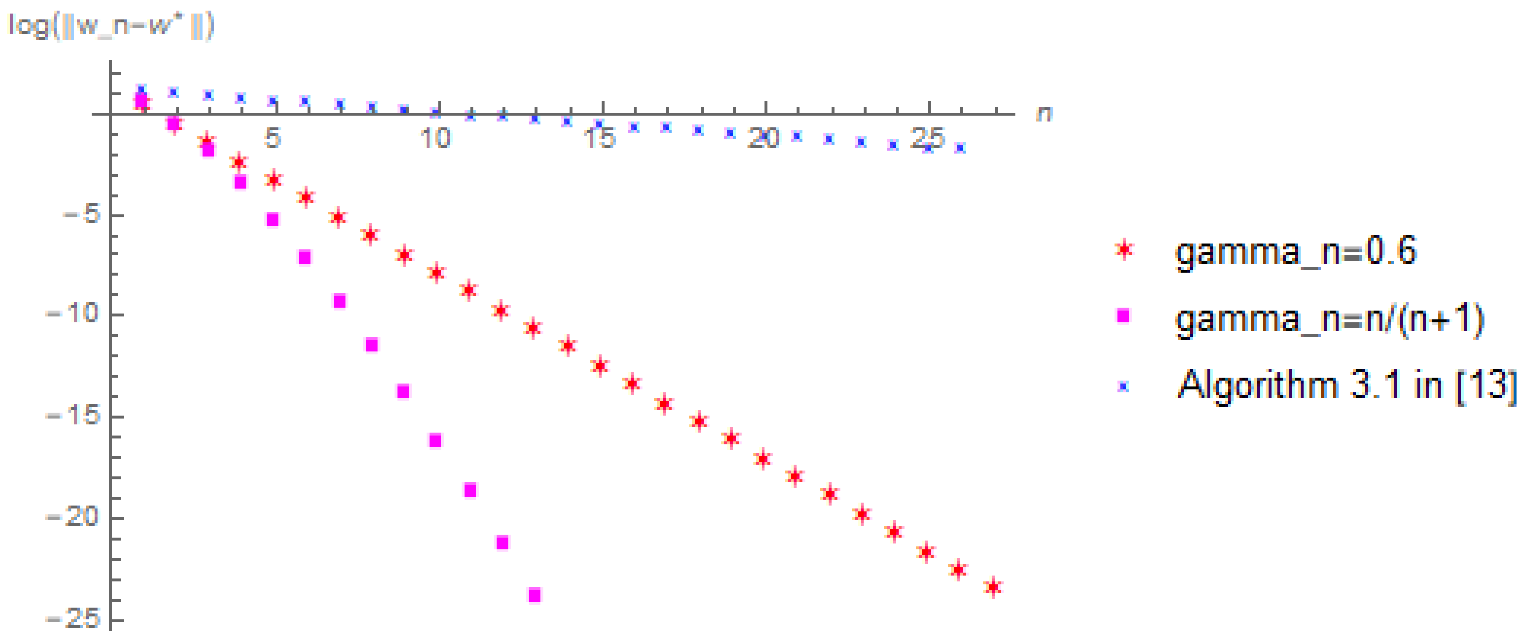
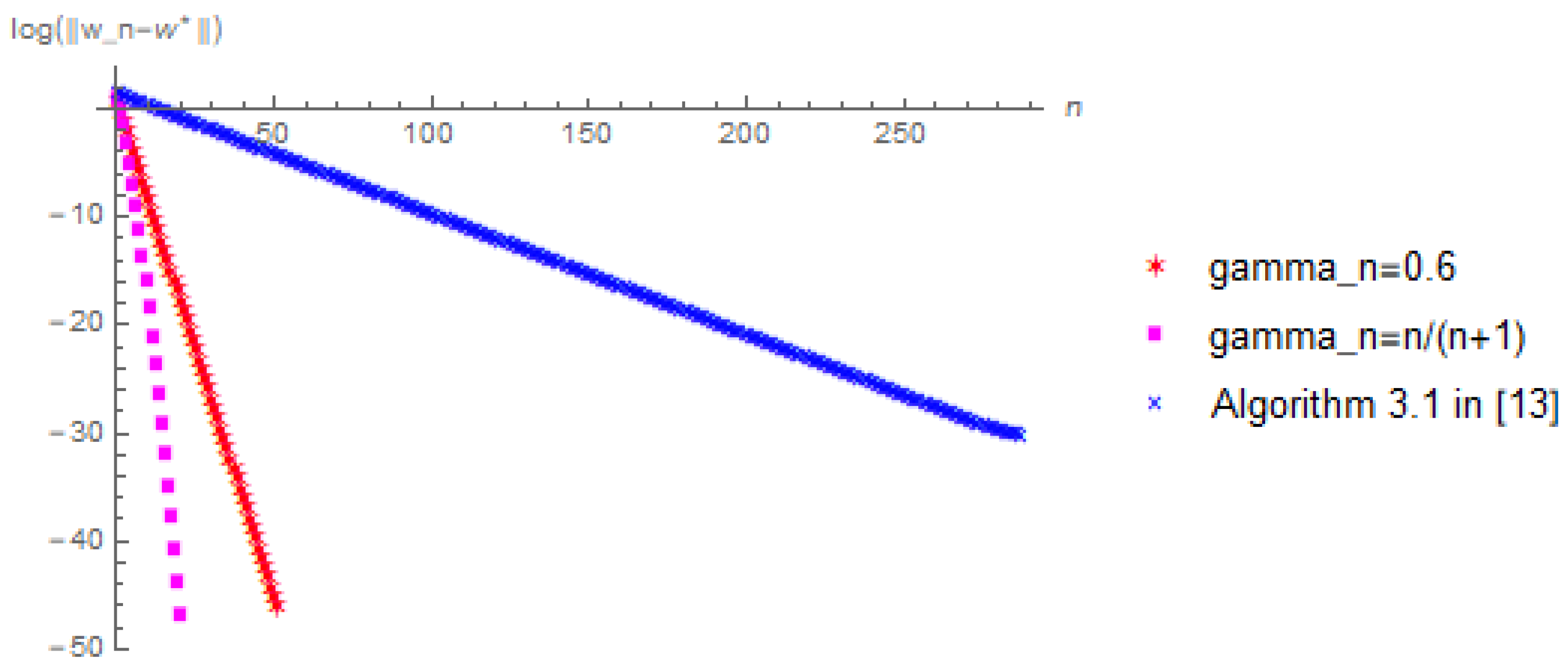
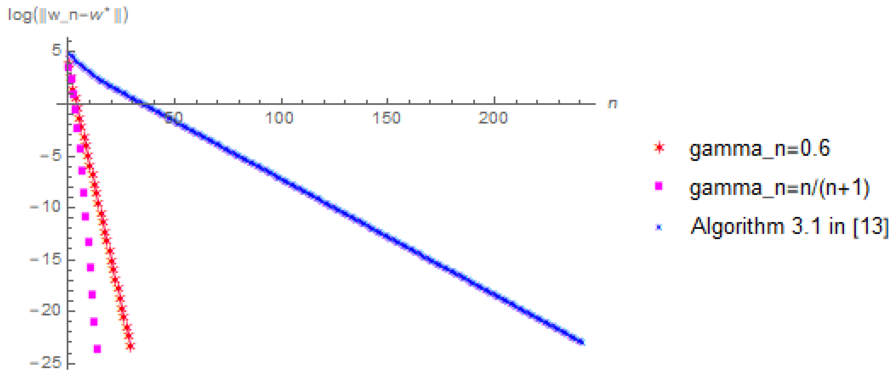
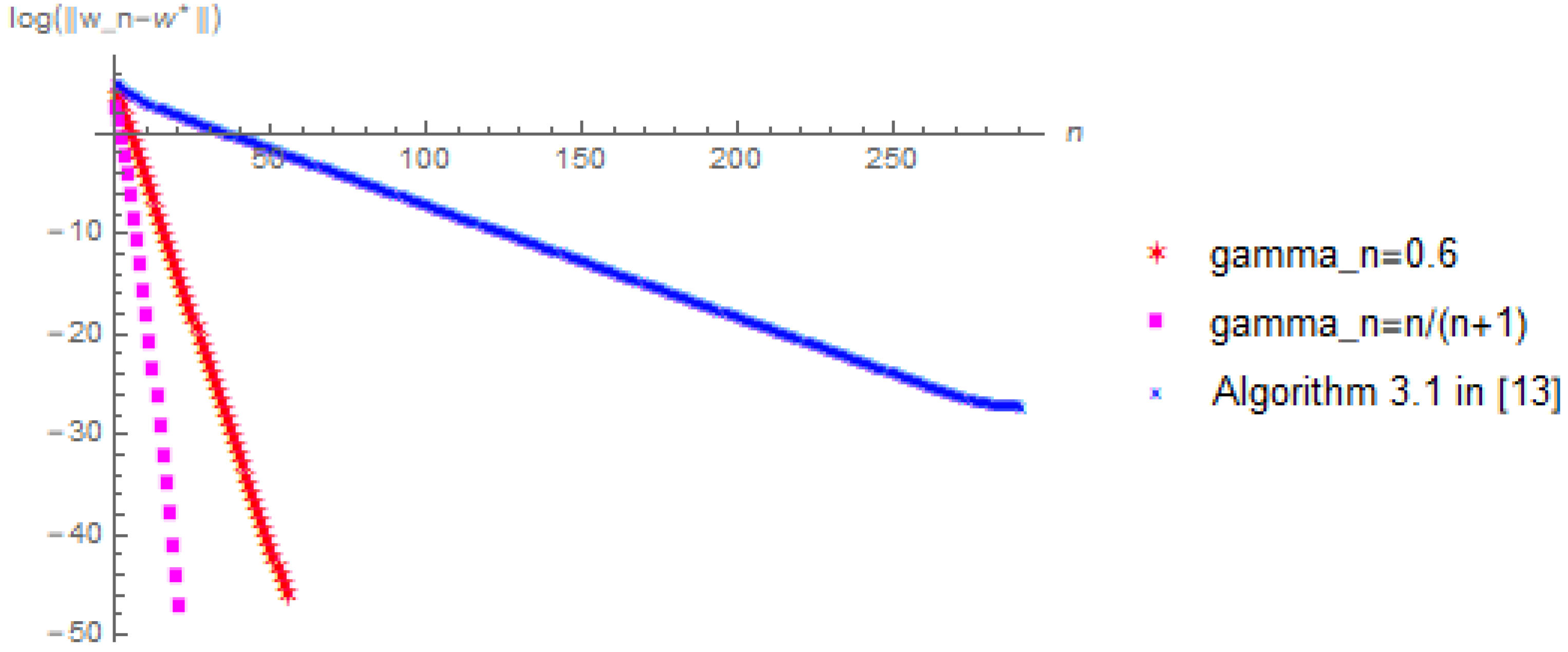
In algorithm (25), we take ${\gamma }_n=0.6,\frac{n}{n+1}$. Moreover, we choose the error to be ${10}^{-10}$ and ${10}^{-20}$ and the initial value to be $w_0=(5,8,3)$ and $w_0=(100,300,50)$, respectively. In addition, under the same conditions, we also compare with Dang’s Algorithm 3.1 in [13] to confirm the effectiveness of our proposed algorithm. For convenience, we choose $s=min\{\frac{\rho \left(G^{*}G\right)}{1+\rho \left(G^{*}G\right)},\frac{1}{1+\rho \left(G^{*}G\right)}\}$ in Dang’s Algorithm 3.1. Then we have the following numerical results displayed in Figure 1, Figure 2, Figure 3 and Figure 4. Note that we denote the number of iterations and the logarithm of the error by using the x-coordinate and the y-coordinate of the figures, respectively. We wrote all the codes in Wolfram Mathematica (version 10.3). All the numerical results were run on a personal Asus computer with AMD A9-9420 RADEON R5, 5 COMPUTE. CORES 2C+3G 3.00 GHz and RAM 8.00 GB.

References

1. Censor, Y.; Elfving, T. A multiprojection algorithm using Bregman projections in a product space. Numer. Algorithms 1994, 8, 221–239. [Google Scholar] [CrossRef]
2. Censor, Y.; Bortfeld, T.; Martin, B. A unified approach for inversion problems in intensity-modulated radiation therapy. Phys. Med. Biol. 2006, 5, 2353–2365. [Google Scholar] [CrossRef] [PubMed]
3. Byrne, C. A unified traetment of some iterative algorithms in signal processing and image reconstruction. Inverse Probl. 2004, 20, 103–120. [Google Scholar] [CrossRef]
4. He, H.; Ling, C.; Xu, H.K. An implementable splitting algorithm for the 1-norm regularized split feasibility problem. J. Sci. Comput. 2015, 67, 1–18. [Google Scholar]
5. Byrne, C. Iterative oblique projection onto convex sets and the split feasibility problem. Inverse Probl. 2002, 18, 441–453. [Google Scholar] [CrossRef]
6. López, G.; Martin-Marquez, V.; Wang, F.; Xu, H.K. Solving the split feasibility problem without prior knowledge of matrix norms. Inverse Probl. 2012, 28, 085004. [Google Scholar]
7. Cegielski, A. Strong convergence of a hybrid steepest descent method for the split common fixed point problem. Optimization 2016, 6, 1463–1476. [Google Scholar] [CrossRef]
8. Yang, Q. The relaxed CQ algorithm solving the split feasibility problem. Inverse Probl. 2004, 20, 1261–1266. [Google Scholar] [CrossRef]
9. Dang, Y.; Gao, Y. The strong convergence of a KM-CQ-like algorithm for a split feasibility problem. Inverse Probl. 2011, 27, 015007. [Google Scholar] [CrossRef]
10. Censor, Y.; Elfving, T.; Kopf, N.; Bortfeld, T. The multiple-sets split feasibility problem and its applications for inverse problems. Inverse Probl. 2005, 21, 2071–2084. [Google Scholar] [CrossRef] [Green Version]
11. Censor, Y.; Motova, A.; Segal, A. Perturbed projections and subgradient projections for the multiple-sets split feasibility problem. J. Math. Anal. Appl. 2007, 327, 1244–1256. [Google Scholar] [CrossRef] [Green Version]
12. Combettes, P.L. Convex set theoretic image reconvery by extrapolated iterations of oarallel subgradient projections. IEEE Trans. Image Process. 1997, 6, 493–506. [Google Scholar] [CrossRef] [PubMed]
13. Dang, Y.Z.; Gao, Y. A new simulitaneous subgradient projection algorithm for solving a multiple-sets split feasibility problem. Appl. Math. 2014, 59, 37–51. [Google Scholar] [CrossRef]
14. Bauschke, H.H.; Combettes, P.L. Convex Analysis and Monotone Operator Theory in Hilbert Spaces; Springer: London, UK, 2011. [Google Scholar]
15. Zhao, X.P.; Ng, K.F.; Li, C.; Yao, J.C. Linear regularity and linear convergence of projection-based methods for solving convex feasibility problems. Appl. Math. Optim. 2018, 78, 613–641. [Google Scholar] [CrossRef]
16. Bauschke, H.H.; Borwein, J.M. On projection algorithms for solving convex feasibility problems. SIAM Rev. 1996, 38, 367–426. [Google Scholar] [CrossRef]
17. Conway, J.B. A Course in Functional Analysis, 2nd ed.; GTM 96; Springer: Berlin/Heidelberg, Germany, 1989. [Google Scholar]
Figure 1. Initial conditions: x 1 = 5 , y 1 = 8 , z 1 = 3 . w * = ( 6.5 , 6.5 , 0 ) , error = 10 10 .
Mathematics 07 00644 g001
Figure 2. Initial conditions: x 1 = 5 , y 1 = 8 , z 1 = 3 . w * = ( 6.5 , 6.5 , 0 ) , error = 10 20 .
Mathematics 07 00644 g002
Figure 3. Initial conditions: x 1 = 100 , y 1 = 300 , z 1 = 50 . w * = ( 200 , 200 , 0 ) , error = 10 10 .
Mathematics 07 00644 g003
Figure 4. Initial conditions: x 1 = 100 , y 1 = 300 , z 1 = 50 . w * = ( 200 , 200 , 0 ) , error = 10 20 .
Mathematics 07 00644 g004