Figure 1.
Two energy groups fluxes for a sphere made of 93% enriched U. Dotted line: Thermal flux, Dashed line: Fast flux, Solid line: Total fluxes.
Figure 1.
Two energy groups fluxes for a sphere made of 93% enriched U. Dotted line: Thermal flux, Dashed line: Fast flux, Solid line: Total fluxes.
Figure 2.
Two energy groups fluxes of a cylinder made of 93% enriched U. Dotted line: Thermal flux, Dashed line: Fast flux, Solid line: Total fluxes.
Figure 2.
Two energy groups fluxes of a cylinder made of 93% enriched U. Dotted line: Thermal flux, Dashed line: Fast flux, Solid line: Total fluxes.
Figure 3.
Two Energy Groups fluxes for an infinite Slab of 93% enriched U. Dotted line: Thermal flux, Dashed line: Fast flux, Solid line: Total fluxes.
Figure 3.
Two Energy Groups fluxes for an infinite Slab of 93% enriched U. Dotted line: Thermal flux, Dashed line: Fast flux, Solid line: Total fluxes.
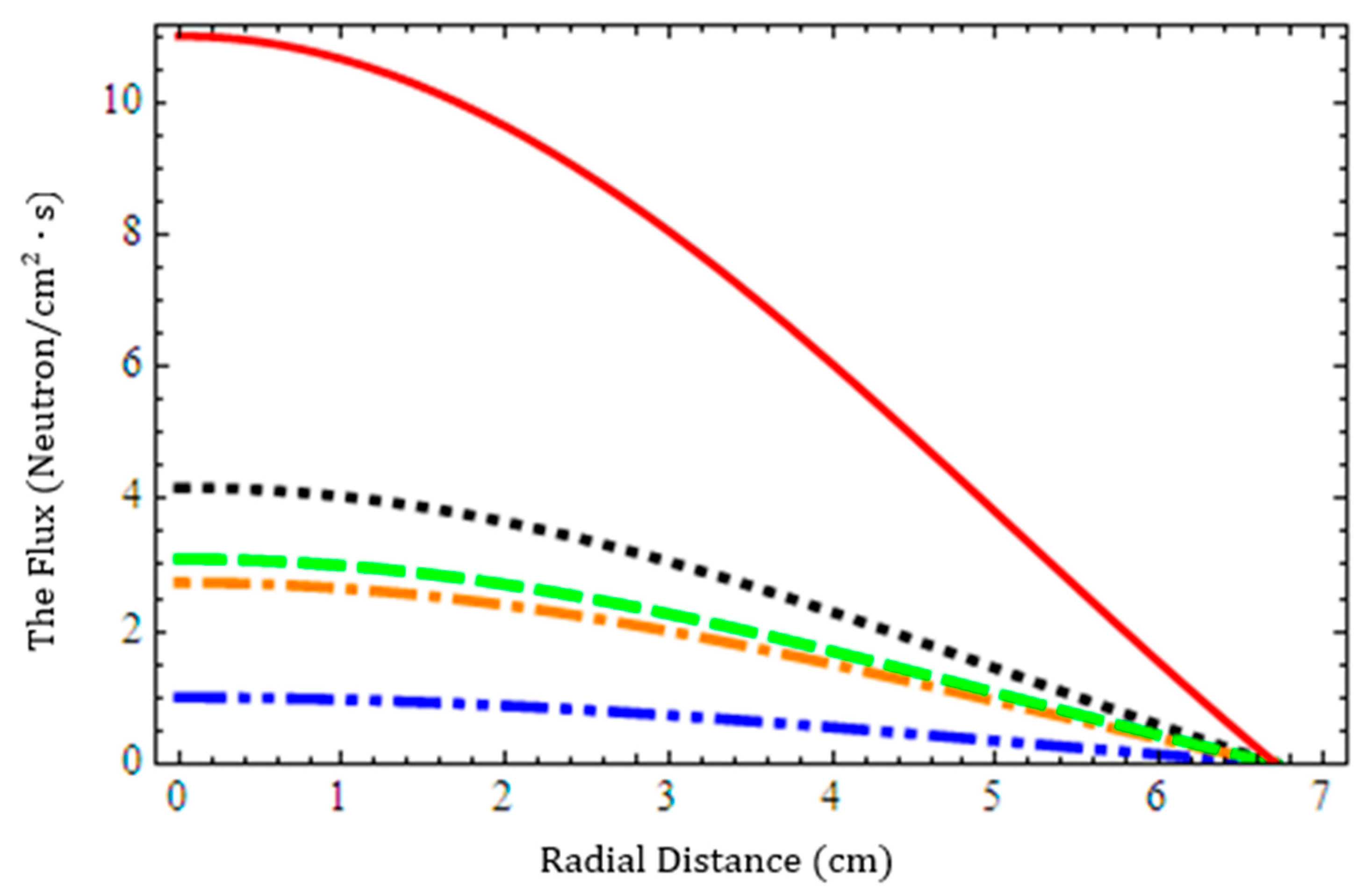
Figure 4.
Four energy groups fluxes and total flux for a spherical reactor. Dotted-dotted dashed line: , Dotted line: , Dotted dashed line: , Dashed line: , Solid line: Total fluxes.
Figure 4.
Four energy groups fluxes and total flux for a spherical reactor. Dotted-dotted dashed line: , Dotted line: , Dotted dashed line: , Dashed line: , Solid line: Total fluxes.
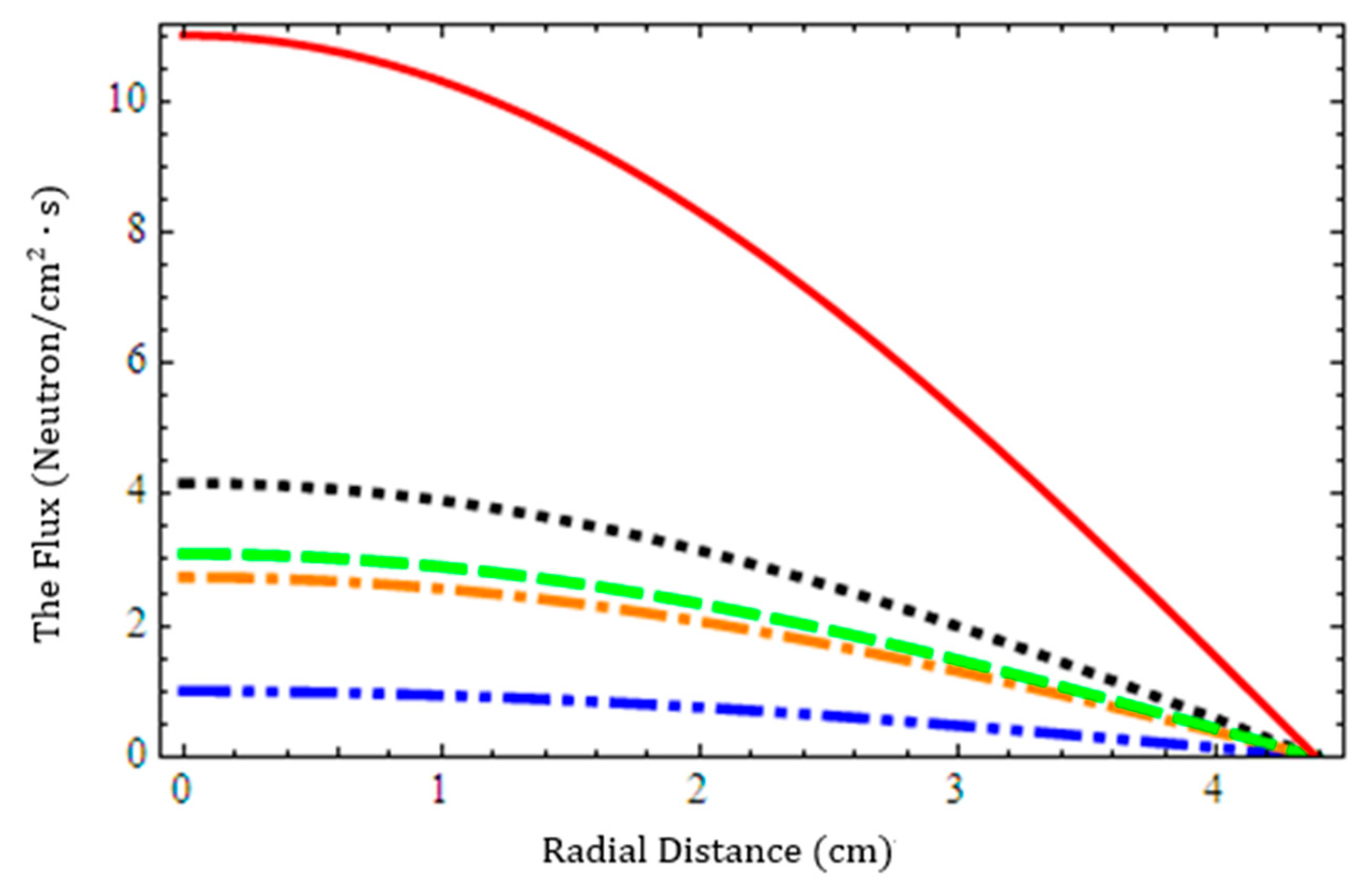
Figure 5.
Four energy groups fluxes and total flux for a cylindrical reactor. Dotted-dotted dashed line: , Dotted line: , Dotted dashed line: , Dashed line: , Solid line: Total fluxes.
Figure 5.
Four energy groups fluxes and total flux for a cylindrical reactor. Dotted-dotted dashed line: , Dotted line: , Dotted dashed line: , Dashed line: , Solid line: Total fluxes.
Figure 6.
Four energy groups fluxes and total flux for a slab reactor. Dotted-dotted dashed line: , Dotted line: , Dotted dashed line: , Dashed line: , Solid line: Total fluxes.
Figure 6.
Four energy groups fluxes and total flux for a slab reactor. Dotted-dotted dashed line: , Dotted line: , Dotted dashed line: , Dashed line: , Solid line: Total fluxes.
Table 1.
Two Group Data.
| Fast Energy Group |
| | |
| | |
| Thermal Energy Group |
| | |
| | |
Table 2.
The values of the coefficients are calculated from Equation (3).
Table 2.
The values of the coefficients are calculated from Equation (3).
| | | |
Table 3.
The critical radius of a 93 % enriched Uranium spherical reactor.
Table 3.
The critical radius of a 93 % enriched Uranium spherical reactor.
| BC | Classical Method | RPSM | Transport Theory |
|---|
| ZF | | | - |
| EBC | | | 16.049836 |
Table 4.
The normalized thermal, fast and total fluxes in a spherical geometry.
Table 4.
The normalized thermal, fast and total fluxes in a spherical geometry.
| Flux | Method | | | | | | |
|---|
| Fast | Classical | | | | | | |
| | RPSM | | | | | | |
| Thermal | Classical | | | | | | |
| | RPSM | | | | | | |
| Total | Classical | | | | | 1.3699 | 0.2498 |
| | RPSM | | | | | 1.3699 | 0.2498 |
Table 5.
The cylindrical reactor critical radius for two boundary conditions
Table 5.
The cylindrical reactor critical radius for two boundary conditions
| BC | Classical Method | RPSM |
|---|
| ZF | | |
| EBC | | |
Table 6.
The normalized thermal, fast, and total fluxes values across a cylindrical geometry.
Table 6.
The normalized thermal, fast, and total fluxes values across a cylindrical geometry.
| Flux | Method | | | | | | |
|---|
| Fast | Classical | | | | | | |
| | RPSM | | | | | | |
| Thermal | Classical | | | | | | |
| | RPSM | | | | | | |
| Total | Classical | | | | | 1.5340 | 0.3213 |
| | RPSM | | | | | 1.5340 | 0.3213 |
Table 7.
The slab reactor critical radius for two boundary conditions.
Table 7.
The slab reactor critical radius for two boundary conditions.
| BC | Classical Method | RPSM | Transport Theory |
|---|
| ZF | | | |
| EBC | | | |
Table 8.
The normalized thermal, fast and total fluxes values across a slab geometry.
Table 8.
The normalized thermal, fast and total fluxes values across a slab geometry.
| Flux | Method | | | | | | |
|---|
| Fast | Transport | | | | | | |
| | Classical | | | | | | |
| | RPSM | | | | | | |
| Thermal | Transport | | | | | | |
| | Classical | | | | | | |
| | RPSM | | | | | | |
| Total | Transport | | | | | | |
| | Classical | | | | | | |
| | RPSM | | | | | | |
Table 9.
Group data.
| Group 1 (1.35 Mev – 10 Mev) |
| | |
| | |
|
| Group 2 (9.1 kev - 1.35 Mev) |
| | |
| | |
|
| Group 3 (0.4 ev – 9.1 kev) |
| | |
| | |
|
| Group 4 (0.0 ev – 0.4 ev) |
| | |
| | |
|
Table 10.
The values of the coefficients.
Table 10.
The values of the coefficients.
| | | |
| | | |
| | | |
| | | |
Table 11.
The spherical reactor critical radius .
Table 11.
The spherical reactor critical radius .
| BC | Classical Method | RPSM |
|---|
| ZF | 8.770 | 8.770 |
| EBC | 7.905 | 7.905 |
Table 12.
The four groups fluxes and total flux in spherical reactor geometry.
Table 12.
The four groups fluxes and total flux in spherical reactor geometry.
| Flux | Method | | | | | | |
|---|
| Group 1 | Classical | | | | | | |
| | RPSM | | | | | | |
| Group 2 | Classical | | 4.1716 | | | | |
| | RPSM | | 4.1716 | | | | |
| Group 3 | Classical | | 2.7361 | | | | |
| | RPSM | | 2.7361 | | | | |
| Group 4 | Classical | | 3.0931 | | | | |
| | RPSM | | 3.0931 | | | | |
| Total | Classical | | 11.0008 | | | | |
| | RPSM | | 11.0008 | | | | |
Table 13.
Cylindrical reactor critical radius for two boundary conditions.
Table 13.
Cylindrical reactor critical radius for two boundary conditions.
| BC | Classical Method | RPSM |
|---|
| ZF | 6.71303 | 6.71303 |
| EBC | 5.84763 | 5.84763 |
Table 14.
The four groups fluxes and total flux in cylindrical reactor geometry.
Table 14.
The four groups fluxes and total flux in cylindrical reactor geometry.
| Flux | Method | | | | | | |
|---|
| Group 1 | Classical | | | 0.9326 | 0.743977 | 0.471824 | 0.169557 |
| | RPSM | | | 0.9326 | 0.743977 | 0.471824 | 0.169557 |
| Group 2 | Classical | | 4.1716 | 3.8904 | 3.10354 | 1.96824 | 0.707317 |
| | RPSM | | 4.1716 | 3.8904 | 3.10354 | 1.96824 | 0.707317 |
| Group 3 | Classical | | 2.7361 | 2.55169 | 2.0356 | 1.29096 | 0.463925 |
| | RPSM | | 2.7361 | 2.55169 | 2.0356 | 1.29096 | 0.463925 |
| Group 4 | Classical | | 3.0931 | 2.88465 | 2.30122 | 1.45941 | 0.524462 |
| | RPSM | | 3.0931 | 2.88465 | 2.30122 | 1.45941 | 0.524462 |
| Total | Classical | | 11.0008 | 10.2593 | 8.18434 | 5.19044 | 1.86526 |
| | RPSM | | 11.0008 | 10.2593 | 8.18434 | 5.19044 | 1.86526 |
Table 15.
The slab reactor critical radius for both boundary conditions.
Table 15.
The slab reactor critical radius for both boundary conditions.
| BC | Classical Method | RPSM |
|---|
| ZF | 4.38485 | 4.38485 |
| EBC | 3.51945 | 3.51945 |
Table 16.
The four groups fluxes and total flux in slab reactor geometry.
Table 16.
The four groups fluxes and total flux in slab reactor geometry.
| Flux | Method | | | | | | |
|---|
| Group 1 | Classical | | | 0.950736 | 0.807797 | 0.585267 | 0.305072 |
| | RPSM | | | 0.950736 | 0.807797 | 0.585267 | 0.305072 |
| Group 2 | Classical | | 4.1716 | 0.950736 | 0.807797 | 0.585267 | 0.305072 |
| | RPSM | | 4.1716 | 0.950736 | 0.807797 | 0.585267 | 0.305072 |
| Group 3 | Classical | | 2.7361 | 2.60131 | 2.21021 | 1.60135 | 0.834709 |
| | RPSM | | 2.7361 | 2.60131 | 2.21021 | 1.60135 | 0.834709 |
| Group 4 | Classical | | 3.0931 | 2.94075 | 2.49862 | 1.81031 | 0.943628 |
| | RPSM | | 3.0931 | 2.94075 | 2.49862 | 1.81031 | 0.943628 |
| Total | Classical | | 11.0008 | 10.4588 | 8.88641 | 6.4384 | 3.35604 |
| | RPSM | | 11.0008 | 10.4588 | 8.88641 | 6.4384 | 3.35604 |
Table 17.
The value of the th-residual error ( for the results obtained by classical method.
Table 17.
The value of the th-residual error ( for the results obtained by classical method.
| | | | |
|---|
| | | | |
| | | | |
| | | | |
| | | | |
| | | | |
| | | | |
Table 18.
The value of the th-residual error ( for the results obtained by RPSM.
Table 18.
The value of the th-residual error ( for the results obtained by RPSM.
| | | | |
|---|
| | | | |
| | | | |
| | | | |
| | | | |
| | | | |
| | | | |


