Total Least Squares Spline Approximation

Abstract

Spline approximation, using both values $y_i$ and $x_i$ as observations, is of vital importance for engineering geodesy, e.g., for approximation of profiles measured with terrestrial laser scanners, because it enables the consideration of arbitrary dispersion matrices for the observations. In the special case of equally weighted and uncorrelated observations, the resulting error vectors are orthogonal to the graph of the spline function and hence can be utilized for deformation monitoring purposes. Based on a functional model that uses cubic polynomials and constraints for continuity, smoothness and continuous curvature, the case of spline approximation with both the values $y_i$ and $x_i$ as observations is considered. In this case, some of the columns of the functional matrix contain observations and are thus subject to random errors. In the literature on mathematics and statistics this case is known as an errors-in-variables (EIV) model for which a so-called “total least squares” (TLS) solution can be computed. If weights for the observations and additional constraints for the unknowns are introduced, a “constrained weighted total least squares” (CWTLS) problem is obtained. In this contribution, it is shown that the solution for this problem can be obtained from a rigorous solution of an iteratively linearized Gauss-Helmert (GH) model. The advantage of this model is that it does not impose any restrictions on the form of the functional relationship between the involved quantities. Furthermore, dispersion matrices can be introduced without limitations, even the consideration of singular ones is possible. Therefore, the iteratively linearized GH model can be regarded as a generalized approach for solving CWTLS problems. Using a numerical example it is demonstrated how the GH model can be applied to obtain a spline approximation with orthogonal error vectors. The error vectors are compared with those derived from two least squares (LS) approaches.

1. Introduction

To capture the geometry of arbitrary objects as completely as possible, nowadays in engineering geodesy areal (area-wise, in contrast to point-wise) measurement methods are applied. Examples are terrestrial laser scanning or photogrammetric approaches based on the evaluation of image data. However, the resulting point cloud is almost never used as a final result since the creation of Computer-aided Design (CAD) models or deformation analyses require a curve or surface approximation by a continuous mathematical function. An overview of curve and surface approximations of three-dimensional (3D) point clouds, including polynomial curves, Bézier curves, B-Spline curves and NURBS curves, was presented by Bureick et al. [1]. Ezhov et al. [2] elaborated the basic methodology of spline approximation in two dimensions (2D) from a geodetic point of view using splines constructed from ordinary polynomials of the form $y_i=f(x_i)$. In the resulting adjustment problem, the values $y_i$ were introduced as observations subject to random errors and the values $x_i$ as error-free values. This approach is relevant, for example, for the following applications:

• Registration of a signal at certain time intervals, whereby the time measurement is much more precise than the measurement of the signal and can therefore be considered as error-free.
• Acquisition of measurements at fixed sensor positions, e.g., measurement of vertical displacements with displacement transducers at fixed horizontal positions during a load test.
• Regarding the values $x_i$ as error-free to generate a solution using a linear functional model. This can be justified when the interpretation of the error vectors (in contrast to deformation analysis) is not the primary aim, but point clouds are approximated to obtain results that primarily satisfy aesthetic requirements.

The fundamental concept and the statistical properties of geodetic measurements are explained e.g., by Mikhail [3] (p. 3 ff.). In that textbook, on page 24, it is pointed out that in practical applications, normal distributions are encountered very often, since in geodesy random variables that represent measurements (respectively, their errors) are often nearly normally distributed. In this contribution we consider the case that both values $y_i$ and $x_i$ of spline functions of the form $y_i=f(x_i)$ are observations subject to random errors. An example for this case is the spline approximation in the field of deformation monitoring where the data were captured with a profile laser scanner.

If the dispersion matrix is a scalar multiple of the identity matrix, the observations $y_i$ and $x_i$ are equally weighted and uncorrelated and a parameter estimation using the method of least squares yields a result where the error vectors of each point are orthogonal to the computed spline approximation. This characteristic is of vital importance for the interpretation of the error vectors not only for the purpose of deformation analysis in engineering geodesy but in many other scientific fields. Hence, a vast literature has been created that discusses the general problem of “orthogonal distance fitting”. Elaborations of this topic are offered e.g., by Sourlier [4], Turner [5] and Ahn [6].

In the contribution of Crambes [7] the case of spline approximation with $y_i$ and $x_i$ as erroneous observations is regarded as errors-in-variables (EIV) model and a total least squares (TLS) solution is presented. A total least squares fitting of Bézier curves to ordered data with an extension to B-spline curves was proposed by Borges and Pastva [8]. They developed an algorithm for applying the Gauss-Newton approach to this problem with a direct method for evaluating the Jacobian based on implicitly differentiating a pseudo-inverse. However, a dispersion matrix for the observations was not introduced.

Jazaeri et al. [9] have presented a new algorithm for solving arbitrary weighted TLS problems within an EIV model having linear and quadratic constraints and singular dispersion matrices. They equivalently translate the weighted total least squares (WTLS) objective function under consideration of the constraints into the Lagrange target function of the constrained minima technique to derive an integrative solution. Fang [10] presented a WTLS and constrained weighted total least squares (CWTLS) solution based on Newton iteration.

In this contribution, we follow the idea of Neitzel [11] and present a total least squares spline approximation as a rigorous evaluation of an iteratively linearized Gauss-Helmert (GH) model taking into account additional constraints for the unknowns. This model has the advantage that it does not impose any restrictions on the form of the functional relationship between the quantities involved in the model. The functional model of 2D similarity transformation discussed by Neitzel [11], e.g., yields a functional matrix that contains two columns that do not contain any random errors (“fixed” or “frozen” columns in the frame of TLS terminology) and two columns in which the same $x$- and $y$-values appear crosswise (one with reversed sign). In order to appropriately consider this structure of the functional matrix, special TLS algorithms must be applied, as presented by Mahboub [12], Schaffrin et al. [13] or Han et al. [14], while this case can be solved in a standard way in the GH model. Furthermore, arbitrary and even singular dispersion matrices can be introduced into the GH model as shown by Schaffrin et al. [15] and Neitzel and Schaffrin [16]. Therefore, the iteratively linearized GH model can be regarded as a generalized approach for solving constrained weighted total least squares (CWTLS) problems.

The aim of this publication is not to investigate which algorithm is more efficient, but rather to show that the TLS spline approximation can be solved in the well-known GH model, which can be traced back to Helmert [17] (p. 285 ff.), and to offer the algorithm which can be used for solving practical geodetic problems.

2. A Review of the Errors-in-Variables (EIV) Model

Using the function of a cubic polynomial as an example, a brief overview of the errors-in-variables (EIV) model with regular dispersion matrix is presented in the following. In the case of the EIV model with a singular dispersion matrix, please refer to the contribution of Schaffrin et al. [15]. Ezhov et al. [2] elaborated a spline function constructed from ordinary cubic polynomials

$$y_i=a_0+a_1{x}_i+a_2{x}_i^2+a_3{x}_i^3$$

(1)

with additional constraints to impose continuity, smoothness and continuous curvature. Under consideration of the values $y_i$ as observations subject to random errors $e_{y_i}$, values $x_i$ as fixed (error-free) values and $a_0,a_1,a_2,a_3$ as unknowns, the observation equations

$$y_i-e_{y_i}={\widehat{a}}_0+{\widehat{a}}_1{x}_i+{\widehat{a}}_2{x}_i^2+{\widehat{a}}_3{x}_i^3$$

(2)

are obtained. For a description of the constraint equations please refer to Ezhov et al. [2]. The resulting adjustment problem can be expressed as

$$L-e_L=A\widehat{X},$$

(3)

$$e_L\sim (0,\hspace{0.17em}{\sigma }_0^2{Q}_{LL}),$$

(4)

$$c=C\widehat{X},$$

(5)

where

• $L$ is the observation vector containing the values $y_i$,
• $e_L$ the normally distributed random error vector associated with $L$ containing the values $e_{y_i}$ with expected value $0$ and dispersion matrix $Q_{LL}$,
• $A$ the functional matrix containing the coefficients $1,\hspace{0.17em}{x}_i,\hspace{0.17em}{x}_i^2,\hspace{0.17em}{x}_i^3$ of the linear functional model,
• $\widehat{X}$ the vector of adjusted unknowns containing the parameters ${\widehat{a}}_{0_j},\hspace{0.17em}{\widehat{a}}_{1_j},\hspace{0.17em}{\widehat{a}}_{2_j},\hspace{0.17em}{\widehat{a}}_{3_j}$,
• $c$ the vector with given constant values,
• $C$ the functional matrix containing the coefficients of the linear constraints for the unknowns, refer to Ezhov et al. [2] for details, and
• ${\sigma }_0^2$ the theoretical reference standard deviation.

With $Q_{LL}$ being a non-singular matrix the corresponding weight matrix can be computed from

$$P=Q_{LL}^{-1}.$$

(6)

Introducing the vector $\mathsf{\lambda }$ of Lagrange multipliers, the constrained minima technique can be applied which yields the objective function

$$\mathsf{\Phi }(e_L,\mathsf{\lambda },\widehat{X})=e_L^{\mathrm{T}}P\hspace{0.17em}{e}_L+2{\mathsf{\lambda }}^{\mathrm{T}}(C\widehat{X}-c)=\min ,$$

(7)

compare with the textbook by Mikhail [3] (p. 215). The solution can be obtained from a Gauss-Markov (GM) model with constraints, as shown in detail by Ezhov et al. [2].

If we now consider both the values $y_i$ and the values $x_i$ as observations, we have to introduce not only errors $e_{y_i}$ associated with the values $y_i$ but also errors $e_{x_i}$ associated with observations $x_i$ and we obtain the condition equations

$$y_i-e_{y_i}={\widehat{a}}_0+{\widehat{a}}_1(x_i-e_{x_i})+{\widehat{a}}_2{(x_i-e_{x_i})}^2+{\widehat{a}}_3{(x_i-e_{x_i})}^3.$$

(8)

For a description of the additional constraint equations please refer to Ezhov et al. [2]. Starting from (3) these condition equations can be expressed in a general form as a so-called errors-in-variables (EIV) model (in which some of the columns of the functional matrix $A$ contain observations and are thus subject to random errors $E_A$) with constraints

$$L-e_L=(A-E_A)\widehat{X},$$

(9)

$$c=C\widehat{X}.$$

(10)

The normally distributed random error vector associated with $L$ and $A$ containing the vectors $e_L$ and $e_A$ with expected value ${[\begin{array}{cc}0& 0\end{array}]}^{\mathrm{T}}$ and dispersion matrix $Q$ reads

$$\left[\begin{array}{c}{e}_L\\ e_A\end{array}\right]=\left[\begin{array}{c}{e}_L\\ \mathrm{vec}\hspace{0.17em}{E}_A\end{array}\right]\sim (\left[\begin{array}{c}0\\ 0\end{array}\right],\hspace{0.17em}{\sigma }_0^{2}Q={\sigma }_0^2\left[\begin{array}{cc}{Q}_{LL}& Q_{LA}\\ Q_{AL}& Q_{AA}\end{array}\right]),$$

(11)

where

• $E_A$ is the random error matrix associated with $A$ containing the values $e_{x_i}$, and
• $e_A$ the vectorized form of $E_A$.

From the non-singular dispersion matrix $Q$, the weight matrix

$$P=Q^{-1}=\left[\begin{array}{cc}{P}_{11}& P_{12}\\ P_{21}& P_{22}\end{array}\right]$$

(12)

can be computed, which leads to the objective function

$$\mathsf{\Phi }(e_L,e_A,\mathsf{\lambda },\widehat{X})=\left[\begin{array}{cc}{e}_L^{\mathrm{T}}& e_A^{\mathrm{T}}\end{array}\right]\hspace{0.17em}\left[\begin{array}{cc}{P}_{11}& P_{12}\\ P_{21}& P_{22}\end{array}\right]\hspace{0.17em}\left[\begin{array}{c}{e}_L\\ e_A\end{array}\right]+2{\mathsf{\lambda }}^{\mathrm{T}}(C\widehat{X}-c)=\min .$$

(13)

The solution for this EIV model can be determined (amongst others) using the TLS approach, more precisely in this case the constrained weighted total-least squares (CWTLS) approach. The notion “total least squares” (TLS) was introduced by Golub and van Loan [18] and very elegant solution algorithms based on singular value decomposition (SVD) were developed; see, e.g., the contributions by Golub and van Loan [18], van Huffel and Vandewalle [19] (p. 29 ff.) or Markovsky and van Huffel [20].

However, a solution with SVD is only possible if the functional model of the adjustment problem is pseudo-linear and if it has a certain structure, yielding a functional matrix that does not contain fixed (error-free) columns or columns in which the same variables occur multiple times (e.g., crosswise). The problem discussed in this article does not belong to this class. A systematic approach for direct solutions of specific non-linear adjustment problems such as fitting of a straight line in 2D and 3D, fitting of a plane in 3D and 2D similarity transformation with all coordinates introduced as observations subject to random errors was elaborated from a geodetic point of view by Malissiovas et al. [21].

Jazaeri et al. [9] have presented a new flexible algorithm for solving the weighted TLS problem within an EIV model having linear and quadratic constraints and singular dispersion matrices. Their iterative algorithm is based on an equivalent translation of the objective function (13) subject to (9) and (10) into a Lagrange target function. The case of quadratic constraints occurs, e.g., when the 2D or 3D coordinate transformation is formulated for the most general case (affine transformation) and the cases of similarity or rigid transformation are imposed with the help of constraint equations, which was shown by Fang [10]. Singular dispersion matrices are always associated with coordinates computed from a free network adjustment, as explained by Neitzel and Schaffrin [16].

The term errors-in-variables (EIV) model was introduced in the literature on mathematics and statistics. It is used for regression models where measurement errors are taken into account for both, the dependent variables and the independent variables. For geodesists, this terminology is rather confusing, because whenever we introduce errors, they are inherently associated with the term observations and not with variables. A remark of this kind was also given by Fuller [22], who explained: “The term errors in variables is used in econometrics, while the terms observation error or measurement error are common in other areas of statistical application.” Thus, it is immediately evident that an EIV model is just another formulation of a well-known adjustment problem. Therefore, we can rearrange the EIV model (8) and obtain an implicit form of the functional relation

$$y_i-e_{y_i}-{\widehat{a}}_0-{\widehat{a}}_1(x_i-e_{x_i})-{\widehat{a}}_2{(x_i-e_{x_i})}^2-{\widehat{a}}_3{(x_i-e_{x_i})}^3=0,$$

(14)

which is an example of a functional relationship that leads to the adjustment of (nonlinear) condition equations with unknowns that can already be found in the classical textbook of Helmert [17] (p. 285 ff.).

Neitzel [11] showed using the example of unweighted and weighted 2D similarity transformation that the TLS solution within an EIV model can be obtained from a rigorous solution of an iteratively linearized Gauss-Helmert model. After the definition of a spline constructed from ordinary cubic polynomials in Section 3 and the definition of the problem in Section 4, we will follow this idea and show in Section 5 how to derive the constrained weighted total-least squares (CWTLS) of an EIV model from a rigorous solution of an iteratively linearized Gauss-Helmert model with additional constraints for the unknowns. A numerical example will be presented in Section 6 followed by conclusions and outlook in Section 7.

3. Definition of a Spline Constructed from Ordinary Cubic Polynomials

For the definition of a spline constructed from ordinary cubic polynomials the elaboration from Ezhov et al. [2] is presented in what follows. Considering a 2D Cartesian coordinate system, Figure 1 illustrates a spline interpolation where the given knots are interpolated by a piecewise continuous spline consisting of polynomials which meet at these knots. The coordinates of the knots are denoted by $(x_{k_j},y_{k_j})$; hence, $j=0,1,\dots ,n$ is the index (ordinal number) of the knot and $n$ the number of segments. Character $k$ stands for “knot” and is not an index; hence, $x_{k_j}$ means “$x$-value of the knot $j$”. Then the spline is given by the function $S(x)$ with the following properties:

• $S(x)$ is a piecewise cubic polynomial with knots at $x_{k_0}$, $x_{k_1}$, …, $x_{k_n}$,
• $S(x)$ is a linear polynomial for $x\le x_{k_0}$ and $x\ge x_{k_n}$,
• $S(x)$ has two continuous derivatives everywhere,
• $S(x_{k_j})=y_{k_j}$ for $j=0,1,\dots ,n$.

According to Schumaker [23] (p. 7) $S(x)$ (see Figure 1) defined as above, is in a way the best interpolating function. This is one of the reasons why the cubic spline is generally accepted as the most relevant of all splines.

Starting from the above mentioned properties a spline function can be defined as

$$S(x)=\{\begin{array}{cc}{S}_1(x),& x_{k_0}\le x\le x_{k_1}\\ ⋮& \\ S_j(x),& x_{k_{j-1}}\le x\le x_{k_j}\\ ⋮& \\ S_n(x),& x_{k_{n-1}}\le x\le x_{k_n}\end{array},$$

(15)

where the expression for a cubic polynomial in each segment $j$ can be written as

$$S_j(x)=a_{0_j}+a_{1_j}x+a_{2_j}{x}^2+a_{3_j}{x}^3,\hspace{1em}j=1,2,\dots ,n.$$

(16)

The property that the spline has to meet exactly the data at the given knots yields the conditions

$$S_j(x_{k_{j-1}})=y_{k_{j-1}} \mathrm{and} S_j(x_{k_j})=y_{k_j},\hspace{1em}j=1,2,\dots ,n.$$

(17)

The property that $S(x)$ has two continuous derivatives everywhere yields the constraints

$$S_j^{\prime }(x_{k_j})=S_{j+1}^{\prime }(x_{k_j}),\hspace{1em}j=1,2,\dots ,n-1,$$

(18)

$$S_j^{″}(x_{k_j})=S_{j+1}^{″}(x_{k_j}),\hspace{1em}j=1,2,\dots ,n-1.$$

(19)

From Equation (16) and Figure 1 we see that there are $n$ polynomial functions $S_j(x)$ and $n+1$ knots. The cubic function depends on four parameters, and consequently, the spline $S(x)$ on $4n$ unknowns. From (17), we obtain $2n$ and from (18) and (19) we get $2(n-1)$ condition equations. This results in $4n-2$ condition equations to be solved for $4n$ unknowns and hence the equation system is underdetermined. To overcome this problem, arbitrary additional conditions can be introduced. Usually the missing constraints are introduced at the first and the last knot. For more details refer to Ezhov et al. [2].

The main application of spline interpolation is the construction of curves through a sparse sequence of data points, e.g., in the construction of aesthetically pleasing curves in CAD models. The aim is different when modern sensors such as laser scanners are used with an acquisition rate of up to 2 million points per second, providing a very dense sequence of data points. Due to the high point density and the fact that measurements are affected by random errors, it is no longer appropriate to apply spline interpolation, since observation errors and other abrupt changes in the data points would be modeled, resulting in a strongly oscillating spline.

To avoid this effect, the point sequence is divided into not so many intervals using predefined knots. Due to the high point density, this results in an overdetermined configuration and the parameters of piecewise cubic splines can be determined using least squares adjustment. Conditions for smoothness at the knots (where two polynomials meet) can be introduced as constraint equations into the formulation of the adjustment problem. The result is a spline that no longer follows all data points exactly, but as closely as possible, subject to a predefined target function. In the case of least squares adjustment, this means that the sum of the weighted squared residuals becomes minimal. This case, illustrated in Figure 2, is called spline approximation.

For formulating this approximation problem, cubic polynomials (16) are used for each interval of the spline. Furthermore, constraint equations for continuity (17), smoothness (18) and continuous curvature (19) are to be introduced at the knots. Both the values $y_i$ and the values $x_i$ are regarded as observations subject to random errors. An example for this case is the spline approximation in the field of deformation monitoring where the data were captured with a profile laser scanner.

In spline approximation, the parameters for an overdetermined configuration are determined by a least squares adjustment. In contrast to spline interpolation, a solution can be found by minimizing the sum of the weighted squared residuals without imposing any extra conditions to the first and last point of the spline. Only the already mentioned conditions for continuity, smoothness and continuous curvature have to be introduced at the “inner” knots as additional constraints. In the following section the resulting adjustment problem is defined.

4. Definition of the Problem

Let:

• $(x_{1_j},y_{1_j}),\hspace{0.17em}(x_{2_j},y_{2_j}),\hspace{0.17em}\dots ,\hspace{0.17em}(x_{i_j},y_{i_j}),\hspace{0.17em}\dots ,(x_{m_j},y_{m_j})$ be pairs of observed values within an interval $j$, where the sequence on the $x$-axis $x_{1_j}<x_{2_j}<\dots <x_{i_j}<\dots x_{m_j}$ is non-decreasing,
• $\left[\begin{array}{c}{e}_x\\ e_y\end{array}\right]\sim (\left[\begin{array}{c}0\\ 0\end{array}\right],\hspace{0.17em}{\sigma }_0^2{Q}_{LL}={\sigma }_0^2\left[\begin{array}{cc}{Q}_{xx}& Q_{xy}\\ Q_{yx}& Q_{yy}\end{array}\right])$ be the stochastic model and $P=Q_{LL}^{-1}$ the corresponding weight matrix,
• $x_{k_1}<x_{k_2}<\dots <x_{k_j}<\dots <x_{k_{n-1}}$ be a non-decreasing sequence of user-defined values for the knots on the $x$-axis which are regarded as error-free. As mentioned before, the first knot $x_{k_0}$ and the last knot $x_{k_n}$, see Figure 1, have no particular influence on the adjustment, they are just $x_{k_0}=x_{\min }$ and $x_{k_n}=x_{\max }$. Therefore, when the positioning of the knots is discussed, we refer only to the knots $x_{k_1},\dots ,x_{k_j},\dots ,x_{k_{n-1}}$, see Figure 2, on which some constraints are imposed. The positioning of the knots plays a key role in spline approximation problems. This problem is further discussed in Section 5.4.

To determine:

• $(a_{0_1},a_{1_1},a_{2_1},a_{3_1}),\dots ,(a_{0_j},a_{1_j},a_{2_j},a_{3_j}),\dots ,(a_{0_n},a_{1_n},a_{2_n},a_{3_n})$, which represent a set of parameters for the cubic polynomials $S_j(x)$ which has to be estimated for all intervals $[x_{k_{j-1}},x_{k_j})$.

According to (16) the functional model for the cubic polynomials reads

$$y_{i_j}=S_j(x_{i_j})=a_{0_j}+a_{1_j}{x}_{i_j}+a_{2_j}{x}_{i_j}^2+a_{3_j}{x}_{i_j}^3$$

(20)

with $j=1,2,\dots ,n$ as index for an interval $[x_{k_{j-1}},x_{k_j})$. Furthermore, $i=1,2,\dots ,m_j$ represents an index for all pairs of observed values within the interval $j$.

Since an overdetermined system of equations is considered, a spline approximation is performed without putting any extra conditions on the first and the last knots of the spline. The dataset is subdivided into intervals w.r.t. the $x$-axis by predefined knots. For each interval $[x_{k_{j-1}},x_{k_j})$ there is a set of at least two pairs of values $(x_{i_j},y_{i_j})$ inside of it. According to (17)–(19) the conditions

$$S_j(x_{k_j})=S_{j+1}(x_{k_j}),\hspace{1em}j=1,\dots ,n-1$$

(21)

$$S_j^{\prime }(x_{k_j})=S_{j+1}^{\prime }(x_{k_j}),\hspace{1em}j=1,\dots ,n-1$$

(22)

$$S_j^{″}(x_{k_j})=S_{j+1}^{″}(x_{k_j}),\hspace{1em}j=1,\dots ,n-1$$

(23)

are imposed on the knots for constructing a spline. These knots $x_{k_j}$ are also coordinates on the $x$-axis but their number and their values are freely specified, or can be determined by some knot placement strategy, see Section 5.4.

After having defined all these quantities, a spline approximation can be performed from an overdetermined configuration using the Gauss-Helmert model with additional constraints for the unknowns.

5. TLS Solution Generated by Least Squares Adjustment within the Gauss-Helmert Model

In this section, the solution for the weighted total least-squares problem with constraints (CWTLS) (13) is based on “classical” procedures, specifically on an iterative evaluation of the nonlinear normal equations derived for nonlinear condition and constraint equations by least squares adjustment. A common approach does replace the original nonlinear condition and constraint equations by a sequence of linearized equations which obviously requires a correct linearization of the condition and constraint equations. This means that the linearization has to be done both at the approximate values $X^0$ for the unknowns, and at approximate values $e^0$ for the random errors. Such an iterative solution is regarded as “rigorous” evaluation of the iteratively linearized Gauss-Helmert model.

An extensive presentation of an evaluation of this kind was already given e.g., by Pope [24]. Lenzmann and Lenzmann [25] pick up this problem once more and present another rigorous solution for the iteratively linearized GH model. In doing so, they show very clearly which terms when neglected will produce merely approximate formulas. Unfortunately, these approximate formulas, which can yield an unusable solution, can be found in many popular textbooks on adjustment calculus. For more details please refer to Neitzel [11]. The rigorous solution as presented in the following is based on Lenzmann and Lenzmann [25].

5.1. Formulation of the Adjustment Problem

Based on the functional model (20) with observations $y_i$ and $x_i$, the condition equations

$${\psi }_i(e,\widehat{X})=y_i-e_{y_i}-{\widehat{a}}_{0_j}-{\widehat{a}}_{1_j}(x_i-e_{x_i})-{\widehat{a}}_{2_j}{(x_i-e_{x_i})}^2-{\widehat{a}}_{3_j}{(x_i-e_{x_i})}^3=0$$

(24)

can be formulated. Obviously, (24) is nonlinear. However, the application of least squares adjustment usually “lives” in the linear world. Since the Gauss-Newton method is used here for solving least squares problems, the condition equations have to be linearized. With appropriate approximate values $e^0$ and $X^0$, the linearized condition equations can be written as

$$f(e,\hspace{0.17em}\widehat{X})=B(e-e^0)+A(\widehat{X}-X^0)+\mathsf{\psi }(e^0,\hspace{0.17em}{X}^0)=c_1$$

(25)

with $c_1=0$ and the matrices of partial derivatives

$$A(e,\hspace{0.17em}\widehat{X})={\frac{\partial \mathsf{\psi }(e,\hspace{0.17em}\widehat{X})}{\partial \widehat{X}}|}_{e^0,\hspace{0.17em}{X}^0},$$

(26)

$$B(e,\hspace{0.17em}\widehat{X})={\frac{\partial \mathsf{\psi }(e,\hspace{0.17em}\widehat{X})}{\partial e}|}_{e^0,\hspace{0.17em}{X}^0}.$$

(27)

These derivatives have to be evaluated at the approximate values $e^0$ and $X^0$. Taking the partial derivatives for the function that defines the condition Equation (24) with respect to the unknowns

$${\frac{\partial {\psi }_i(e,\hspace{0.17em}\widehat{X})}{\partial {\widehat{a}}_{0_j}}|}_{e^0,X^0}=-1,$$

(28)

$${\frac{\partial {\psi }_i(e,\hspace{0.17em}\widehat{X})}{\partial {\widehat{a}}_{1_j}}|}_{e^0,X^0}=-(x_i-e_{x_i}^0),$$

(29)

$${\frac{\partial {\psi }_i(e,\hspace{0.17em}\widehat{X})}{\partial {\widehat{a}}_{2_j}}|}_{e^0,X^0}=-{(x_i-e_{x_i}^0)}^2,$$

(30)

$${\frac{\partial {\psi }_i(e,\hspace{0.17em}\widehat{X})}{\partial {\widehat{a}}_{3_j}}|}_{e^0,X^0}=-{(x_i-e_{x_i}^0)}^3,$$

(31)

we can set up the matrices $A_j$ for each polynomial piece of the spline. The functional matrix for the first interval reads

$$A_1=-\left[\begin{array}{cccc}1& (x_{1_1}-e_{x_{1_1}}^0)& {(x_{1_1}-e_{x_{1_1}}^0)}^2& {(x_{1_1}-e_{x_{1_1}}^0)}^3\\ 1& (x_{2_1}-e_{x_{2_1}}^0)& {(x_{2_1}-e_{x_{2_1}}^0)}^2& {(x_{2_1}-e_{x_{2_1}}^0)}^3\\ ⋮& ⋮& ⋮& ⋮\\ 1& (x_{m_1}-e_{x_{m_1}}^0)& {(x_{m_1}-e_{x_{m_1}}^0)}^2& {(x_{m_1}-e_{x_{m_1}}^0)}^3\end{array}\right],$$

(32)

for the second interval, we obtain

$$A_2=-\left[\begin{array}{cccc}1& (x_{1_2}-e_{x_{1_2}}^0)& {(x_{1_2}-e_{x_{1_2}}^0)}^2& {(x_{1_2}-e_{x_{1_2}}^0)}^3\\ 1& (x_{2_2}-e_{x_{2_2}}^0)& {(x_{2_2}-e_{x_{2_2}}^0)}^2& {(x_{2_2}-e_{x_{2_2}}^0)}^3\\ ⋮& ⋮& ⋮& ⋮\\ 1& (x_{m_2}-e_{x_{m_2}}^0)& {(x_{m_2}-e_{x_{m_2}}^0)}^2& {(x_{m_2}-e_{x_{m_2}}^0)}^3\end{array}\right].$$

(33)

This construction of $A_j$ matrices continues until the last interval. Finally, the entire functional matrix has the following form

$$A=diag\left[\begin{array}{ccc}{A}_1& \cdots & A_n\end{array}\right].$$

(34)

From (32) and (33), we can see the typical characteristic of an EIV model (9), where some (or sometimes all) columns of the functional matrix contain observations with their corresponding errors.

Taking the partial derivatives of the function $\psi$ from condition Equations (24) with respect to the errors

$${\frac{\partial {\psi }_i(e,\widehat{X})}{\partial e_{x_i}}|}_{e^0,X^0}=a_{1_j}^0+2a_{2_j}^0(x_i-e_{x_i}^0)+3a_{3_j}^0{(x_i-e_{x_i}^0)}^2,$$

(35)

$${\frac{\partial {\psi }_i(e,\hspace{0.17em}\widehat{X})}{\partial e_{y_i}}|}_{e^0,X^0}=-1,$$

(36)

we can define the matrices $B_1$ and $B_2$

$$B_1=diag\left[\begin{array}{ccc}\cdots & a_{1_j}^0+2a_{2_j}^0(x_i-e_{x_i}^0)+3a_{3_j}^0{(x_i-e_{x_i}^0)}^2& \cdots \end{array}\right],$$

(37)

$$B_2=-I.$$

(38)

Finally, matrix $B$ obtains the following form

$$B=\left[\begin{array}{cc}{B}_1& B_2\end{array}\right].$$

(39)

Now, we have to take into account also the constraints (21)–(23). Since the knots $x_k$ are error-free values, we obtain linear constraint equations

$$\begin{array}{ccc}\hfill {\widehat{a}}_{0_1}+{\widehat{a}}_{1_1}{x}_{k_1}+{\widehat{a}}_{2_1}{x}_{k_1}^2+{\widehat{a}}_{3_1}{x}_{k_1}^3& =& {\widehat{a}}_{0_2}+{\widehat{a}}_{1_2}{x}_{k_1}+{\widehat{a}}_{2_2}{x}_{k_1}^2+{\widehat{a}}_{3_2}{x}_{k_1}^3,\hfill \\ \hfill {\widehat{a}}_{0_2}+{\widehat{a}}_{1_2}{x}_{k_2}+{\widehat{a}}_{2_2}{x}_{k_2}^2+{\widehat{a}}_{3_2}{x}_{k_2}^3& =& {\widehat{a}}_{0_3}+{\widehat{a}}_{1_3}{x}_{k_2}+{\widehat{a}}_{2_3}{x}_{k_2}^2+{\widehat{a}}_{3_3}{x}_{k_2}^3,\hfill \\ & ⋮& \\ \hfill {\widehat{a}}_{0_{n-1}}+{\widehat{a}}_{1_{n-1}}{x}_{k_{n-1}}+{\widehat{a}}_{2_{n-1}}{x}_{k_{n-1}}^2+{\widehat{a}}_{3_{n-1}}{x}_{k_{n-1}}^3& =& {\widehat{a}}_{0_n}+{\widehat{a}}_{1_n}{x}_{k_{n-1}}+{\widehat{a}}_{2_n}{x}_{k_{n-1}}^2+{\widehat{a}}_{3_n}{x}_{k_{n-1}}^3\hfill \end{array}$$

(40)

which enforce the spline to be continuous at the knots. The next set of constraint equations

$$\begin{array}{ccc}\hfill {\widehat{a}}_{1_1}+2{\widehat{a}}_{2_1}{x}_{k_1}+3{\widehat{a}}_{3_1}{x}_{k_1}^2& =& {\widehat{a}}_{1_2}+2{\widehat{a}}_{2_2}{x}_{k_1}+3{\widehat{a}}_{3_2}{x}_{k_1}^2,\hfill \\ \hfill {\widehat{a}}_{1_2}+2{\widehat{a}}_{2_2}{x}_{k_2}+3{\widehat{a}}_{3_2}{x}_{k_2}^2& =& {\widehat{a}}_{1_3}+2{\widehat{a}}_{2_3}{x}_{k_2}+3{\widehat{a}}_{3_3}{x}_{k_2}^2,\hfill \\ & ⋮& \\ \hfill {\widehat{a}}_{1_{n-1}}+2{\widehat{a}}_{2_{n-1}}{x}_{k_{n-1}}+3{\widehat{a}}_{3_{n-1}}{x}_{k_{n-1}}^2& =& {\widehat{a}}_{1_n}+2{\widehat{a}}_{2_n}{x}_{k_{n-1}}+3{\widehat{a}}_{3_n}{x}_{k_{n-1}}^2\hfill \end{array}$$

(41)

enforces the spline to have a continuous first derivative at the knots. This implies that the spline will have smooth transition at the knots. The last set of constraint equations

$$\begin{array}{ccc}\hfill 2{\widehat{a}}_{2_1}+6{\widehat{a}}_{3_1}{x}_{k_1}^{}& =& 2{\widehat{a}}_{2_2}+6{\widehat{a}}_{3_2}{x}_{k_1}^{},\hfill \\ \hfill 2{\widehat{a}}_{2_2}+6{\widehat{a}}_{3_2}{x}_{k_2}^{}& =& 2{\widehat{a}}_{2_3}+6{\widehat{a}}_{3_3}{x}_{k_2}^{},\hfill \\ & ⋮& \\ \hfill 2{\widehat{a}}_{2_{n-1}}+6{\widehat{a}}_{3_{n-1}}{x}_{k_{n-1}}^{}& =& 2{\widehat{a}}_{2_n}+6{\widehat{a}}_{3_n}{x}_{k_{n-1}}^{}\hfill \end{array}$$

(42)

enforces the spline to have a continuous second derivative at the knots, which implies that the curvature at the knots will be continuous. Rearranging Equations (40)–(42) yields for continuity the constraint equations

$${\mathsf{\gamma }}_1(\widehat{X})={\widehat{a}}_{0_j}+{\widehat{a}}_{1_j}{x}_{k_j}+{\widehat{a}}_{2_j}{x}_{k_j}^2+{\widehat{a}}_{3_j}{x}_{k_j}^3-{\widehat{a}}_{0_{j+1}}-{\widehat{a}}_{1_{j+1}}{x}_{k_j}-{\widehat{a}}_{2_{j+1}}{x}_{k_j}^2-{\widehat{a}}_{3_{j+1}}{x}_{k_j}^3=0,$$

(43)

for smoothness it is

$${\mathsf{\gamma }}_2(\widehat{X})={\widehat{a}}_{1_j}+2{\widehat{a}}_{2_j}{x}_{k_j}+3{\widehat{a}}_{3_j}{x}_{k_j}^2-{\widehat{a}}_{1_{j+1}}-2{\widehat{a}}_{2_{j+1}}{x}_{k_j}-3{\widehat{a}}_{3_{j+1}}{x}_{k_j}^2=0,$$

(44)

and for the curvature we obtain

$${\mathsf{\gamma }}_3(\widehat{X})=2{\widehat{a}}_{2_j}+6{\widehat{a}}_{3_j}{x}_{k_j}^{}-2{\widehat{a}}_{2_{j+1}}-6{\widehat{a}}_{3_{j+1}}{x}_{k_j}^{}=0.$$

(45)

The nonlinearity of the condition equations (24) affects the unknowns of the linear constraint equations. As a consequence, we have to consider the linear constraint equations in a “linearized” form

$$g_q(\widehat{X})=C_q(\widehat{X}-X^0)+{\mathsf{\gamma }}_q(X^0)=c_2,$$

(46)

with $c_2=0$ and $q=1,2,3$, where the matrices $C_q$ contain the coefficients of the unknowns. Every row of these matrices refers only to two consecutive intervals, i.e.,:

• Unknowns from the first row refer to the first two intervals, $[x_{k_0},x_{k_1})$ and $[x_{k_1},x_{k_2})$.
• Unknowns from the second row refer to the second and the third interval, $[x_{k_1},x_{k_2})$ and $[x_{k_2},x_{k_3})$.
• This continues until the last row where the unknowns refer to the last and its preceding interval, $[x_{k_{n-2}},x_{k_{n-1}})$ and $[x_{k_{n-1}},x_{k_n})$.

Taking into account the sequence of the unknowns, matrix $C_1$ that imposes continuity at the knots is

$$C_1=\left[\begin{array}{cccccccccccccc}1& x_{k_1}& x_{k_1}^2& x_{k_1}^3& -1& -x_{k_1}& -x_{k_1}^2& -x_{k_1}^3& 0& 0& 0& 0& \cdots & 0\\ 0& 0& 0& 0& 1& x_{k_2}& x_{k_2}^2& x_{k_2}^3& -1& -x_{k_2}& -x_{k_2}^2& -x_{k_2}^3& \cdots & 0\\ ⋮& & & & & & ⋮& & & & & & \ddots & ⋮\\ 0& 0& 0& 0& 0& 0& 0& 0& 0& 0& 0& 0& \cdots & -x_{k_{n-1}}^3\end{array}\right].$$

(47)

Matrix $C_2$ contains the coefficients from the equations of constraints that preserve the smoothness of the spline at the knots and is expressed as

$$C_2=\left[\begin{array}{cccccccccccccc}0& 1& 2x_{k_1}^{}& 3x_{k_1}^2& 0& -1& -2x_{k_1}^{}& -3x_{k_1}^2& 0& 0& 0& 0& \cdots & 0\\ 0& 0& 0& 0& 0& 1& 2x_{k_2}^{}& 3x_{k_2}^2& 0& -1& -2x_{k_2}^{}& -3x_{k_2}^2& \cdots & 0\\ ⋮& & & & & & ⋮& & & & & & \ddots & ⋮\\ 0& 0& 0& 0& 0& 0& 0& 0& 0& 0& 0& 0& \cdots & -3x_{k_{n-1}}^2\end{array}\right].$$

(48)

Matrix $C_3$ contains the coefficients from the equations of constraints which enforce continuous curvature at the knots written as

$$C_3=\left[\begin{array}{cccccccccccccc}0& 0& 2& 6x_{k_1}^{}& 0& 0& -2& -6x_{k_1}^{}& 0& 0& 0& 0& \cdots & 0\\ 0& 0& 0& 0& 0& 0& 2& 6x_{k_2}^{}& 0& 0& -2& -6x_{k_2}^{}& \cdots & 0\\ ⋮& & & & & & ⋮& & & & & & \ddots & ⋮\\ 0& 0& 0& 0& 0& 0& 0& 0& 0& 0& 0& 0& \cdots & -6x_{k_{n-1}}^{}\end{array}\right].$$

(49)

Now, we expand (25) and introduce

$$w_0=-B{e}^0+\mathsf{\psi }(e^0,\hspace{0.17em}{X}^0)-c_1,$$

(50)

and for the constraint Equations (46) we introduce

$$\begin{array}{l}{w}_1={\mathsf{\gamma }}_1(X^0)-c_2,\\ w_2={\mathsf{\gamma }}_2(X^0)-c_2,\\ w_3={\mathsf{\gamma }}_3(X^0)-c_2\end{array}$$

(51)

as vectors of misclosures. Finally, we can write the linearized condition equation and the constraint equations in the form

$$Be+A(\widehat{X}-X^0)+w_0=0,$$

(52)

$$\begin{array}{l}{C}_1(\widehat{X}-X^0)+w_1=0,\\ C_2(\widehat{X}-X^0)+w_2=0,\\ C_3(\widehat{X}-X^0)+w_3=0.\end{array}$$

(53)

5.2. Least Squares Adjustment

Since from (52) and (53), four separate sets of equations are obtained, four vectors of Langrange multipliers ${\mathsf{\lambda }}_0$, ${\mathsf{\lambda }}_1$, ${\mathsf{\lambda }}_2$ and ${\mathsf{\lambda }}_3$ have to be introduced to apply the constrained minima technique. The quadratic form to be minimized is

$$\begin{array}{ll}\mathsf{\Phi }\hspace{0.17em}(e,\widehat{X},{\mathsf{\lambda }}_0,{\mathsf{\lambda }}_1,{\mathsf{\lambda }}_2,{\mathsf{\lambda }}_3)& =e^{\mathrm{T}}P\hspace{0.17em}e-2{\mathsf{\lambda }}_0^{\mathrm{T}}(Be+A(\widehat{X}-X^0)+w_0)\\ & -2{\mathsf{\lambda }}_1^{\mathrm{T}}(C_1(\widehat{X}-X^0)+w_1)\\ & -2{\mathsf{\lambda }}_2^{\mathrm{T}}(C_2(\widehat{X}-X^0)+w_2)\\ & -2{\mathsf{\lambda }}_3^{\mathrm{T}}(C_3(\widehat{X}-X^0)+w_3).\end{array}$$

(54)

To minimize the objective function we take the partial derivatives of (54) w.r.t. the errors $e$, the reduced unknowns $(\widehat{X}-X^0)$ and the Lagrange multipliers ${\mathsf{\lambda }}_0$, ${\mathsf{\lambda }}_1$, ${\mathsf{\lambda }}_2$, ${\mathsf{\lambda }}_3$. Afterwards, every derivative is set equal to zero and we obtain

$$-Pe+B^{\mathrm{T}}{\mathsf{\lambda }}_0=0,$$

(55)

$$A^{\mathrm{T}}{\mathsf{\lambda }}_0+C_1^{\mathrm{T}}{\mathsf{\lambda }}_1+C_2^{\mathrm{T}}{\mathsf{\lambda }}_2+C_3^{\mathrm{T}}{\mathsf{\lambda }}_3=0,$$

(56)

$$Be+A(\widehat{X}-X^0)+w_0=0,$$

(57)

$$C_1(\widehat{X}-X^0)+w_1=0,$$

(58)

$$C_2(\widehat{X}-X^0)+w_2=0,$$

(59)

$$C_3(\widehat{X}-X^0)+w_3=0.$$

(60)

Solving (55) for $e$ yields

$$e=Q_{LL}{B}^{\mathrm{T}}{\mathsf{\lambda }}_0,$$

(61)

with the dispersion matrix of the observations $Q_{LL}=P^{-1}$. Since in almost all cases the dispersion matrix $Q_{LL}$ is given directly, this inversion is usually not necessary. Inserting (61) into (57) yields

$$B{Q}_{LL}{B}^{\mathrm{T}}{\mathsf{\lambda }}_0+A(\widehat{X}-X^0)+w_0=0.$$

(62)

Finally, we can set up the system of matrix equations

$$\begin{array}{c}B{Q}_{LL}{B}^{\mathrm{T}}{\mathsf{\lambda }}_0+A(\widehat{X}-X^0)=-w_0,\\ A^{\mathrm{T}}{\mathsf{\lambda }}_0+C_1^{\mathrm{T}}{\mathsf{\lambda }}_1+C_2^{\mathrm{T}}{\mathsf{\lambda }}_2+C_3^{\mathrm{T}}{\mathsf{\lambda }}_3=0,\\ C_1(\widehat{X}-X^0)=-w_1,\\ C_2(\widehat{X}-X^0)=-w_2,\\ C_3(\widehat{X}-X^0)=-w_3.\end{array}$$

(63)

This system of matrix equations can be written in matrix form as

$$\left[\begin{array}{ccccc}B{Q}_{LL}{B}^{\mathrm{T}}& A& 0& 0& 0\\ A^{\mathrm{T}}& 0& C_1{}^{\mathrm{T}}& C_2{}^{\mathrm{T}}& C_3{}^{\mathrm{T}}\\ 0& C_1& 0& 0& 0\\ 0& C_2& 0& 0& 0\\ 0& C_3& 0& 0& 0\end{array}\right]\hspace{0.17em}\hspace{0.17em}\left[\begin{array}{c}{\mathsf{\lambda }}_0\\ \widehat{X}-X^0\\ {\mathsf{\lambda }}_1\\ {\mathsf{\lambda }}_2\\ {\mathsf{\lambda }}_3\end{array}\right]=\left[\begin{array}{c}-w_0\\ 0\\ -w_1\\ -w_2\\ -w_3\end{array}\right].$$

(64)

Obviously, it is possible to further reduce this system by eliminating ${\mathsf{\lambda }}_0$ but in the form (64), it offers the great advantage to consider also a singular dispersion matrix $Q_{LL}$ for the observations. The structure of the coefficient matrix in (64) coincides with the one that Jazaeri et al. [9] use for their weighted TLS solution with constraints when $Q_{LL}$ is singular. The rank condition that has to be fulfilled to obtain a unique solution was explained by Neitzel and Schaffrin [16].

The solution $\widehat{X}-X^0$ and the Lagrange multipliers can be derived from (64) using matrix inversion. However, in most of the applications, other methods such as Cholesky decomposition are used, because the inversion of a matrix is highly prone to rounding errors and is computationally inefficient. The error vector $e$ can be obtained from (61). The solution $e$, $\widehat{X}$, after stripping it of its random character, is to be substituted as a new approximation as long as necessary until a break-off condition is met. For the choice of break-off conditions, we refer, e.g., to Lenzmann and Lenzmann [25]. Note that often the update in (50) is erroneous, in which case convergence may occur, but not to the correct nonlinear least squares solution.

After the solution is obtained we can compute the total sum of squared residuals (TSSR) by

$$\mathsf{\Omega }=e^{\mathrm{T}}P\hspace{0.17em}e.$$

(65)

In case of a singular dispersion matrix, the weight matrix $P=Q_{LL}^{-1}$ does not exist and we introduce (61) for the residuals to obtain the TSSR from

$$\mathsf{\Omega }={\mathsf{\lambda }}_0^{\mathrm{T}}B{Q}_{LL}{B}^{\mathrm{T}}{\mathsf{\lambda }}_0.$$

(66)

Finally, we can compute the estimated reference standard deviation

$${\widehat{\sigma }}_0^2=\mathsf{\Omega }/r,$$

(67)

where $r$ is the redundancy of the adjustment problem. Based on the value ${\widehat{\sigma }}_0^2$, we can get an idea about the quality of the adjustment by applying a statistical test.

5.3. Initial Values for the Unknowns

In the case under consideration, appropriate starting values for the unknowns can be obtained from the solution of the linear adjustment problem with $y_i$ as observations and $x_i$ as fixed values, presented by Ezhov et al. [2] and as initial values of the errors we can choose

$$e_{x_i}^0=0,\hspace{1em}{e}_{y_i}^0=0.$$

(68)

Experience with several numerical examples has shown that it is also possible to introduce

$$a_{0_j}^0=1,\hspace{1em}{a}_{1_j}^0=1,\hspace{1em}{a}_{2_j}^0=1,\hspace{1em}{a}_{3_j}^0=1$$

(69)

as initial values for the unknowns.

5.4. Knot Placement Strategies

As described by Ezhov et al. [2], the basic problem of knot placement in spline approximation comprises two fundamental challenges:

• Systematic or heuristic choice of the knots.
• Selection of suitable quality criteria according to which the resulting spline approximation can be assessed.

According to these specifications, the knots are rearranged in the course of an iterative process until the quality criteria are met. Since the distribution of the knots plays a crucial role in spline approximation, various knot placement strategies have been proposed in the literature; see, e.g., the approaches developed by Cox et al. [26], Schwetlick and Schütze [27] and Park [28]. An overview of knot placement strategies is offered by Bureick et al. [1,29]. Current research focuses on choosing the optimal number of B-spline control points using the Akaike Information Criterion (AIC) and the Bayesian Information Criterion (BIC); see the contribution by Harmening and Neuner [30].

In this article, the main focus is on generating the TLS solution for spline approximation. Hence, for simplicity, a uniformly distributed knot sequence is chosen, proposed by De Boor [31], also called “equidistant arrangement”; see the contribution by Yanagihara and Ohtaki [32]. The term uniformly distributed knot sequence describes that all knots have equal spacing within the dataset $[x_{\min },x_{\max }]$ in which the spline is fitted.

6. Numerical Example

In the following numerical example, we consider the spline approximation for the case that both the values $x_i$ and $y_i$ are observations subject to random errors. Two inherently different approaches for this case are presented:

• Based on spline functions of the form $y_i=f(x_i)$, see (20), a TLS solution will be computed from an iteratively linearized GH model introduced in the previous sections.
• Based on spline functions in parametric form $x_i=f_1(t_i)$ and $y_i=f_2(t_i)$, i.e.,

  $$x_{i_j}=a_{0_j}+a_{1_j}{t}_{i_j}+a_{2_j}{t}_{i_j}^2+a_{3_j}{t}_{i_j}^3,$$

  (70)

  $$y_{i_j}=b_{0_j}+b_{1_j}{t}_{i_j}+b_{2_j}{t}_{i_j}^2+b_{3_j}{t}_{i_j}^3,$$

  (71)

  it is also possible to introduce $x_i$ and $y_i$ as observations. In contrast to the first approach, $x_i$ and $y_i$ are now considered independently of each other which enables the representation of arbitrary curves that depend on a location parameter $t_i$. These values of the location parameter in (70) and (71) form a non-decreasing sequence of error-free values $t_{1_j}<t_{2_j}<\dots <t_{i_j}<\dots t_{m_j}$ referring to the observations within an interval $j$. The parameters $a_{0_j},a_{1_j},a_{2_j},a_{3_j}$ and $b_{0_j},b_{1_j},b_{2_j},b_{3_j}$ are the unknowns to be estimated for all intervals. The choice of the numerical values for $t_{i_j}$ plays a crucial role, and hence, it determines the position on the curve to which the values $x_{i_j},y_{i_j}$ refer. In this example we apply two methods for the choice of numerical values for $t_{i_j}$ that are suggested by Piegl and Tiller [33] (p. 364 ff.), namely “equally spaced” and “chord length”. Introducing these values $t_{i_j}$ as fixed parameters, the resulting linear least squares (LS) problem can be solved within the Gauss-Markov (GM) model with constraints, as described in detail by Ezhov et al. [2].

Using the synthetic data set in

Table 1. Numerical example.

Point	xi	yi
1	1.128	9.730
2	2.255	11.195
3	3.624	12.054
4	4.972	12.688
5	6.248	12.844
6	7.530	12.920
7	8.840	12.766
8	10.286	12.196
9	11.556	11.637
10	12.787	11.451
11	14.171	11.174
12	15.350	11.571
13	16.644	12.201
14	18.013	13.044
15	19.334	14.038
16	20.669	14.823
17	21.958	15.857
18	23.408	16.523
19	24.609	17.025
20	25.846	16.663
21	27.061	15.977
22	28.528	14.687
23	29.897	12.979
24	31.235	11.426
25	32.397	9.715
26	33.779	8.335
27	35.072	6.852
28	36.337	6.198
29	37.737	5.480
30	38.901	4.902

, which can be regarded as a cutout from a profile laser scan, we want to investigate the error vectors that are obtained from the TLS and the LS approach.

Naturally, both approaches will yield different results, because they consider two different least squares adjustment problems. Therefore, it is not a question of which approach yields “better” results than the other. It is simply to show which approach might be more suitable for the application in engineering geodesy. In all computations, the observations $x_i$ and $y_i$ are considered equally weighted and uncorrelated (although the methodology proposed in this article can handle the most general correlated case, as well), and the knots are uniformly distributed, as described in Section 5.4.

However, for the LS approach based on spline functions in parametric form, there is a slight difference. The knots are chosen from the span of the vector of parameters $t_i$ instead of the span of the vector of observations $x_i$ as for the TLS approach. Since in the LS case two separate functional models $x_i=f_1(t_i)$ and $y_i=f_2(t_i)$ are considered, two separate least squares adjustments are performed. The chosen knots $t_k$ are identical for both of them.

Computations were performed for three different cases:

• Case 1: Total least squares (TLS) adjustment of a spline function,
• Case 2.a: Least squares (LS) adjustment of a spline curve with equally spaced location parameters $t_{i_j}$,
• Case 2.b: Least squares (LS) adjustment of a spline curve with location parameters $t_{i_j}$ proportional to the chord length.

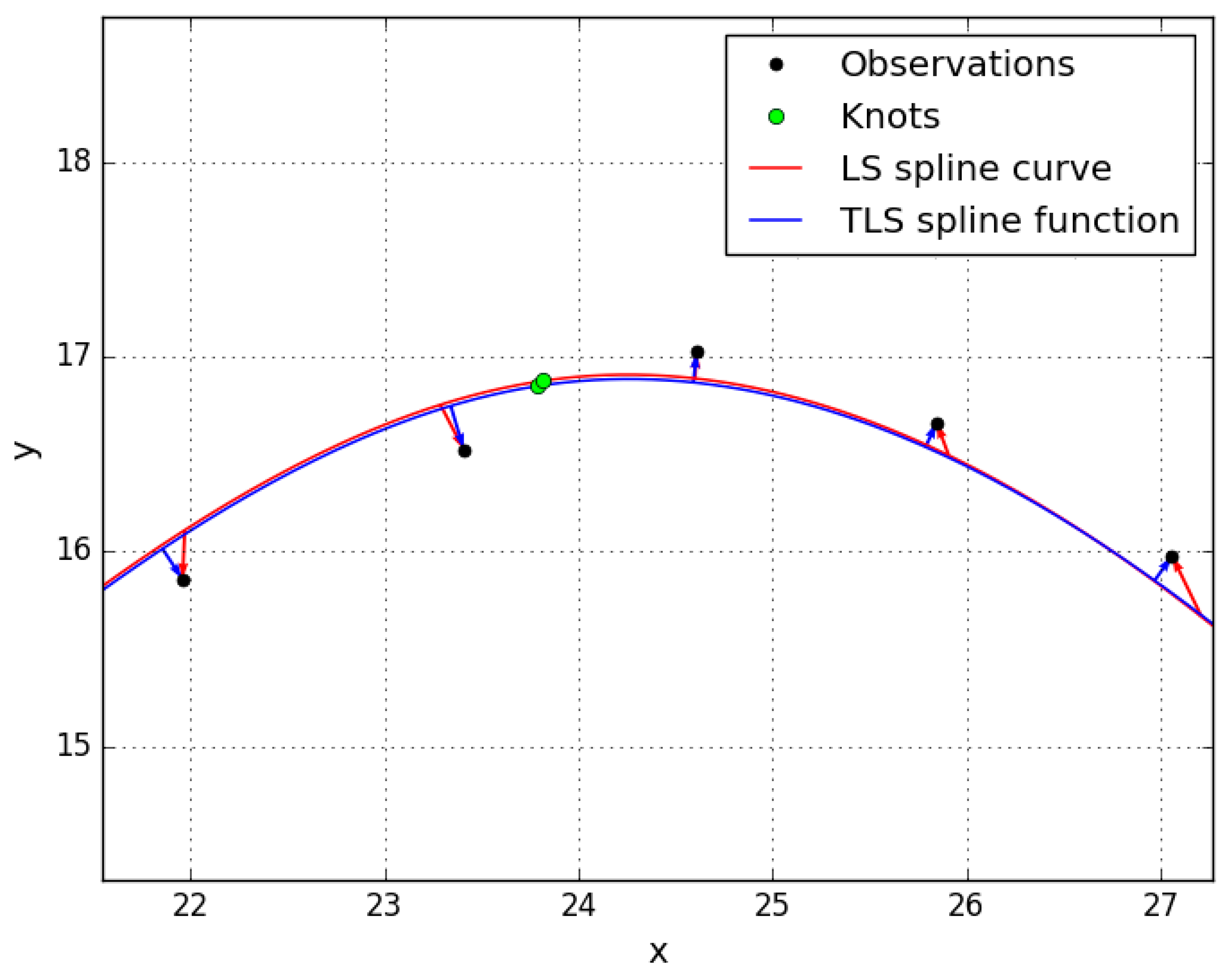
The results for Case 1 and Case 2.a are depicted in Figure 3, a magnification of the area marked by a rectangle is shown in Figure 4. The numerical values for the observation errors are listed in

Table 2. Error components from TLS and LS spline approximation.

Point	Case 1		Case 2.a		Case 2.b
	${\mathit{e}}_{{\mathit{x}}_{\mathbf{TLS}}}$	${\mathit{e}}_{{\mathit{y}}_{\mathbf{TLS}}}$	${\mathit{e}}_{{\mathit{x}}_{\mathbf{LS}}}$	${\mathit{e}}_{{\mathit{y}}_{\mathbf{LS}}}$	${\mathit{e}}_{{\mathit{x}}_{\mathbf{LS}}}$	${\mathit{e}}_{{\mathit{y}}_{\mathbf{LS}}}$
1	0.0286	−0.0217	0.0274	−0.0058	0.0118	0.1954
2	−0.0644	0.0684	−0.0715	0.0404	−0.0391	−0.2529
3	0.0292	−0.0488	0.0225	−0.0598	0.0258	−0.2995
4	0.0045	−0.0155	0.0606	0.0118	0.0097	−0.0128
5	0.0039	−0.0721	0.0060	−0.0604	0.0279	0.1192
6	0.0070	0.0553	−0.0491	0.0588	0.0163	0.3405
7	0.0376	0.1490	−0.0686	0.1566	−0.0031	0.4266
8	0.0037	0.0118	0.0641	−0.0283	−0.0793	0.1472
9	−0.0408	−0.1417	0.0337	−0.1719	−0.1223	−0.2025
10	−0.0063	−0.0324	−0.0282	−0.0188	−0.0400	−0.2721
11	−0.0009	−0.1615	0.0654	−0.1398	0.0670	−0.5328
12	−0.0246	0.1071	−0.0488	0.1233	0.1357	−0.2524
13	−0.1080	0.1914	−0.0557	0.2260	0.1543	0.0541
14	−0.0844	0.1068	0.0029	0.1640	0.0989	0.2499
15	−0.0300	0.0344	0.0068	0.0463	−0.0496	0.2926
16	0.1486	−0.1779	0.0211	−0.3057	−0.0869	0.0775
17	0.1035	−0.1568	−0.0111	−0.2528	−0.2471	0.1072
18	0.0669	−0.2246	0.1203	−0.2305	−0.1714	0.0386
19	0.0163	0.1570	0.0080	0.1364	−0.0662	0.2322
20	0.0556	0.1266	−0.0629	0.1692	0.1140	−0.0808
21	0.0899	0.1262	−0.1529	0.3136	0.2207	−0.2843
22	0.0838	0.0864	0.0095	0.1924	0.2008	−0.3201
23	−0.0398	−0.0349	0.0719	−0.1057	−0.0041	−0.1345
24	−0.0262	−0.0216	0.0987	−0.1050	−0.0486	0.2171
25	−0.1711	−0.1417	−0.0566	−0.2168	−0.1914	0.2269
26	−0.0501	−0.0446	0.0064	−0.0592	−0.0179	0.1687
27	−0.1120	−0.1188	−0.0143	−0.1769	−0.0468	−0.1908
28	0.0916	0.1241	−0.0505	0.2511	0.1224	−0.1052
29	0.0788	0.2075	0.0680	0.2211	0.1091	−0.0263
30	0.0023	−0.1372	−0.0228	−0.1737	−0.1005	0.0733

. With $x_i$, $y_i$, introduced as equally weighted and uncorrelated observations, the TLS solution yields error vectors that are orthogonal to the graph of the adjusted spline. In contrast, it is clearly visible in Figure 4 that the LS solution yields error vectors with “irregular” behavior, in the sense that they are far away from being orthogonal to the curve. Since the LS and the TLS solution refer to two different adjustment problems, the resulting adjusted graphs of the spline differ from each other. In this numerical example, the difference between the two adjusted graphs is rather small. The total sum of squared residuals (TSSR) for the TLS and for the LS solution are listed in

Table 3. Total sum of squared residuals (TSSR).

	Case 1	Case 2.a	Case 2.b
TSSR	0.578466	0.923518	1.968949

.

Figure 5 compares the result for Case 1 with the result for Case 2.b. In the magnification of the area marked by a rectangle shown in Figure 6 it is again clearly visible that the directions of the error vectors obtained from the LS solution are “irregular” and not orthogonal to the graph of the spline curve. Furthermore, if the length and direction of the error vectors for Case 2.a and Case 2.b are compared, a considerable influence of the chosen numerical values for the location parameter $t_i$ can be observed. In this numerical example the resulting adjusted graphs of the spline deviate considerably from each other. The corresponding TSSR values are listed in Table 3.

It can be concluded that both approaches have their advantages and disadvantages. Their application depends on the type of the phenomenon that is subject to the approximation. The parametric spline curve (LS solution) can be useful for geometrical approximation of arbitrary shapes where the interpretation of the errors is not the main focus since they vary with the choice of the values of the location parameter $t_i$. The error vectors obtained from the TLS approach can be utilized for deformation monitoring purposes, since they are orthogonal to the graph of the spline function in the case of equally weighted and uncorrelated observations.

It should be noted that the coordinates $x_i$ and $y_i$ captured with, e.g., a profile laser scanner are not original observations. They are based on the same angle and distance measurements and are, therefore, differently weighted and correlated. Since the precision of the distance measurement is influenced by a variety of factors, simplified assumptions about the stochastic model have often been used in the past. The intensity-based approach developed by Wujanz et al. [34] allows now to set up an appropriate stochastic model for 3D laser scanners. Based on this, Heinz et al. [35] have developed a stochastic model for a profile laser scanner. If a general stochastic model is used, the error vectors will no longer be strictly orthogonal to the adjusted spline, but it will be possible to apply statistical tests for outlier detection and deformation analysis.

7. Conclusions and Outlook

In this contribution, we have presented a total least squares spline approximation generated from a rigorous evaluation of an iteratively linearized Gauss-Helmert model under consideration of additional constraints for the unknowns. Similar to the approach for such problems proposed by Jazaeri et al. [9], the GH model allows introducing singular dispersion matrices for the observations.

Together with the basic methodology of spline approximation elaborated by Ezhov et al. [2], a clear und understandable formulation of spline approximation with both values $x_i$ and $y_i$ as observations is now available. This approach is of particular interest for engineering geodesy because the error vectors are orthogonal to the graph of the adjusted spline which has been demonstrated using a numerical example with equally weighted and uncorrelated observations. Hence, this approach is very suitable for the analysis of deformations.