Solving ODEs by Obtaining Purely Second Degree Multinomials via Branch and Bound with Admissible Heuristic †


Abstract
:1. Introduction
Structure of the Paper
2. Optimal Space Extension through Branch and Bound Optimization
2.1. Branch and Bound Optimization
2.2. Classical Quartic Anharmonic Oscillator as an Illustrative Example
2.3. Van Der Pol ODE as an Illustrative Example
2.4. Remarks on the Admissible Heuristic and Tie-Break
2.5. Implementation
2.6. Coping with Negative Integer Powers of Unknown Functions
Gravitational Two-Body Problem As an Illustrative Example
3. Probabilistic Evolution Theory Using the Condensed Kronecker Product
3.1. Brief Recall of Probabilistic Evolution Theory
3.2. Simplifying the Factorials
3.3. Cauchy Product Folding
3.4. Condensed Kronecker Product
3.4.1. The Two by Four Matrix as a Special Case
3.4.2. Generalization
- conKronProd (a, b) :=
- block ([i, j, c:[]],
- for i : 1 thru length (a) do
- (
- c : append (c, [a [i] ∗ b [i]]),
- for j : i + 1 thru length (a) do
- (
- c : append (c, [a [i] ∗ b [j]+b [i] ∗ a [j]])
- )
- ),
- return (c)
4. Conclusions
- The purpose of the paper is neither introducing probabilistic evolution theory, nor showing numerical implementations. That is done in certain previous works. Here, the focus is on space extension.
- Probabilistic evolution theory is not a simplified variant of B-series. The trees used in this work are for space extension; they are not for the expansion of the solution. Probabilistic evolution theory uses Kronecker power series for the solution. Combined with space extension, probabilistic evolution theory may be applied to a large set of problems. Probabilistic evolution theory has certain general aspects that make it applicable to both classical dynamical systems and quantum dynamical systems.
- For symbolic computation, we represent each multinomial right-hand side function as two lists of integers: one list for the terms (excluding the coefficients) and one list for the coefficients.
- By list manipulations, we find the optimal space extension by using branch and bound with an admissible heuristic.
- Up to now, space extension for obtaining purely second degree multinomials from multinomials (any degree) was intuitive: a manual trial and error effort. Although [18] was an important step in the formation of an algorithm, this paper gives the algorithm for performing space extension. The algorithm is based on branch and bound with an admissible heuristic.
- Branch and bound guarantees the minimum number of equations (optimal space extension), because it performs an exhaustive search.
- If there is more than one ODE set having the minimum number of equations, it is possible to obtain them one by one by using branch and bound search. It is enough to obtain one of the optimal (minimum number of equations) ODE sets for many applications.
- Branch and bound search is used in order to convert ODE with a multinomial (any degree) right-hand side to ODE with a purely second degree multinomial right-hand side. Therefore, the method is quite general.
- It is possible to use branch and bound search on ODEs having also negative integer powers of unknown functions in the right-hand sides. In this situation, we are a little more flexible in the search: we do not force optimality; we are interested in finding a very good space extension with small effort.
- When negative integer powers appear, the starting ODE set may become important. It is possible to use branch and bound for several obvious choices and to try to find the optimal space extension. Finding the ODE set to start the branch and bound is intuitive. This does not pose a problem: the gain acquired by choosing a better starting set is small.
- Branch and bound search may be improved by using a better heuristic. This is left for future works.
- Factorials appearing within the formulation of probabilistic evolution theory are simplified. Factorial behavior is embedded inside the recursion. This is a computational gain.
- The Cauchy product folding operation is defined. By using this operation, we are able to halve the number of terms to be summed to find a single . This is also an important computational gain.
- Cauchy product folding results in further simplifications because it puts a specific structure into the core matrix. It is possible to remove certain columns of this matrix and manipulate the vectors upon which the matrix acts. This does not change the numerical result. Instead of working with the matrix and n-element vectors, we can now work with the matrix and -element vectors. This is also an important computational gain.
- Calculation of these -element vectors is through the condensed Kronecker product: this is an operation proposed in this paper. It is a commutative operation. It takes two n-element vectors and forms a vector with elements. This operation is expected to be useful in areas other than probabilistic evolution theory, as well.
Author Contributions
Funding
Conflicts of Interest
References
- Hairer, E.; Wanner, G. Solving Ordinary Differential Equations II; Springer: Berlin/Heidelberg, Germany, 1996. [Google Scholar] [CrossRef]
- Butcher, J.C. Numerical Methods for Ordinary Differential Equations; Wiley Online Library: New York, NY, USA, 2008. [Google Scholar]
- Munthe-Kaas, H.Z.; Lundervold, A. On Post-Lie Algebras, Lie–Butcher Series and Moving Frames. Found. Comput. Math. 2013, 13, 583–613. [Google Scholar] [CrossRef] [Green Version]
- McLachlan, R.I.; Modin, K.; Munthe-Kaas, H.; Verdier, O. B-series methods are exactly the affine equivariant methods. Numer. Math. 2016, 133, 599–622. [Google Scholar] [CrossRef]
- Carothers, D.C.; Parker, G.E.; Sochacki, J.S.; Warne, P.G. Some properties of solutions to polynomial systems of differential equations. Electron. J. Differ. Equ. 2005, 2005, 1–17. [Google Scholar]
- Warne, P.; Warne, D.P.; Sochacki, J.; Parker, G.; Carothers, D. Explicit A-Priori error bounds and Adaptive error control for approximation of nonlinear initial value differential systems. Comput. Math. Appl. 2006, 52, 1695–1710. [Google Scholar] [CrossRef] [Green Version]
- Krattenthaler, C. Permutations with Restricted Patterns and Dyck Paths. Adv. Appl. Math. 2001, 27, 510–530. [Google Scholar] [CrossRef] [Green Version]
- Stanley, R.P. Enumerative Combinatorics. In Cambridge Studies in Advanced Mathematics; Cambridge University Press: Cambridge, UK, 1999; Volume 2. [Google Scholar]
- Gözükırmızı, C.; Kırkın, M.E.; Demiralp, M. Probabilistic evolution theory for the solution of explicit autonomous ordinary differential equations: Squarified telescope matrices. J. Math. Chem. 2017, 55, 175–194. [Google Scholar] [CrossRef]
- Demiralp, M. Probabilistic evolution theory in its basic aspects, and, its fundamental progressive stages. J. MESA 2018, 9, 245–275. [Google Scholar]
- Gözükırmızı, C.; Demiralp, M. Probabilistic evolution approach for the solution of explicit autonomous ordinary differential equations. Part 1: Arbitrariness and equipartition theorem in Kronecker power series. J. Math. Chem. 2014, 52, 866–880. [Google Scholar] [CrossRef]
- Gözükırmızı, C.; Demiralp, M. Probabilistic evolution approach for the solution of explicit autonomous ordinary differential equations. Part 2: Kernel separability, space extension, and, series solution via telescopic matrices. J. Math. Chem. 2014, 52, 881–898. [Google Scholar] [CrossRef]
- Gözükırmızı, C.; Demiralp, M. Constancy adding space extension for ODE sets with second degree multinomial right-hand side functions. AIP Conf. Proc. 2014, 1618, 875–878. [Google Scholar] [CrossRef]
- Demiralp, M. Squarificating the Telescope Matrix Images of Initial Value Vector in Probabilistic Evolution Theory (PET). In Proceedings of the 19th International Conference on Applied Mathematics (AMATH); WSEAS Press: Istanbul, Turkey, 2014; pp. 99–104. [Google Scholar]
- Gözükırmızı, C.; Tataroğlu, E. Squarification of telescope matrices in the probabilistic evolution theoretical approach to the two particle classical mechanics as an illustrative implementation. AIP Conf. Proc. 2017, 1798, 020062. [Google Scholar] [CrossRef]
- Gözükırmızı, C.; Kırkın, M.E. Classical symmetric fourth degree potential systems in probabilistic evolution theoretical perspective: Most facilitative conicalization and squarification of telescope matrices. AIP Conf. Proc. 2017, 1798, 020061. [Google Scholar] [CrossRef]
- Kırkın, M.E.; Demiralp, M. A Case Study on Squarification in Probabilistic Evolution Theory (PREVTH) for Henon-Heiles Systems. J. Comput. 2016, 1, 158–165. [Google Scholar]
- Gözükırmızı, C.; Demiralp, M. Probabilistic evolution theory for explicit autonomous ordinary differential equations: Recursion of squarified telescope matrices and optimal space extension. J. Math. Chem. 2018, 56, 1826–1848. [Google Scholar] [CrossRef]
- Demiralp, M. Promenading in the enchanted realm of Kronecker powers: Single monomial probabilistic evolution theory (PREVTH) in evolver dynamics. J. Math. Chem. 2018, 56, 2001–2023. [Google Scholar] [CrossRef]
- Demiralp, M.; Rabitz, H. Lie algebraic factorization of multivariable evolution operators: Definition and the solution of the canonical problem. Int. J. Eng. Sci. 1993, 31, 307–331. [Google Scholar] [CrossRef]
- Demiralp, M.; Rabitz, H. Lie algebraic factorization of multivariable evolution operators: Convergence theorems for the canonical case. Int. J. Eng. Sci. 1993, 31, 333–346. [Google Scholar] [CrossRef]
- Winston, P.H. Artificial Intelligence, 2nd ed.; Addison-Wesley Series in Computer Science; Addison-Wesley: Reading, PA, USA, 1984. [Google Scholar]
- Graham, R.; Lawler, E.; Lenstra, J.; Kan, A. Optimization and Approximation in Deterministic Sequencing and Scheduling: A Survey. In Discrete Optimization II; Hammer, P., Johnson, E., Korte, B., Eds.; Annals of Discrete Mathematics; Elsevier: Amsterdam, The Netherlands, 1979; Volume 5, pp. 287–326. [Google Scholar] [CrossRef]
- Lawler, E.L.; Wood, D.E. Branch-and-Bound Methods: A Survey. Oper. Res. 1966, 14, 699–719. [Google Scholar] [CrossRef]
- Kalay, B.; Demiralp, M. Somehow emancipating Probabilistic Evolution Theory (PREVTH) from singularities via getting single monomial PREVTH. J. Math. Chem. 2018, 56, 2024–2043. [Google Scholar] [CrossRef]
- Bayat Özdemir, S.; Demiralp, M. Using enchanted features of Constancy Adding Space Extension (CASE) to reduce the dimension of evolver dynamics: Single Monomial Probabilistic Evolution Theory. J. Math. Chem. 2018, 56, 2044–2068. [Google Scholar] [CrossRef]
- Eckstein, J.; Phillips, C.A.; Hart, W.E. Pico: An Object-Oriented Framework for Parallel Branch and Bound. In Inherently Parallel Algorithms in Feasibility and Optimization and their Applications; Butnariu, D., Censor, Y., Reich, S., Eds.; Studies in Computational Mathematics; Elsevier: Amsterdam, The Netherlands, 2001; Volume 8, pp. 219–265. [Google Scholar] [CrossRef]
- Gözükırmızı, C. Probabilistic evolution theory for explicit autonomous ODEs: Simplifying the factorials, Cauchy product folding and Kronecker product decomposition. AIP Conf. Proc. 2018, 2046, 020034. [Google Scholar] [CrossRef]


| Node Value | Score |
|---|---|
| 3+(0) | |
| 3+(1) | |
| 3+(1) | |
| 3+(2) | |
| 3+(1) | |
| 3+(2) | |
| 3+(0) | |
| 3+(1) | |
| 3+(1) | |
| 3+(2) | |
| 3+(1) | |
| 3+(2) |
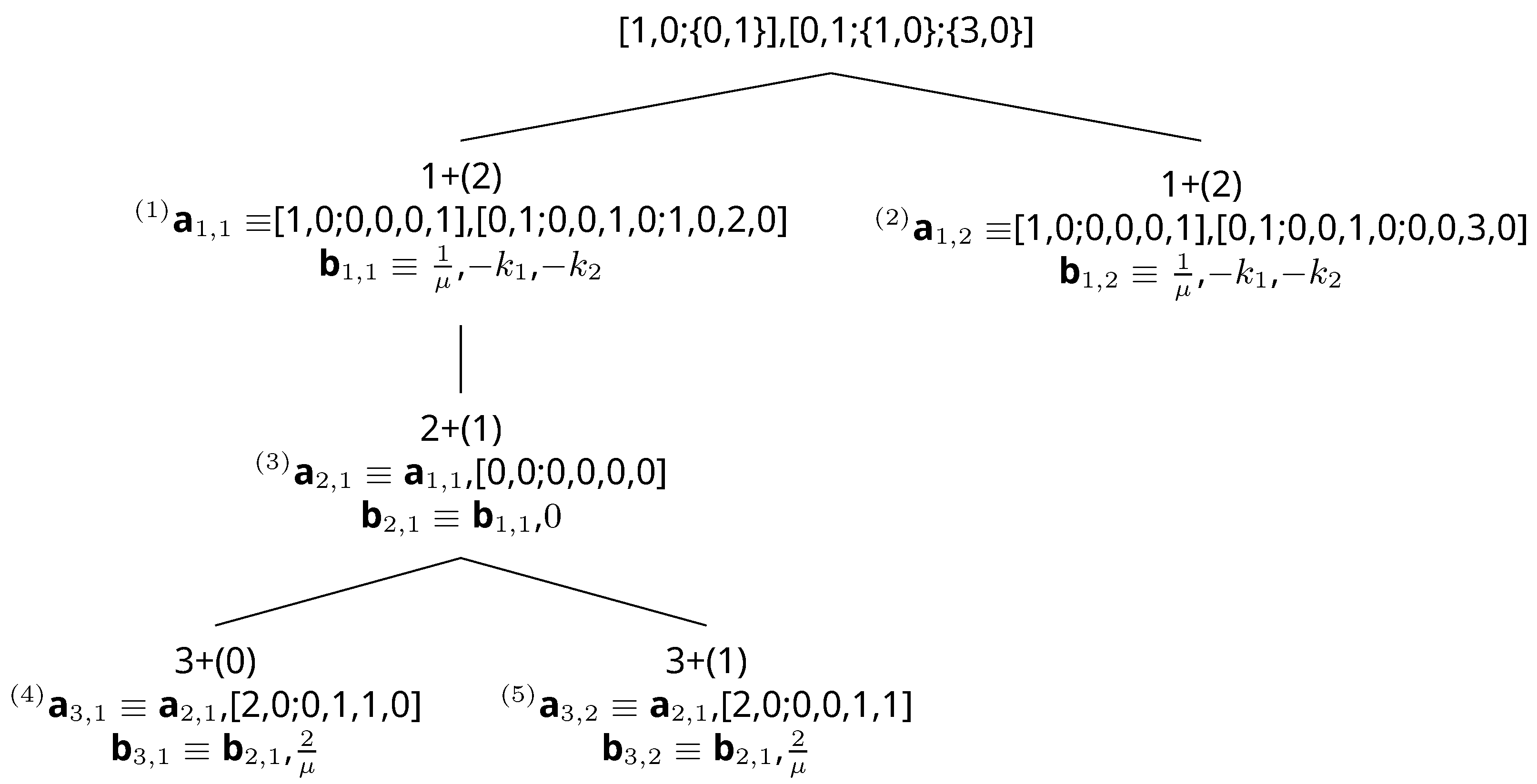
| Step | Explanation | Queue |
|---|---|---|
| 1 | One-element queue that contains the root node | [1,0;{0,1}], [0,1;{1,0};{3,0}] |
| 2 | The first path in the queue is dequeued and extended. The new paths are put into the queue, and the entire queue is sorted by score with smaller paths in front (right). When sorting by score, there is a tie. Paths are then sorted using reverse numerical order where the smaller path is in front. | [1,0;0,0,0,1], [0,1;0,0,1,0;0,0,3,0]; [1,0;0,0,0,1], [0,1;0,0,1,0;1,0,2,0] |
| 3 | The first path does not terminate at the goal. The first path in the queue is dequeued and extended. A new path is put into the queue, and the entire queue is sorted by score. Again, there is a tie; therefore, reverse numerical order is used. | [1,0;0,0,0,1], [0,1;0,0,1,0;0,0,3,0]; [1,0;0,0,0,1], [0,1;0,0,1,0;1,0,2,0], [0,0;0,0,0,0] |
| 4 | The first path in the queue does not terminate at the goal. The first path in the queue is dequeued and extended. New paths are put into the queue, and the entire queue is sorted by score with a smaller score in front. The first two paths have the same score. The first two paths are put in reverse numerical order where the smaller path is in front. | [1,0;0,0,0,1], [0,1;0,0,1,0;1,0,2,0], [0,0;0,0,0,0], [2,0;0,0,1,1]; [1,0;0,0,0,1], [0,1;0,0,1,0;0,0,3,0]; [1,0;0,0,0,1], [0,1;0,0,1,0;1,0,2,0], [0,0;0,0,0,0], [2,0;0,1,1,0] |
| 5 | The first path in the queue terminates at the goal. The first path in the queue is the optimal path. |
© 2019 by the authors. Licensee MDPI, Basel, Switzerland. This article is an open access article distributed under the terms and conditions of the Creative Commons Attribution (CC BY) license (http://creativecommons.org/licenses/by/4.0/).
Share and Cite
Gözükırmızı, C.; Demiralp, M. Solving ODEs by Obtaining Purely Second Degree Multinomials via Branch and Bound with Admissible Heuristic. Mathematics 2019, 7, 367. https://doi.org/10.3390/math7040367
Gözükırmızı C, Demiralp M. Solving ODEs by Obtaining Purely Second Degree Multinomials via Branch and Bound with Admissible Heuristic. Mathematics. 2019; 7(4):367. https://doi.org/10.3390/math7040367
Chicago/Turabian StyleGözükırmızı, Coşar, and Metin Demiralp. 2019. "Solving ODEs by Obtaining Purely Second Degree Multinomials via Branch and Bound with Admissible Heuristic" Mathematics 7, no. 4: 367. https://doi.org/10.3390/math7040367