Article

Global Stability Analysis of Two-Stage Quarantine-Isolation Model with Holling Type II Incidence Function

Department of Mathematics, Hashemite University, P.O. Box 330127, Zarqa 13133, Jordan
Mathematics 2019, 7(4), 350; https://doi.org/10.3390/math7040350
Submission received: 28 February 2019 / Revised: 27 March 2019 / Accepted: 10 April 2019 / Published: 15 April 2019
(This article belongs to the Section Mathematics and Computer Science)

Abstract

:
A new two-stage model for assessing the effect of basic control measures, quarantine and isolation, on a general disease transmission dynamic in a population is designed and rigorously analyzed. The model uses the Holling II incidence function for the infection rate. First, the basic reproduction number ( R 0 ) is determined. The model has both locally and globally asymptotically stable disease-free equilibrium whenever R 0 < 1 . If R 0 > 1 , then the disease is shown to be uniformly persistent. The model has a unique endemic equilibrium when R 0 > 1 . A nonlinear Lyapunov function is used in conjunction with LaSalle Invariance Principle to show that the endemic equilibrium is globally asymptotically stable for a special case.

1. Introduction

Over the decades, quarantine (of individuals suspected of being exposed to a communicable disease) and isolation (of individuals with disease symptoms) have been widely used to control the spread of numerous communicable diseases, such as pandemic influenza, cholera, Ebola, Severe Acute Respiratory Syndrome (SARS), and most recently swine influenza pandemic [1,2,3,4,5,6,7,8,9]. Numerous mathematical models have been studying the effect of quarantine and isolation in combatting the spread of the diseases (see, for instance, refs. [1,2,4,5,6,7,8,10,11,12,13] and the references therein). In the aforementioned studies, mass action or standard incidence functions were used in the modeling of the transmission dynamics of the diseases. In this study, another nonlinear incidence function (called the Holling type II incidence function) will be used in the modeling of the transmission dynamics of a general disease. The Holling type II incidence function is given by g ( I ) = β I 1 + α I , with α > 0 , where I is the number of infectious individuals and β is the effective contact rate (the average number of contacts sufficient for transmitting infection). The incidence function g ( I ) was first used in the study of the cholera epidemic in Bari, Italy by Capasso and Serio [14]. The reason for using the Holling type II incidence functional comes from the information that the number of effective contacts between susceptible individuals and infective individuals may saturate at very high levels due to behavioral changes or due to crowding of infective people taken by the people in reaction to the severity of the disease [15,16]. It is well known that some infectious diseases, such as influenza [17] and HIV [18], have multiple disease (infection) stages in their transmission dynamics.
The main purpose of this study is to offer a deep qualitative analysis of a new two-stage model for the transmission dynamics of a disease that can be controlled by using quarantine and isolation, where the Holling type II incidence function is used.
The paper is organized as follows. The formulation of the model is given in Section 2. The local and global asymptotic stability of the disease-free equilibrium (DFE) is analyzed in Section 3. The existence of the endemic equilibrium is provided in Section 4. Global stability proof for the endemic equilibrium for the special case is also analyzed using a nonlinear Lyapunov function.

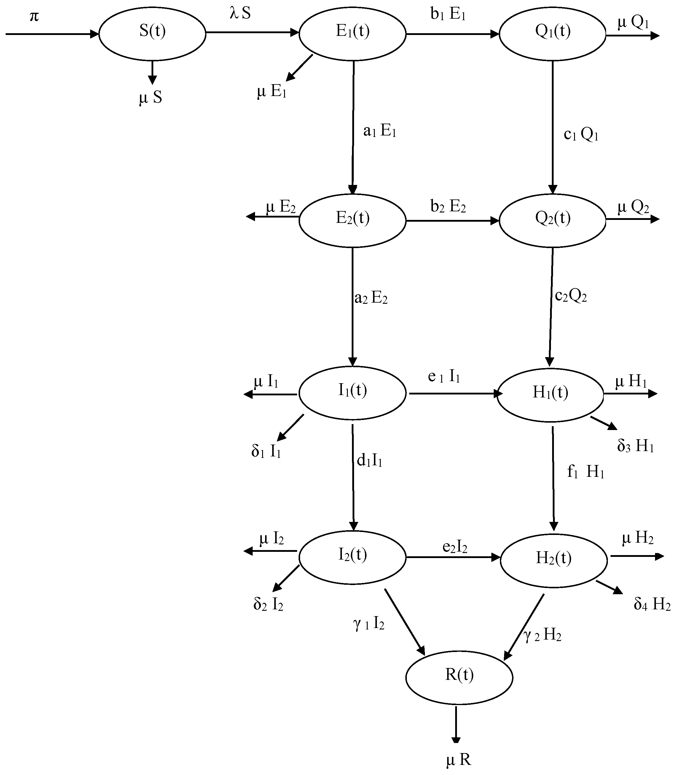
2. Model Formulation

The total population at time t, denoted by N ( t ) is sub-divided into ten compartments of susceptible ( S ( t ) ) , exposed (with two stages ( E 1 ( t ) E 2 ( t ) ), infectious individuals (with two stages ( I 1 ( t ) I 2 ( t ) ), Isolated individuals (with two stages H 1 ( t ) H 2 ( t ) ), and recovered ( R ( t ) ) individuals, so that
N ( t ) = S ( t ) + E 1 ( t ) + E 2 ( t ) + Q 1 ( t ) + Q 2 ( t ) + I 1 ( t ) + I 2 ( t ) + H 1 ( t ) + H 2 ( t ) + R ( t ) .
The model is given by the following system of nonlinear differential equations
d S d t = Π ( λ ( t ) + μ ) S ( t ) , d E 1 d t = λ ( t ) S ( t ) ( a 1 + b 1 + μ ) E 1 ( t ) , d E 2 d t = a 1 E 1 ( a 2 + b 2 + μ ) E 2 ( t ) , d Q 1 d t = b 1 E 1 ( c 1 + μ ) Q 1 , d Q 2 d t = c 1 Q 1 + b 2 E 2 ( c 2 + μ ) Q 2 , d I 1 d t = a 2 E 2 ( t ) ( d 1 + e 1 + δ 1 + μ ) I 1 ( t ) , d I 2 d t = d 1 I 1 ( t ) ( e 2 + γ 1 + δ 2 + μ ) I 2 ( t ) , d H 1 d t = c 2 Q 2 + e 1 I 1 ( f 1 + δ 3 + μ ) H 1 , d H 2 d t = f 1 H 1 + e 2 I 2 ( γ 2 + δ 4 + μ ) H 2 , d R d l t = γ 1 I 2 ( t ) + γ 2 H 2 ( t ) μ R ( t ) ,
where λ ( t ) is the infection rate given by
λ ( t ) = β I 1 1 + α 1 I 1 + η I 2 1 + α 2 I 2 .
In (2), β represents the effective contact rate, where 0 < η < 1 is a parameter that accounts for the reduction in disease transmission given by infectious individuals ( I 1 ) in comparison to infectious individuals in the I 2 stage.
Susceptible people ( S ) is increased by the recruitment of individuals into the population, at a rate Π . This class is decreased by infection (with the rate of λ ). Furthermore, this population is decreased by natural death (at a rate μ ; populations in all classes are assumed to have the same natural death rate).
Exposed individuals in stage 1 ( E 1 ) are generated with the rate of λ and reduced by progression to the next exposed stage ( E 2 ; at a rate a 1 ) and quarantine (at a rate b 1 ). Exposed individuals in stage 2 are generated at the rate a 1 . This population is decreased by the development of clinical symptoms of the disease (at a rate a 2 ) and quarantine (at a rate b 2 ).
The class of quarantined individuals in stage 1 is increased by quarantine of exposed people in stage E 1 (at the rate b 1 ) and it is reduced by progression to the second quarantined stage (at a rate c 1 ). Similarly, quarantined people in stage 2 are increased by the quarantine of exposed people in the second stage (at the rate b 2 ) and the progression of quarantined people from the first stage into the second stage (at the rate c 1 ). It is decreased by hospitalization (at a rate c 2 ).
The infectious people in stage 1 are increased when exposed people in the second stage develop symptoms (at the rate a 2 ). It is reduced by progression to the second infectious stage (at a rate d 1 ), hospitalization (isolation) (at a rate e 1 ) and disease-induced death (at a rate δ 1 ). The population of infectious class in the second stage is generated by progression of individuals in the first stage (at a rate d 1 ). It is reduced by isolation (at a rate e 2 ), recovery (at a rate γ 1 ) and disease-induced death (at a rate δ 2 ).
The population of Isolated individuals in the first stage is increased by the hospitalization of infectious people in stage 1 (at the rate e 1 ) and quarantined individuals in the second stage (at the rate c 2 ). It is decreased by progression to the second Isolated stage (at a rate f 1 ), and disease-induced death (at a rate δ 3 ). The population of Isolated individuals in the second stage is generated by the progression of Isolated individuals from the first stage into the second one (at the rate f 1 ). It is decreased by recovery (a rate γ 2 ) and disease-induced death (at a rate δ 4 ).
Finally, the recovered individuals is increased by the recovery of infectious individuals and hospitalization individuals (at the rates γ 1 and γ 2 , respectively). It is reduced by natural death (at the rate μ ). (A flow diagram of the model is depicted in Figure 1. The associated variables and parameters are described in Table 1):
It should be noted the model (1) is different by the basic model considered in [19] by
(a)
Using a Holling type incidence function to model the infection rate (the standard incidence function was used in [19])
(b)
Considering two stages for the infectious compartments (Exposed, infected, quarantined, and isolated compartments)

2.1. Preliminaries and Basic Properties

Since the model (1) for human populations, all its parameters are non-negative. Furthermore, the following non-negativity result holds.
Theorem 1.
All variables of the model (1) are non-negative for all t > 0 . This mean, the solutions of system (1) with positive initial conditions will remain positive for all time t > 0 .
Proof. 
Let
t 1 = sup { t > 0 : S > 0 , E 1 > 0 , E 2 > 0 , Q 1 > 0 , Q 2 > 0 , I 1 > 0 , I 2 > 0 , H 1 > 0 , H 2 > 0 , R > 0 [ 0 , t ] } .
Hence, t 1 > 0 . From the first equation of the system (1) it follows that
d d t S ( t ) exp μ t + 0 t λ ( τ ) d τ = Π exp μ t + 0 t λ ( τ ) d τ .
which gives,
S ( t 1 ) exp μ t 1 + 0 t 1 λ ( τ ) d τ S ( 0 ) = 0 t 1 Π exp μ y + 0 y λ ( τ ) d τ d y ,
hence,
S ( t ) = S ( 0 ) exp μ t 1 0 t 1 λ ( τ ) d τ exp μ t 1 0 t 1 λ ( τ ) d τ 0 t 1 Π exp μ y + 0 y λ ( τ ) d τ d y > 0 .
In the same way, it can be shown that E 1 > 0 , E 2 > 0 , Q 1 > 0 , Q 2 > 0 , I 1 > 0 , I 2 > 0 , H 1 > 0 , H 2 > 0 and R > 0 for all time t > 0 . □
Lemma 1.
The closed set
D = ( S , E 1 , E 2 , Q 1 , Q 2 , I 1 , I 2 , H 1 , H 2 , R ) R + 10 : S + E 1 + E 2 + Q 1 + Q 2 + I 1 + I 2 + H 1 + H 2 + R Π μ
is positively invariant.
Proof. 
Adding all the equations of the model (1) gives,
d N d t = Π μ N ( δ 1 I 1 + δ 2 I 2 + δ 3 H 1 + δ 4 H 2 ) .
It follows that d N d t Π μ N , thus d N d t 0 provided that N Π μ . By using standard comparison theorem [20] it can be shown that N N ( 0 ) e μ t + Π μ ( 1 e μ t ) . In particular, N ( t ) Π μ if N ( 0 ) Π μ . Thus, the region D is positively invariant. Furthermore, if N ( 0 ) > Π μ , then either the solution enters D in finite time, or N ( t ) approaches Π μ asymptotically. Hence, the region D attracts all solutions in R + 10 . □
Since the region D is positively invariant, it is sufficient to consider the dynamics of the flow generated by the model (1) in D , where the usual existence, uniqueness, continuation results hold for the system [21].

Next-Generation Method

Suppose that the population is divided into n compartments, with m < n infected compartments. At time t , let x i ( t ) be the number of infected individuals in the i t h infected class such that
d x i d t = F i ( x ) V i ( x ) , with V i = V i ( x ) V i + ( x ) for i = 1 , 2 , , m ,
where F i ( x ) represents the rate of appearance of new infections in class i, V i + ( x ) represents the rate of transfer of individuals into class i by all other means, and V i ( x ) represents the rate of transfer of individuals out of class i. System can be rewritten as follows
X ˙ = F ( X ) V ( X ) ,
with, F ( X ) = ( F 1 , F 2 , , F m ) T and V ( X ) = ( V 1 , V 2 , , V m ) T .
Lemma 2.
(van den Driessche and Watmough [22]). If x ¯ is a DFE of (5), then the derivatives D F ( x ¯ ) and D V ( x ¯ ) are partitioned as
D F ( x ¯ ) = F 0 0 0 ,   D V ( x ¯ ) = V 0 J 3 J 4 ,
where F and V are the m × m matrices defined by,
F = F i x j ( x ¯ )   a n d   V = V i x j ( x ¯ )   w i t h   1 i ,   j m .
Furthermore, F is non-negative, V is a non-singular M matrix and J 3 , J 4 are matrices associated with the transition terms of the model, and all eigenvalues of J 4 have positive real parts.
Now, the next-generation matrix is given by F V 1 and the spectral radius (the largest eigenvalue) of F V 1 is the basic reproduction number of the model (5) [22].

3. Stability of DFE

3.1. Local Stability

The DFE of the model (1) is given by
E 0 = ( S * , E 1 * , E 2 * , Q 1 * , Q 2 * , I 1 * , I 2 * , H 1 * , H 2 * , R * ) = ( Π / μ , 0 , 0 , 0 , 0 , 0 , 0 , 0 , 0 , 0 ) .
The next-generation operator method [22,23] will be used to analyze the stability of E 0 . Using the same notation in the previous section, the non-negative matrix, F and the M-matrix, V are given by
F = 0 0 0 0 β Π μ η β Π μ 0 0 0 0 0 0 0 0 0 0 0 0 0 0 0 0 0 0 0 0 0 0 0 0 0 0 0 0 0 0 0 0 0 0 0 0 0 0 0 0 0 0 0 0 0 0 0 0 0 0 0 0 0 0 0 0 0 0 ,
and,
V = k 1 0 0 0 0 0 0 0 a 1 k 2 0 0 0 0 0 0 b 1 0 k 3 0 0 0 0 0 0 b 2 c 1 k 4 0 0 0 0 0 a 2 0 0 k 5 0 0 0 0 0 0 0 d 1 k 6 0 0 0 0 0 c 2 e 1 0 k 7 0 0 0 0 0 0 e 2 f 1 k 8 .
The control reproduction number [24,25], denoted by R 0 = ρ ( F V 1 ) is given by
R 0 = β Π a 1 a 2 ( k 6 + η d 1 ) μ k 1 k 2 k 5 k 6 ,
where,
k 1 = μ + a 1 + b 1 , k 2 = μ + a 2 + b 2 , k 3 = μ + c 1 , k 4 = μ + c 2 , k 5 = μ + δ 1 + d 1 + e 1 , k 6 = μ + δ 2 + γ 1 + e 2 , k 7 = μ + δ 3 + f 1 , k 8 = μ + δ 4 + γ 2 .
The following result is established by using Theorem 2 in [22].
Lemma 3.
The model (1) has a locally asymptotically stable (LAS) DFE whenever R 0 < 1 . Moreover, the DFE of this model is unstable if R 0 > 1 .
The average number of new infections generated by a single infectious individual in a population is measured by the quantity R 0 . The epidemiological implication of Lemma 3 is that the disease dies out from the population (when R 0 < 1 ) if the initial sizes of the sub-populations of the model are in the basin of attraction of the DFE ( E 0 ). To make sure that disease dies out form the population regardless of the initial sizes of sub-populations, it is necessary to show that the DFE is globally asymptotically stable (GAS) if R 0 < 1 . This is established below.

3.2. Global Stability of DFE

Theorem 2.
The model (1) has GAS DFE, given by (6), in D whenever R 0 1 .
Proof. 
Define the following Lyapunov function:
F = a 1 a 2 ( k 6 + η d 1 ) η k 1 k 2 k 5 E 1 + a 1 ( k 6 + η d 1 ) η k 2 k 5 E 2 + k 6 + η d 1 η k 5 I 1 + I 2 ,
differentiate F with respect to t gives
F ˙ = a 1 a 2 ( k 6 + η d 1 ) η k 1 k 2 k 5 E ˙ 1 + a 2 ( k 6 + η d 1 ) η k 2 k 5 E ˙ 2 + k 6 + η d 1 η k 5 I ˙ 1 + I ˙ 2 = a 1 a 2 ( k 6 + η d 1 ) η k 1 k 2 k 5 β S I 1 1 + α 1 I 1 + η I 2 1 + α 2 I 2 k 1 E 1 + a 2 ( k 6 + η d 1 ) η k 2 k 5 a 1 E 1 k 2 E 2 + k 6 + η d 1 η k 5 a 2 E 2 k 5 I 1 + d 1 I 1 k 6 I 2 a 1 a 2 ( k 6 + η d 1 ) η k 1 k 2 k 5 β Π μ ( I 1 + η I 2 ) k 1 E 1 + a 2 ( k 6 + η d 1 ) η k 2 k 5 a 1 E 1 k 2 E 2 + k 6 + η d 1 η k 5 a 2 E 2 k 5 I 1 + d 1 I 1 k 6 I 2 = β Π a 1 a 2 ( k 6 + η d 1 ) μ η k 1 k 2 k 5 ( I 1 + η I 2 ) + d 1 k 6 + η d 1 η I 1 k 6 I 2 = k 6 η ( R 0 1 ) ( I 1 + η I 2 )
Since all the variables and the parameters of the model (1) are non-negative, it follows that F ˙ 0 for R 0 1 with F ˙ = 0 if and only if E = I u = I e = 0 . Thus, F defined a Lyapunov function on D . Hence,
( E 1 , E 2 , I 1 , I 2 ) ( 0 , 0 , 0 , 0 ) as t .
It can be easily shown that ( Q 1 , Q 2 , H 1 , H 2 , R ) ( 0 , 0 , 0 , 0 , 0 ) and S Π μ as t . Furthermore, the region D is an invariant and attracting set of R + 10 , and the largest compact invariant set in ( S , E 1 , E 2 , Q 1 , Q 2 , I 1 , I 2 , H 1 , H 2 , R ) D : F = 0 is the singleton { E 0 } . Thus, by Invariance Principle [26], every solution of the system (1), and initial conditions in R + 10 , approaches the DFE ( E 0 ) as t whenever R 0 < 1 . □
The above result shows that the disease dies out from the population if the reproduction number of the model is less than one. The epidemiological implication of the above theorem is that the use of isolation and quarantine can lead to elimination of the disease if both controls can keep the threshold quantity, R 0 , to a value less than unity (i.e., The condition R 0 < 1 is sufficient and necessary for the elimination of the disease ). Figure 2 illustrate numerical results obtained by simulating the model (1) using various initial conditions for the case R 0 < 1 . Its clear that the solutions are converged to the DFE.

4. Existence and Stability for Endemic Equilibrium Point

4.1. Persistence of the Disease

The persistence of the disease in the population will be investigated below. The model system (1) is said to be uniformly persistent if there exists a constant c such that any solution ( S ( t ) , E 1 ( t ) , E 2 ( t ) , Q 1 ( t ) , Q 2 ( t ) , I 1 ( t ) , I 2 ( t ) , H 1 ( t ) , H 2 ( t ) , R ( t ) ) satisfies ([27,28]):
lim inf t S ( t ) c , lim inf t E 1 ( t ) c , lim inf t E 2 ( t ) c , lim inf t Q 1 ( t ) c , lim inf t Q 2 ( t ) c , lim inf t I 1 ( t ) c , lim inf t I 2 ( t ) c , lim inf t H 1 ( t ) c , lim inf t H 2 ( t ) c , lim inf t R ( t ) c ,
provided that ( S ( 0 ) , E 1 ( 0 ) , E 2 ( 0 ) , Q 1 ( 0 ) , Q 2 ( 0 ) , I 1 ( 0 ) , I 2 ( 0 ) , H 1 ( 0 ) , H 2 ( 0 ) , R ( 0 ) ) D .
Theorem 3.
The model (1) is uniformly persistent in D if and only if R 0 > 1 .
Proof. 
The proof of the above theorem follows from using the same approach given in [29] to prove Proposition 3.3 of [29], which is applying a uniform persistence theorem in [27] and noting that the DFE of the model (1) is unstable whenever R 0 > 1 (Lemma 3). □
Whenever R 0 > 1 its clear (from Theorem (3)) that the model (1) is uniformly persistent. Moreover using Theorem 2.8.6 in [30] and Theorem D.3 in [20] gives the model (1) has at least one endemic equilibrium in D . Hence, the following Lemma is concluded.
Lemma 4.
System (1) has at least one endemic equilibrium provided that R 0 > 1 .
The uniqueness of this equilibrium will be analyzed in the coming subsection.

4.2. Uniqueness of Endemic Equilibrium Point (EEP)

Let,
E 1 = ( S * * , E 1 * * , E 2 * * , Q 1 * * , Q 2 * * , I 1 * * , I 2 * * , H 1 * * , H 2 * * , R * * )
represents any arbitrary EEP of the model (1). Furthermore, define
λ * * = β I 1 * * 1 + α 1 I 1 * * + β η I 2 * * 1 + α 2 I 2 * *
(the force of infection of the model (1) at steady-state). It follows, by solving the equations in (1) at steady-state that
S * * = Π λ * * + μ , E 1 * * = Π λ * * ( λ * * + μ ) k 1 , E 2 * * = a 1 Π λ * * ( λ * * + μ ) k 1 k 2 , Q 1 * * = b 1 Π λ * * ( λ * * + μ ) k 1 k 3 , Q 2 * * = ( a 1 b 2 k 3 + b 1 c 1 k 2 ) Π λ * * ( λ * * + μ ) k 1 k 2 k 3 k 4 , I 1 * * = a 1 a 2 Π λ * * ( λ * * + μ ) k 1 k 2 k 5 , I 2 * * = a 1 a 2 d 1 Π λ * * ( λ * * + μ ) k 1 k 2 k 5 k 6 .
Substituting I 1 * * and I 2 * * in (9) into (8) gives the following quadratic equation (in terms of λ * * ):
M 0 ( λ * * ) 2 + M 1 λ * * + M 2 = 0 ,
with,
M 0 = ( Π a 1 a 2 α 1 + k 1 k 2 k 5 ) ( Π a 1 a 2 d 1 α 2 + k 1 k 2 k 5 k 6 ) , M 1 = Π 2 a 1 2 a 2 2 α 1 d 1 η β Π 2 a 1 2 a 2 2 α 2 d 1 β Π a 1 a 2 k 1 k 2 k 5 k 6 β Π a 1 a 2 d 1 k 1 k 2 k 5 η β + Π a 1 a 2 k 1 k 2 k 5 k 6 α 1 μ + Π a 1 a 2 d 1 k 1 k 2 k 5 α 2 μ + 2 μ k 1 2 k 2 2 k 5 2 k 6 , M 2 = μ 2 k 1 2 k 2 2 k 5 2 k 6 ( 1 R 0 ) .
By solving for λ * * in (10) and substituting the positive values of λ * * into the expressions in (9) the endemic equilibria of the model (1) can then be obtained. It should be noted that M 0 > 0 and M 2 < 0 whenever R 0 > 1 . Thus, by using the Descartes Rule of Signs on the quadratic Equation (10), the following result is established.
Lemma 5.
The model (1) has a unique endemic (positive) equilibrium, given by E 1 whenever R 0 > 1 .

4.3. Global Stability for Endemic Equilibrium

In this section, the global stability of the endemic equilibrium of the model (1) is given for the special case where the associated disease-induced mortality in all classes is negligible (so that δ 1 = δ 2 = δ 3 = δ 4 = 0 ).
Define
R s = R 0 | δ 1 = δ 2 = δ 3 = δ 4 = 0
D 0 = ( S , E 1 , E 2 , Q 1 , Q 2 , I 1 , I 2 , H 1 , H 2 , R ) D : E 1 = E 2 = I 1 = I 2 = H 1 = H 2 = R = 0 .
We claim the following result,
Theorem 4.
The endemic equilibrium of the model (1) with δ 1 = δ 2 = δ 3 = δ 4 = 0 is GAS in D \ D 0 if R s > 1 .
Proof. 
Let R s > 1 , such that the endemic equilibrium exists. Furthermore, define the following Lyapunov function:
F = 1 2 ( S S * * ) + ( E 1 E 1 * * ) + ( E 1 E 1 * * ) + ( Q 1 Q 1 * * ) + ( Q 2 Q 2 * * ) + ( I 1 I 1 * * ) + ( I 2 I 2 * * ) + ( H 1 H 1 * * ) + ( H 2 H 2 * * ) + ( R R * * ) 2
with Lyapunov derivative
F ˙ = ( S S * * ) + ( E 1 E 1 * * ) + ( E 2 E 2 * * ) + ( Q 1 Q 1 * * ) + ( Q 2 Q 2 * * ) + ( I 1 I 1 * * ) + ( I 2 I 2 * * ) + ( H 1 H 1 * * ) + ( H 2 H 2 * * ) + ( R R * * ) N ˙ ( t ) .
Since S * * + E 1 * * + E 2 * * + Q 1 * * + Q 2 * * + I 1 * * + I 2 * * + H 1 * * + H 2 * * + R * * = Π μ and N ˙ ( t ) = Π μ N ( t ) it follows that
F ˙ = N ( t ) Π μ Π μ N ( t ) = 1 μ μ N ( t ) Π Π μ N ( t ) = 1 μ Π μ N ( t ) 2 .
It follows that F ˙ 0 for R s > 1 with F ˙ = 0 if and only if S = S * * , E 1 = E 1 * * , E 2 = E 2 * * , Q 1 = Q 1 * * , Q 2 = Q 2 * * , I 1 = I 1 * * , I 2 = I 2 * * , H 1 = H 1 * * , H 2 = H 2 * * , and R = R * * . Hence, F is a Lyapunov function on D \ D 0 . Thus, S ( t ) S * * , E 1 ( t ) E 1 * * , E 2 ( t ) E 2 * * , Q 1 ( t ) Q 1 * * , Q 2 ( t ) Q 2 * * , I 1 ( t ) I 1 * * , I 2 ( t ) I 2 * * , H 1 ( t ) H 1 * * , H 2 ( t ) H 2 * * , and R ( t ) R * * as t . The proof is concluded as in the proof of Theorem 2. Thus, the unique endemic equilibrium of the model (1) with δ 1 = δ 2 = δ 3 = δ 4 = 0 is GAS in D \ D 0 whenever R s > 1 . The epidemiological implication of the above result is that the disease will persist in the community (with the use of isolation and quarantine) if threshold quantity ( R s ) exceeds unity. Numerical simulation results, done in Figure 3 show convergence to the EEP for the case when R 0 > 1 .

5. Conclusions

In this paper, a new two stages quarantine/isolation model with a nonlinear incidence rate is designed and rigorously analyzed. The model, which consists of ten mutually exclusive epidemiological compartments, uses the Holling type II incidence function for the infection rate. Some of the theoretical findings of the study are the following:
(i)
The model (1) has a locally asymptotically stable DFE if the associated reproduction number ( R 0 ) is less than one.
(ii)
The model (1) has a GAS whenever R 0 < 1 .
(iii)
System (1) is uniformly persistent in D if and only if the reproduction number exceeds unity.
(iv)
The model has a unique endemic equilibrium whenever R 0 > 1 .
(v)
The unique endemic equilibrium of the model is shown to be GAS for a special case.

Funding

This research received no external funding.

Acknowledgments

The author is grateful to the anonymous reviewers for their constructive comments.

Conflicts of Interest

The author declares no conflict of interest.

References

  1. Chowell, G.; Hengartner, N.W.; Castillo-Chavez, C.; Fenimore, P.W.; Hyman, J.M. The basic reproductive number of ebola and the effects of public health measures: The cases of Congo and Uganda. J. Theor. Biol. 2004, 1, 119–126. [Google Scholar] [CrossRef] [PubMed]
  2. Donnelly, C.; Ghani, A.; Leung, G.; Hedley, A.; Fraser, C.; Riley, S.; Abu-Raddad, L.J.; Ho, L.M.; Thach, T.Q.; Chau, P.; et al. Epidemiological determinants of spread of casual agnet of severe acute respiratory syndrome in Hong Kong. Lancet 2003, 361, 1761–1766. [Google Scholar] [CrossRef]
  3. Hethcote, H.W.; Zhien, M.; Shengbing, L. Effects of quarantine in six endemic models for infectious diseases. Math. Biosci. 2002, 180, 141–160. [Google Scholar] [CrossRef]
  4. Lipsitch, M.; Cohen, T.; Cooper, B.; Robins, J.M.; Ma, S.; James, L.; Gopalakrishna, G.; Chew, S.K.; Tan, C.C.; Samore, M.H.; et al. Transmission dynamics and control of severe acute respiratory syndrome. Science 2003, 300, 1966–1970. [Google Scholar] [CrossRef] [PubMed]
  5. Lloyd-Smith, J.O.; Galvani, A.P.; Getz, W.M. Curtailing transmission of severe acute respiratory syndrome within a community and its hospital. Proc. R. Soc. Lond. B 2003, 170, 1979–1989. [Google Scholar] [CrossRef] [PubMed]
  6. McLeod, R.G.; Brewster, J.F.; Gumel, A.B.; Slonowsky, D.A. Sensitivity and uncertainty analyses for a SARS model with time-varying inputs and outputs. Math. Biosci. Eng. 2006, 3, 527–544. [Google Scholar] [CrossRef] [PubMed]
  7. Wang, W.; Ruan, S. Simulating the SARS outbreak in Beijing with limited data. J. Theor. Biol. 2004, 227, 369–379. [Google Scholar] [CrossRef] [PubMed]
  8. Webb, G.F.; Blaser, M.J.; Zhu, H.; Ardal, S.; Wu, J. Critical role of nosocomial transmission in the Toronto SARS outbreak. Math. Biosci. Eng. 2004, 1, 1–13. [Google Scholar] [CrossRef] [PubMed]
  9. Yan, X.; Zou, Y. Optimal and sub-optimal quarantine and isolation control in SARS epidemics. Math. Comput. Model. 2008, 47, 235–245. [Google Scholar] [CrossRef]
  10. Day, T.; Park, A.; Madras, N.; Gumel, A.B.; Wu, J. When is quarantine a useful control strategy for emerging infectious diseases? Am. J. Epidemiol. 2006, 163, 479–485. [Google Scholar] [CrossRef] [PubMed]
  11. Gumel, A.B.; Ruan, S.; Day, T.; Watmough, J.; Brauer, F.; van den Driessche, P.; Gabrielson, D.; Bowman, C.; Alexander, M.E.; Ardal, S.; et al. Modelling strategies for controlling SARS outbreaks. Proc. R. Soc. Ser. B 2004, 271, 2223–2232. [Google Scholar] [CrossRef]
  12. Safi, M.A.; Gumel, A.B. Mathematical analysis of a disease transmission model with quarantine, isolation and an imperfect vaccine. Comput. Math. Appl. 2011, 61, 3044–3070. [Google Scholar] [CrossRef]
  13. Safi, M.A.; Gumel, A.B. Qualitative study of the quarantine/isolation model with multiple disease stages. Appl. Math. Comput. 2011, 218, 1941–1961. [Google Scholar] [CrossRef]
  14. Capasso, V.; Serio, G. A generalization of the Kermack-Mckendrick deterministic epidemic model. Math. Biosci. 1978, 42, 43–61. [Google Scholar] [CrossRef]
  15. Liu, W.M.; Levin, S.A.; Iwasa, Y. Influence of nonlinear incidence rates upon the behavior of SIRS epidemiological models. J. Math. Biol. 1985, 23, 187–204. [Google Scholar] [CrossRef]
  16. Ruan, S.; Wang, W. Dynamical behavior of an epidemic model with a nonlinear incidence rate. J. Differ. Equ. 2003, 188, 135–163. [Google Scholar] [CrossRef]
  17. Eichner, M.; Schwehm, M.; Duerr, H.; Brockmann, S.O. The influenza pandemic preparedness planning tool InfluSim. BMC Infec. Dis. 2007, 7, 17. [Google Scholar] [CrossRef]
  18. Sharomi, O.; Podder, C.N.; Gumel, A.B.; Elbasha, E.H.; Watmough, J. Role of incidence function in vaccine-induced backward bifurcation in some HIV models. Math. Biosci. 2007, 210, 436–463. [Google Scholar] [CrossRef]
  19. Safi, M.A.; Gumel, A.B. Globa Asymptotic Dynamics of a Model for Quarantine and Isolation. Discret. Contin. Dyn. Syst. Ser. B 2011, 14, 209–231. [Google Scholar] [CrossRef]
  20. Smith, H.L.; Waltman, P. The Theory of the Chemostat; Cambridge University Press: Cambridge, UK, 1995. [Google Scholar]
  21. Hethcote, H.W.; Thieme, H.R. Stability of the endemic equilibrium in epidemic models with subpopulations. Math. Biosci. 1985, 75, 205–227. [Google Scholar] [CrossRef]
  22. Van den Driessche, P.; Watmough, J. Reproduction numbers and sub-threshold endemic equilibria for compartmental models of disease transmission. Math. Biosci. 2002, 180, 29–48. [Google Scholar] [CrossRef]
  23. Diekmann, O.; Heesterbeek, J.A.P.; Metz, J.A.J. On the definition and computation of the basic reproduction ratio R 0 in models for infectious disease in heterogeneous population. J. Math. Biol. 1990, 28, 365–382. [Google Scholar] [CrossRef]
  24. Anderson, R.M.; May, R.M. Population Biology of Infectious Diseases; Springer: Berlin/Heidelrberg, Germany; New York, NY, USA, 1982. [Google Scholar]
  25. Hethcote, H.W. The mathematics of infectious diseases. SIAM Rev. 2000, 42, 599–653. [Google Scholar] [CrossRef]
  26. Hale, J.K. Ordinary Differential Equations; John Wiley and Sons: New York, NY, USA, 1969. [Google Scholar]
  27. Freedman, H.; Ruan, S.; Tang, M. Uniform persistence and flows near a closed positively invariant set. J. Dyn. Differ. Equ. 1994, 6, 583–600. [Google Scholar] [CrossRef]
  28. Thieme, H. Epidemic and demographic interaction in the spread of potentially fatal diseases in growing populations. Math. Biosci. 1992, 1, 99–130. [Google Scholar] [CrossRef]
  29. Li, M.; Graef, J.; Karsai, L.W.J. Global dynamics of a SEIR model with varying total population size. Math. Biosci. 1999, 160, 191–213. [Google Scholar] [CrossRef]
  30. Bhatia, N.P.; Szego, G.P. Dynamical Systems: Stability Theory and Applications; Springer: Berlin, Germany, 1967; Volume 35. [Google Scholar]
Figure 1. Flow diagram of the model (1).
Mathematics 07 00350 g001
Figure 2. Numerical simulation of the model (1). showing the total number of infected individuals as a function of time for R 0 < 1 . Parameter values used are as in Table 2 with β = 0.000035 (such that R 0 = 0.1092 ).
Mathematics 07 00350 g002
Figure 3. Numerical simulation of the model (1). showing the total number of infected individuals as a function of time for R 0 > 1 . Parameter values used are as in Table 2 with β = 0.00035 (such that R 0 = 1.092 ).
Mathematics 07 00350 g003
Table 1. Description of variables and parameters of the model (1).
VariableDescription
S ( t ) Population of susceptible individuals
E 1 ( t ) Population of exposed individuals on the first exposed stage
E 2 ( t ) Population of exposed individuals on the second exposed stage
Q 1 ( t ) Population of quarantined individuals on the first quarantined stage
Q 2 ( t ) Population of quarantined individuals on the second quarantined stage
I 1 ( t ) Population of infected individuals on the first infectious stage
I 2 ( t ) Population of infected individuals on the second infectious stage
H 1 ( t ) Population of Isolated individuals on the first Isolated stage
H 2 ( t ) Population of Isolated individuals on the second Isolated stage
R ( t ) Population of recovered individuals
ParameterDescription
Π Recruitment rate
β Effective contact rate
a 1 Progression rate from the first exposed stage to the second one
a 2 Progression rate to first infectious class from exposed individuals
in the second stage
b 1 Quarantine rate of exposed individuals on the first exposed stage
b 2 Quarantine rate of exposed individuals on the second exposed stage
c 1 Progression rate from the first quarantined stage to the second one
c 2 Progression rate to first Isolated class from quarantined individuals
in the second stage
d 1 Progression rate from the first infectious stage to the second one
e 1 Hospitalization rate of infectious individuals on the first infectious
e 2 Hospitalization rate of infectious individuals on the second infectious
f 1 Progression rate from the first Isolated stage to the second one
γ 1 Recovery rate of infectious individuals in the second stage
γ 2 Recovery rate of Isolated individuals in the second stage
δ 1 Disease-induced death rate of the first infectious stage
δ 2 Disease-induced death rate of the second infectious stage
δ 3 Disease-induced death rate of the first Isolated stage
δ 4 Disease-induced death rate of the second Isolated stage
μ Natural death rate
Table 2. Numerical values of the parameters of the model (1).
Parameter(s)Numerical Value
Π 0.136
a 1 , a 2 0.2
b 1 , b 2 0.1
c 1 , c 2 0.1
d 1 , d 2 0.2
e 1 , e 2 0.15
f 1 , f 2 0.11
γ 1 0.0337
γ 2 0.0386
δ 1 , δ 2 , δ 2 , δ 3 , δ 4 0.0068
μ 0.000034

