Article

A Two-Echelon Supply Chain Management With Setup Time and Cost Reduction, Quality Improvement and Variable Production Rate

1
Department of Mathematics and Statistics, Banasthali Vidyapith, Banasthali, Rajasthan 304 022, India
2
Department of Industrial & Management Engineering, Hanyang University, Ansan Gyeonggi-do 15588, Korea
*
Author to whom correspondence should be addressed.
These authors contributed equally to this work.
Mathematics 2019, 7(4), 328; https://doi.org/10.3390/math7040328
Submission received: 7 December 2018 / Revised: 26 January 2019 / Accepted: 11 February 2019 / Published: 3 April 2019

Abstract

:
This model investigates the variable production cost for a production house; under a two-echelon supply chain management where a single vendor and multi-retailers are involved. This production system goes through a long run system and generates an out-of-control state due to different issues and produces defective items. This model considers the reduction of the defective rate and setup cost through investment. A discrete investment for setup cost reduction and a continuous investment is considered to reduce the defective rate and to increase the quality of products. Setup and processing time are dependent on lead time in this model. The model is solved analytically to find the optimal values of the production rate, safety factors, optimum quantity, lead time length, investment for setup cost reduction, and the probability of the production process going out-of-control. An efficient algorithm is constructed to find the optimal solution numerically and sensitivity analysis is given to show the impact of different parameters. A case study and different cases are also given to validate the model.

1. Introduction

In the current competitive business world each and every company would like to make more profit with less investment. The concept of a basic production model was introduced by Taft [1]. To celebrate a century of the economic order quantity model, Cárdenas-Barrón et al. [2] have written about Ford Whitman Harris’ model.
A two-echelon supply chain with both buyers and a vendor was developed by Sarkar [3] with several types of deterioration. In this modern business environment, a single vendor fulfils the demand of several customers. Thus, the model of a single-vendor and multiple buyers is a realistic approach these days. In the view of literature, Goyal [4] first optimized the joint cost for a single buyer and single vendor. This research was extended by Banerjee [5]. Again by considering single-setup multi-delivery Goyal [6] extended Banerjee’s [5] model. Chakraborty and Bhuiya [7] developed an inventory model with a fuzzy service level constraint. A fuzzy stochastic optimization technique was used for solving their model. In 1996, Ouyang et al. [8] proposed an integrated model in which they considered backorders and variable lead times. The concept of a controllable lead time was introduced by Ouyang et al. [9] with discrete crashing cost. An integrated model with vendor’s setup cost reduction was proposed by Sarkar and Majumder [10], where a distribution free approach was incorporated to solve the model. The concept of distribution free was introduced by Gallego and Moon [11]. In recent years, Sarkar et al. [12] proposed a two-echelon supply chain model with an improvement in a product’s quality. A selling-price-dependent integrated model with reduced setup cost was proposed by Dey et al. [13]. Recently, Majumder et al. [14] proposed a supply chain model for variable production costs with a variable production rate.
Banerjee and Burton [15] discussed a comparison between coordinated and independent replenishment policies in a single-vendor multi-buyer supply chain model. Banerjee and Banerjee [16] developed a multi-buyer inventory model using an electronic data interchange with an order-up-to inventory control policy. Sarmah et al. [17] considered a single-supplier multi-buyer coordinated supply chain model with a trade credit policy. A variable production cost for inventory model was used by Khouja and Mehrez [18] and Tripathi et al. [19]. Under the time value of money, Chakrabarty et al. [20] developed an inventory model for defective items. Hoque [21] introduced three different single-vendor multi-buyer models by synchronizing the production flow with equal and unequal-sized batch transfers for the first two models and the last model, respectively. Jha and Shankar [22] developed a single-vendor multi-buyer constrained non-linear model under a service level constraint and solved it using the Lagrange multiplier method. Glock and Kim [23] studied the effect of forward integration in a multi-retailer supply chain under retailer competition.
To improve customer service and to reduce stock out loss, it is important to reduce lead time. Liao and Shyu [24] first incorporated a probabilistic inventory model by assuming a lead time as a unique decision variable. Ben-Daya and Rauf [25] considered an inventory model as an extension of Liao and Shyu’s [24] model, where lead time was one of the decision variables. Ben-Daya’s and Rauf’s [25] model dealt with no shortages and continuous lead time. Ouyang et al. [8] extended Ben-Daya’s and Rauf’s [25] model by assuming a discrete lead time and shortages. Pan and Yang [26] analyzed an integrated inventory model with a controllable lead time. Annadurai and Uthayakumar [27] developed a periodic review inventory model under a controllable lead time and lost sales reduction.
Lo et al. [28] developed an integrated production–inventory model for an imperfect production process and they considered Weibull distribution deterioration under inflation. Poisson distributed lead time was considered by Huang et al. [29]. Recently, Tayyeb and Sarkar [30] discussed a multi-stage cleaner production system, where the defective rate is random. The impact of a random defective rate was calculated by Kang et al. [31] for a production model.
A time-dependent deterioration with partial backlogging was calculated by Mishra [32]. A stochastic lead time demand was considered by Khan et al. [33]. In this model, the effect of a learning and screening error for a production model is considered. An imperfect production and two-stage assembly system in an economic manufacturing quantity model were introduced by Chang et al. [34]. Cárdenas-Barrón et al. [35] provided an improved solution to the replenishment policy in an economic manufacturing quantity model. A multi-delivery policy and rework were also considered in this model. In 2017, Debata and Acharya [36] developed an inventory model under the consideration of a partial backorder. All researchers used different types of deteriorations, but a probabilistic deterioration in a two-echelon supply chain management (SCM) was considered by Sarkar [3], who minimized the cost of whole SCM in this model by using an algebraic solution methodology.
An economic manufacturing quantity (EMQ) model was discussed by Sana and Chaudhuri [37] under an imperfect production process. In reality, backlogging has a huge impact in any production model. Wee et al. [38] proposed an alternative approach to derive an inventory model with a rework process for a single-stage manufacturing system with planned backorders. Sarkar et al. [39] revisited the production model with the rework process in a single-stage manufacturing system with planned backorders. Three different distribution functions were used for the model. A just-in-time production process for an integrated model was developed by Das Roy et al. [40]. Recently, Kim et al. [41] proposed an integrated model with backorders, where they used an improved technique to calculate imperfect items when a process has gone through a long-run process.
It is true that any firm can use a discrete investment to reduce setup time, but this model proposes discrete investment for reducing ordering cost. Two continuous investments are used to reduce setup cost and to reduce the probability of an “in-control” to “out-of-control” state in a long-run process rather than the reduction of setup time. The investment for reducing setup cost is also considered as continuous, which is also quite realistic for an imperfect production model. Many production companies would like to sell more of their products, thus, they aim to produce more reliable products compared to others. Retailers always want more profitable products. Most of today’s customers want more quality products, they do not consider the cost. Most customers want quality products, thus, the the quality of products is one of the main targets of most production industries. The quality of product can be improved by some investment discussed by Sarkar and Moon [42]. They also reduced the setup cost for an imperfect production process in this model. Cárdenas-Barrón et al. [43] developed an economic production model with an improved solution procedure. In this model, they also considered rework and multiple shipments. An imperfect production model with stochastic demand was formulated by Pal et al. [44]. A warranty for defective products was also provided, which increased the good-will of the companies. The capacity for holding the product is limited. Regarding this, Sana [45] developed an inventory model under the consideration of stochastic demand. Basically, most researchers considered that the holding cost for any production company is fixed but in reality this is not always true. A nonlinear holding cost for a newsvendor problem was considered by Pal et al. [46]. They considered a distribution-free approach.
Different researchers have developed different types of models under consideration of imperfect production, multi-product production systems with safety stock, and improved quality production processes under setup cost reduction (see for reference Sarkar et al. [12]). However, no one has developed a model for a single vendor-multi-buyer with consideration of a partial backorder, normally distributed lead time, shortages, and a variable production cost along with discrete investment for reduced setup cost for the vendor and an investment for improvement of the quality of the manufacturing process. There is a big research gap in this direction, which is fulfilled by this proposed research.
This research is based on a daily problem; basically in this research model, the lead time and total system cost are reduced. The lead time is dependent on production time and transportation time; let us suppose if one orders through an online delivery system (like pizza), the customer would like to have it as soon as possible. For this type of case, the lead time can be reduced by reducing production time and reducing transportation time. This is the theme along which this work is considered; that the lead time does not follow any distribution. Several researchers have reduced lead time with different considerations, but the consideration of the reduction of production and transportation time, along with a variable production rate for a multiple buyer, single retailer is a novel attempt.
See Table 1 for the contributions of previous authors.

2. Problem Definition, Notation, and Assumptions

The problem, which is solved by this model, along with notations and assumptions are briefly described in this section.

2.1. Problem Definition

This model is concerned with a two-echelon supply chain model, where multiple buyers take a single type of products from a single vendor. The rate of production is considered variable along with a variable production cost. A discrete investment is used by the vendor to reduce the setup cost. As the production process runs through a long-run process, after certain time period, it starts to produce defective items. To prevent this, a continuous investment is also added in this model. A Partial backlogging is also consider for buyers, as there are shortages and a lead time crashing cost is used to reduce the lead time of buyers. A distribution-free case is considered, where the lead time is crashed in two ways: reducing production time and by reducing transportation time. It is considered that a single-setup-multi-delivery (SSMD) policy is used by the vendor for shipping the product to different buyers.

2.2. Notation

2.2.1. For Buyers:

The notation of decision variables and parameters for buyers are as follows:

Decision Variables

q i
order quantity for buyer i (units)
k i
safety factor for buyer i
I
investment for ordering cost reduction I = I b i ($/order)
Q
delivery lot size of vendor such that Q = i = 1 n q i
A v
setup cost per setup ($/setup)
m
number of lots (same for all buyers) delivered to each buyer in one production cycle (positive integer)
θ
probability of the production process which may go to out-of-control state

Parameters

n
number of buyers
d i
average demand per unit time (units)
A 0 b i
initial ordering cost of the buyer per order ($/order)
S i
safety stock for buyer i (units)
A b i
ordering cost of the buyer per order ($/order)
h b i
holding cost per unit per time ($/unit/unit time)
σ i
standard deviation of the demand
π i
stockout cost per unit of shortage ($/unit)
π 0 i
marginal profit per unit item for buyer i ($/unit)
C T i
transportation cost per lot ($/shipment)
t T i
transportation time (time unit)
t s i
setup and transportation time (time unit)
α i
the fraction of the transportation time t T i and setup time i.e., α = t T i t s i

2.2.2. For Vendor

The notation for parameter of the vendor are as follows:

Parameters

P
production rate per unit time (units)
A v 0
initial setup cost for vendor per setup ($/setup)
h v
holding cost per unit per unit time $/unit/unit time)
C v ( P )
unit production cost per unit ($/unit)
β
annual fractional cost of capital investment

Other Notation

X i
normally distributed lead time demand for buyer i with mean d i L i and standard deviation σ i L i
E ( · )
mathematical expectation
x +
maximum value of x and 0

2.3. Assumptions

  • This is a single-vendor, multiple buyer SCM model.
  • The vendor supplies a total of Q quantity to fulfil the demand of each buyer, such that Q = i = 1 n q i .
  • The m Q quantities are produced by the vendor or manufacturer against the order of q i quantity for i buyers, and the shipment is in quantity Q over m times. The shipment procedure follows the relation q i = d i Q D , i.e., q i d i = Q D .
  • Inventory is continuously reviewed by each buyer. According to this policy, an order is placed whenever the level of inventory decreases to a particular inventory level (reorder point).
  • Ordering cost for each buyer is not always constant. However if the ordering cost is reduced during each order, a continuous investment is not needed. Thus, a discrete investment function is used to reduce the ordering cost for each buyer (see for instance Huang et al., 2011) specifically, A ( I b i ) = A 0 b i e r i I b i , where i = 0 , 1 , , n and I 0 b i = 0 .
  • In reality, it is not possible for an industry manager to find out the exact distribution function of lead time demand and to solve the lead time problem. Whenever the previous data are known, then the mean and the standard deviation can be calculated. The buyer’s model considers a ( Q , S ) continuous review inventory model with demand D. The demand D during lead time L ( P , Q ) follows an unknown distribution having a known mean D L ( P , Q ) and standard deviation σ i , where L ( P , Q ) is the lead time and depends upon setup and transportation time ( t s ) as well as and processing time ( q i P ) i.e., L ( P , Q ) = t s i + q i P = setup and transportation time and processing time. Lead time of the first shipment is proportional to the lot size produced by the vendor.
  • A partial backorder is considered with a backorder ratio α i for the retailer i.
  • A customer prefers to never wait to get a product from retailer. Thus, the retailer faces a problem of lost sales, which has a direct effect in market. The lead time has two parts: setup time and transportation time. It is now essential to reduce the lead time to save markets’ demand. To reduce this lead time some cost is needed as the lead time crashing cost. The setup and transportation time consists of n mutual components with a normal distribution b i , the minimum duration a i , and the crashing cost C i = 1 , 2 , , n , where
    i = 1 n b i t s i i = 1 n a i = t s m a x .
    That indicates the setup time components 1 , 2 , 3 , , j crashed to their minimum duration i.e.,
    t s , j = i = j + 1 n a i i = 1 j b i
    for all j = 1 , 2 , , n . The crashing cost for the setup and transportation time is
    C R i ( t s i ) = C j ( t s , j 1 t s i ) + i = 1 j + 1 C i ( a i b i )
  • If lead time is high, then lost sale increases, which causes a huge loss to the industry. Instead of using a single safety factor, it is beneficial to use a double safety factor. The known mean and standard deviation of lead time demand are D L ( P , Q ) and D L ( t T i ) , respectively and the corresponding standard deviation as σ i L ( P , Q ) and σ i L ( t T i ) , respectively. Thus, the safety stock for the first batch is represented as:
    S i = k 1 σ i L ( P , Q ) = k 1 i t s i + Q P
    and the safety stock for the second batch to onwards is defined as
    S i = k 2 i σ i L ( t T i ) = k 2 i σ i t T i
    which gives relation between safety factors as
    k 2 i = k 1 i t s i + Q P t T i
    for batches 2 , 3 , , m .
  • The lead time crashing cost entirely belongs to the buyer’s cost component.
  • Many production models in literature consider a fixed or constant setup cost for vendor, but in reality, it is possible to reduce the setup cost using a continuous investment function (see for reference Sarkar and Moon [42]).
  • In a long-run system, the process changes to an out-of-control state from an in-control state, and as a result, the defective items are produced, which need to be improved via an investment function.
  • The time horizon is infinite.

3. Mathematical Model

In this section the supply chain model is developed and the joint total cost J T E C of the vendor and the buyer is minimized. The vendor produces Q = q i items for n buyers, the demand of buyer’s is D = d i . The vendor uses a single-setup-multi-delivery (SSMD) policy to transport the required items, ordered by buyers and uses m lots to delivery all products. This shipment m must be an integer, thus this problem becomes a mixed-integer programming problem. The main purpose of this model is to optimize the total cost, along with optimized ordered quantity Q, numbers of lots m, different types of investment function to reduce the total cost such as a discrete investment I for reduced ordering cost, two continuous investment A v , and θ to reduce setup cost and the probability of production process going into an out-of-control state. Finally a modified algorithm is developed to obtain the numerical result. Basically, two players as a vendor and multi-retailer are considered in this model. Two different models for buyers and the vendor are formulated as follows.

3.1. Mathematical Model of Buyers

This is a multi-buyer model where a bunch of buyers n order Q = q i , ( i = 1 , 2 , , n ) quantity from a single vendor. To reduce the ordering cost, buyers use a discrete investment I b i . For a more realistic result, a safety stock k i is used by buyers. The demand of buyers is d i , which is obviously less than the production rate of the vendor. A distribution free approach is considered in lead time reduction. In this model, the lead time is reduced by two way: one by reducing production time t s i and the other by reducing transportation time t T i . The parameter r i is the reordered point for buyers and q i d i is the expected cycle time for each buyer and ( m 1 ) q i d i is the total cycle length for the buyers. In this model, the buyer’s cost component are as follows.
Reduced ordering cost through an investment.
To receive the particular product from the vendor, each buyer should invest some costs to order the product, which known as the ordering cost. It is found that the ordering cost may differ in real life. For example, there are many sim cards providers for mobile in India and the charge to make a phone call is different for different provider. One can use a discrete investment to reduce the ordering cost for a buyer. Thus the ordering cost for buyer i is given by
A 0 b i e r i I b i d i q i + I b i d i q i
as the expected cycle time for each buyer is q i d i .
Holding cost.
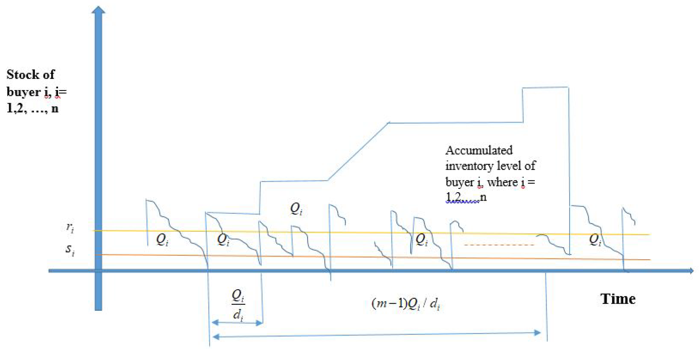
Each buyer in the SCM continuously reviews the inventory level. As a result, ( q i ) order is placed by buyer i only when the level of inventory reaches to a specified indicator that is the reorder point ( r i ) (see Figure 1). Therefore, the approximated average inventory for buyer i over the time cycle is given by
q i 2 + r i d i L i .
Now, the reorder point r i can be expressed as d i L i + k i σ i L i , which results in the average inventory for the i-th buyer being
q i 2 + k i σ i t s i + q i P
Hence, the holding cost for buyer i per unit time is
h b i q i 2 + k i σ i t s i + q i P .
Shortage cost.
As the production machine produces defective items in the long-run, shortages must occurs, the backorder quantity for buyers are E ( x 1 i r 1 i ) + and E ( x 2 i r 2 i ) + ., then the shortage cost per item per unit time is given by
d i π i q i E ( x 1 i r 1 i ) + + d i π i ( m 1 ) q i E ( x 2 i r 2 i ) + .
Transportation cost.
The cost for transportation of buyers is given by
m C T i d i q i .
Lead time crashing cost.
Some of the most realistic research these days is to satisfy customers by reducing the lead time when an extra cost is added by the production manager. The lead time can be reduced in two ways, by reducing production and transportation time. According to the assumptions, the lead time crashing cost per unit time can be expressed as
m d i C R i ( t s i ) q i
The total expected cost for buyer i is T E C b i = ordering cost + holding cost + shortage cost + transportation cost + lead time crashing cost
Thus, T E C b i leads to the following expression:
T E C b i ( q i , k i , L i ) = [ A 0 b i e r i I b i d i q i + I b i d i q i + h b i q i 2 + k i σ i t s i + q i P + d i π i q i E ( x 1 i r 1 i ) + + d i π i ( m 1 ) q i E ( x 2 i r 2 i ) + + m d i C T i q i + m d i C R i ( t s i ) q i ] .
For the distribution-free approach, a lemma was proved by Gallego and Moon [47], in which they proved that “if the distribution G of demand D is unknown, then,
E ( D Q ) + [ σ 2 + ( Q μ ) 2 ] 1 2 ( Q μ ) 2 .
The above expression is tight for every Q if there exist a distribution G * ζ , where ζ is the worst possible distribution.
According to Gallego and Moon’s [47], lemma where the least favorable distribution G ζ , one can obtain
E ( x 1 i R 1 i ) + σ i 2 L i ( P , q i ) + ( R 1 + i d i L i ( P , q i ) ) 2 ( R 1 i d i L i ( P , q i ) ) 2 = σ i 2 t s + q i P [ 1 + k 1 i 2 k 1 i ]
E ( x 2 i R 2 i ) + σ i 2 L i ( t T i ) + ( R 2 i d i L i ( t T i ) ) 2 ( R 2 i d i L i ( t T i ) ) 2 = σ i 2 t T i 1 + k 1 i 2 t s i + q i P t T i k 1 i t s i + q i P t T i .
Then, Equation (1) can be rewritten as
T E C b i ( Q , k i , P , m , I b i ) = [ d i q i A 0 b i e r i I b i + I b i + m C T i + h b i q i 2 + k i σ i t s i + q i P + d i π i σ i 2 q i t s + q i P [ 1 + k 1 i 2 k 1 i ] + m d i C R i ( t s i ) q i + d i π i σ i ( m 1 ) 2 q i t T i 1 + k 1 i 2 t s i + q i P t T i k 1 i t s i + q i P t T i ]
T E C b i ( Q , k i , P , m , I b i ) = [ d i q i A 0 b i e r i I b i + I b i + m C T i + h b i q i 2 + k i σ i t s i + q i P + d i π i q i ( σ i 2 t s + q i P [ 1 + k 1 i 2 k 1 i ] + m C R i ( t s i ) π i + σ i ( m 1 ) 2 t T i 1 + k 1 i 2 t s i + q i P t T i k 1 i t s i + q i P t T i ) ] .

3.2. Mathematical Model for the Vendor

To fulfill the buyer’s demand, the vendor produces Q quantity at a production rate P and the production cost C v ( P ) . As it is too difficult to guess how much production is needed, in this model, a variable production rate P with the variable production cost C v ( P ) is considered for the vendor. The vendor uses a single-setup-multi-delivery (SSMD) policy to transport the items to each buyer. Thus m shipment is considered for a single-setup-multi-delivery (SSMD) policy. Thus the total cycle time for vendor is m Q D . Two continuous investments are considered by the vendor to reduce the total system cost. An investment A v is used to reduce the setup cost of the vendor and another investment θ is used to reduce the chance of a system out-of-control state from in-control state. As in long-run system, the production process may move from an in-control to out-of-control state due to the labour problems, machinery problems etc. To reduce this chance, a continuous investment θ is introduced by the vendor. In this model, the following costs component are used for vendor:
Setup cost with an investment.
The setup cost for the vendor per unit time is D A v m Q . But a continuous investment is introduced to reduce the setup cost. Hence, after introducing continuous investment, the total setup cost for the vendor is given by
b ln A v 0 A v + A v D m Q
Holding cost.
The average inventory of the vendor is
m Q Q P + ( m 1 ) Q D m 2 Q 2 2 P Q 2 D ( 1 + 2 + + ( m 1 ) ) D m Q = Q 2 m 1 D P 1 + 2 D P .
(see Figure 2)
Therefore, the holding cost per unit time for the vendor is
h v Q 2 m 1 D P 1 + 2 D P .
Investment.
To improve the quality of the product, the vendor uses some investment. Thus, the investment for quality improvement is given by
B ln θ 0 θ .
Total investment.
Thus, the total investment for the reduced setup cost and improved the quality of the product is given by:
b ln A v 0 A v + B ln θ 0 θ = γ B ln θ b ln A v where , γ = B ln θ 0 + b ln A v 0 and 0 < θ θ 0 , 0 < A v A v 0 .
Production/material cost.
Production cost C v ( P ) of the vendor assumed to be a function of P. The production cost is of the form is:
C v ( P ) = ζ 1 P + ζ 2 P .
The unit production cost is P * = ζ 2 ζ 1 Therefore, the total expected cost of to the vendor is expressed as T E C v = setup cost + holding cost + material cost + investment cost i.e.,
T E C v ( m , Q , P , A v , θ ) = A v D m Q + Q 2 h v m 1 D P 1 + 2 D P + C v ( P ) D + S D m Q θ 2 + β γ B ln θ b ln A v .
In order to obtain centralized decisions for both the vendor and buyers to minimize the entire supply chain cost, the total cost expression of both ends must be combined. Therefore, the joint total expected cost for both vendor and the buyers ( J T E C ) is obtained as follows
J T E C ( Q , k i , m , θ , P , I , A v ) = i = 1 n [ D Q A 0 b i e r i I b i + I b i + A v m + m C T i + h b i Q 2 D d i + k i σ i t s i + Q P + D π i Q ( σ i 2 t s + q i P [ 1 + k 1 i 2 k 1 i ] + m C R i ( t s i ) π i + σ i ( m 1 ) 2 t T i [ 1 + k 1 i 2 t s i + q i P t T i k 1 i t s i + q i P t T i ] ) ] + Q 2 h v m 1 D P 1 + 2 D P + D C v ( P ) + S D m Q θ 2 + β γ B ln θ b ln A v .

4. Solution Methodology

The main aim of this model is to minimize the optimum value of the decision variable such as the total joint cost can be minimized. This is an unconstrainted minimization problem along with an integer programming problem. To find the optimum values of decision variable one needs to calculate the first order derivative of the objective function with respect to the decision variables and then equate them to zero. Now, according to the assumptions, m is an integer and therefore, can be treated as a discrete decision variable. One can use the analytic discrete optimization method to find the optimum value of m.
To find the optimum value of the other decision variables, one can use the classical optimization technique, which gives the global optimum value. To do this, after calculating derivatives with respect to k i , θ , I, A v , Q and P, one can obtain
J T E C ( Q , k , m , θ , P , I , A v ) k i = i = 1 n q i P + t s i σ i [ h b i + d i π i 2 q i { k i 1 + k i 2 1 + ( m 1 ) k i ( t s i + q i P ) t T i + ( t s i + q i P ) k i 2 1 } ] ,
J T E C ( Q , k , m , θ , P , I , A v ) k i = i = 1 n q i P + t s i σ i [ h b i + d i π i 2 q i { k i 1 + k i 2 1 + ( m 1 ) k i ( t s i + q i P ) t T i + ( t s i + q i P ) k i 2 1 } ] , J T E C ( Q , k , m , θ , P , I , A v ) θ = S D m Q 2 B β θ ,
J T E C ( Q , k , m , θ , P , I , A v ) I = ( 1 A v 0 r e r I ) D m Q , J T E C ( Q , k , m , θ , P , I , A v ) A v = D m Q b β A v , J T E C ( Q , k , m , θ , P , I , A v ) Q = τ 1 Q 2 + τ 2 Q + τ 3 , J T E C ( Q , k , m , θ , P , I , A v ) P = τ 4 P 2 + D ζ 2
(See Appendix A for the values of τ i , i = 1 , 2 , 3 , 4 .)
For a fixed positive integer m, the values of Q, k i , P, I, A v , and θ can be obtained by equating every individual equation of the system in Equation (5) to zero. Then, one can obtain the optimum result Q * , k i * , P * , I * , A v * and θ * as follows:
Q * = τ 1 τ 3 Q + τ 2 ,
k i * = m ( D π i 2 h b i Q ) D π i 1 1 + k i 2 + ( m 1 ) Q P + t s i t T i + Q P + t s i k i 2 ,
P * = τ 4 D ζ 2 ,
θ * = 2 B β S D m Q ,
I * = 1 r log ( r A v 0 ) ,
A v * = b m β Q D .
Lemma 1.
For the fixed value of m, the condition is sufficient at the optimum value of the decision variables Q * , k i * , P * , I * , A v * and θ * , i.e., all principal minor of the Hessian matrix is greater than zero for the optimum value of the decision variables Q * , k i * , P * , I * , A v * and θ * .
Proof. 
See Appendix B for the proof of the lemma. □

Solution Algorithm

A closed form solution of this mathematical model is very difficult to obtain. One can use the fixed point iteration technique to create a suitable algorithm in order to solve the model.
Step 1
Set m = 1 , and input all the values of the parameters.
Step 2
For all buyers i = 1 , 2 , , n , assign the values of all parameters and perform the following steps.
Step 3
For every combination of L i , r , r = 1 , 2 , , N i , i = 1 , 2 , , n perform steps 3a–3e.
Step 3a
Set k i j 1 = 0 for each buyer i.
Step 3b
Substitute k i j 1 , (i = 1,2,...,n) into Equation (6) and evaluate Q j 1 .
Step 3c
Utilize Q j 1 to determine the value of ( k i j 2 ) for each i from (7).
Step 3d
Using the value of ( k i j 2 ) , obtain the value of k i j 2 from the normal distribution table.
Step 3e
Repeat steps 3b to 3d until no changes occur in the values of Q j and k i j and denote these values as Q j * and k i j * , respectively.
Step 4
Evaluate the value of P j * , I j * , θ j * , and A v j * from Equations (8), (10), (9), and (11), respectively, using the value of Q j * .
Step 5
Denote the latest updated values of Q j , k i j , P j , I θ j , and A v j as Q j * * , k i j * * , P j * * I j * * , θ j * * , and A v j * * respectively.
Step 6
Obtain J T E C ( Q j * * , k i j * * , P j * * , I j * * , θ j * * , A v j * * , m ) and
M i n j = 1 , 2 , . . . , N i J A T C ( Q j * * , k i j * * , P j * * , I j * * , θ j * * , A v j * * , m ) for all i.
Step 7
Set m = m + 1 .
If J T E C ( Q m * * , k i m * * , P m * * , I m * * , θ m * * , A v m j * * , m ) J A T C ( Q m 1 * * , k m 1 * * , I m 1 * * , θ m 1 * * , A v m 1 , m 1 ) , repeat steps 2–4. Otherwise, go to Step 6.
Step 8
Set J T E C ( Q m * * , k m * * , I m * * , θ m * * , A v * * , m ) = J T E C ( Q m 1 * * , k m 1 * * , S m 1 * * , θ m 1 * * , A v m 1 * * , m 1 ) .
Then, ( Q * * , k * * , L * * , I * * , θ * * , A v * * , m * * ) is the optimal solution.

5. Numerical Analysis

In this section, some numerical examples are provided to validate the model. The parametric values of demand, holding cost, initial ordering cost, stockout cost, marginal profit, annual fractional cost for three different buyer’s are given in Table 2, and parametric values for the vendor are given in Table 3. The parametric values are taken from Majumder et al. [14]. By using the software Matlab R2015a, one can obtain the optimum results which are shown in Table 4.
From Table 4, one can easily find that the total system cost is minimized when the batch size is 4, which can be obtained by analytic discrete optimization technique, the optimum quantity is 595.65 units, the investment for reducing setup cost per unit is 253.13 ($/order), the optimum production rate is 704.48 , the optimum setup cost is 1152.89 ($/setup) and the optimum production cost per unit is 2.34 ($/unit). Using those optimum values, the total system cost was $ 2225.18 .
Based on the above results this model is more beneficial compared to the Sarkar and Majumder [10], Sarkar and Moon [42], and Kim and Sarkar’s [48] model. In Sarkar and Majumder’s [10] model, the total system cost was $ 6994.4 , in Sarkar and Moon’s [42] model the total system cost was $ 3500.73 , whereas in Kim and Sarkar’s [48] model this total system cost was $ 1961.21 , with a constant production rate, but in this current model the production rate is variable.

5.1. Special Case I: When No Investment Is Used

When there is no investment, that is I = 0 , then the total system cost T E C is $ 179162813414.03 . It is found that without investment, the system cost is huge compared to the use of investment. Thus, if one uses investment then the total system cost is remarkably reduced.

5.2. Special Case II: When No Quality Improvement Is Considered

If θ = 0 , that is the probability of the production process which may go to an out-of-control state is zero, then the system cost T E C is $ 5928.30 , thus the investment for reducing the probability of the production process, which may go to an out-of-control state is also reduces the total system cost.

5.3. Special Case III: When Setup Cost Is Fixed

If the setup cost is fixed, then the total system cost T E C is $ 404516898.87 . Thus, it is clear that use of investment to reduce setup cost and is highly beneficial to any industry.

6. Sensitivity Analysis

One can easily find the effect of a change of parameters to the total cost by the sensitivity shown in Table 5. This table is formulated for a change in parameter 10 % , 5 % , 5 % , and 10 % . From Table 5, it is easily concluded that
  • A small change in ordering cost for buyers has a great effect in total cost of the SCM system.
  • A small change in the initial setup cost also has an impact on total cost. Setup cost is more effective for this model. With very little change in setup cost, there is a huge change in total cost. From the sensitivity table it is clear that setup cost is more sensitive for this model.
  • Scaling parameter B is lightly sensitive for the total cost in this model.
The effect of change in total cost are shown graphically in the Figure 3, Figure 4 and Figure 5.

Case Study

A real case study was also done to validate this model. The model was tested on real data from a company, located in West Bengal, India. They happily accepted the proposal to allow access to data from their company and the model is validated with the real data. The results were found in the similar direction of the research. The results of the proposed model with the real data were considered after the normalization of each data, as without normalization, those data cannot fit with the proposed model. The basic normalization towards mean was used for the purpose. Using sample mean, sample variance, and histogram, and finally the confirmation test of the distribution function. The input data from the company is given in Table 6 and Table 7 and the results are given in Table 8. The company was really satisfied with results. But if they will use the findings of the proposed model. Thus, the proposed strategy effects a major savings of the company. Based on the findings, the company may change their production planning.

7. Managerial Insights

This model developed a single vendor-multi-buyer SCM model, where the single vendor produces a single item and sends it to multiple buyers using a SSMD policy. The production rate and production cost are variable which is quite realistic. Three types of investments are used to reduce cost and improve the quality of the production system. Based on different variables such as lead time, order quantity, reorder point, production cost, production rate, and number of shipments, investments decision are made. The managerial insights for this model are as follows:
  • The production rate are considered as variable, which is more realistic rather than constant. Industries can use variable production for cost savings or earning more profit.
  • The production cost is also variable which also a more realistic.
  • The company would like to reduce the total cost of their production system. For this, a continuous investment is made to reduce the setup cost of whole production system along with a discrete investment to reduce the ordering cost.
  • To control the long-run system, a continuous investment is made such that the production quality can be improved.
  • By increasing the lead time crashing cost, a manager can reduce the lead time to upgrade the service label for the customer.

8. Concluding Remarks

This research developed an SCM model, where a single vendor produces a single type of item and sends it to multiple buyers using an SSMD policy. Contradictory to the literature, a variable production rate with variable production cost was used. The production cost depends on the production rate. From the numerical result, it is found that the optimum result is obtained when the number of shipments is four. It is also concluded that some investment in setup cost, reduced the setup cost of the whole system and some investment was done to improve the quality of the production system for the long run. As this model considered defective items, the inspection process (see for reference Sarkar [49]) will be a very interesting finding as a future extension. This model can also be extended by considering the autonomation policy for inspection along with different types of warehousing. This model can be extended in future with unreliability for the vendor. Another very interesting extension of this model would be considering a multi-echelon model with multi-buyer and multi-vendor for multiple product or an assembled product.

Author Contributions

Conceptualization, B.S.; methodology, B.S. and B.K.D.; software, B.K.D.; validation, B.S., B.K.D. and S.P.; formal analysis, B.K.D; investigation, B.S.; resources, B.S. and S.P.; data curation, B.K.D., B.S. and S.P.; writing—original draft preparation, B.K.D.; writing—review and editing, B.S., B.K.D., S.P.; visualization, B.S., and B.K.D.; supervision, S.P., and B.S.

Acknowledgments

This research was supported by Basic Science Research Program through the National Research Foundation of Korea (NRF) funded by the Ministry of Education, Science and Technology (Project Number: 2017R1D1A1B03033846).

Conflicts of Interest

The authors declare no conflict of interest.

Appendix A

τ 1 = D ( A 0 b i e r i I b i + A v m + m C T i + I b i ) + i = 1 n d i π i σ i [ m C R i ( t s i ) π i σ i + 1 2 q i P + t s i 1 + k i 2 k i + 1 2 ( m 1 ) t T i + ( q i P + t s i ) k i 2 q i P + t s i ] τ 2 = i = 1 n d i π i σ i 4 P 1 + k i 2 k i q i P + t s i + ( m 1 ) k i k i t T i + ( q i P + t s i ) k i 2 1 q i P + t s i τ 3 = i = 1 n h b i d i 2 D + k i σ i 2 P q i P + t s i + 1 2 m S θ D + 1 2 h v 2 D P + m 1 D P 1 τ 4 = [ D ζ 1 h v Q D ( m 2 ) 2 + D π i σ i k i 2 ( m 1 ) 4 t T i + Q P + t s i k i 2 + σ i 2 Q P + t s i h b i Q k i D π i 2 ( k i m 1 + k i 2 ) ]

Appendix B

Proof of Lemma 1
This paper computes the Hessian matrix at the optimal values for a given m as follows:
| H ( J T E C ) | = 2 J T E C ( . ) I 2 2 J T E C ( . ) I θ 2 J T E C ( . ) I A v 2 J T E C ( . ) Q P 2 J T E C ( . ) I k 2 J T E C ( . ) I Q 2 J T E C ( . ) θ I 2 J T E C ( . ) θ 2 2 J T E C ( . ) θ A v 2 J T E C ( . ) θ P 2 J T E C ( . ) θ k 2 J T E C ( . ) θ Q 2 J T E C ( . ) A v I 2 J T E C ( . ) A v θ 2 J T E C ( . ) A v 2 2 J T E C ( . ) A v P 2 J T E C ( . ) A v k 2 J T E C ( . ) A v Q 2 J T E C ( . ) P I 2 J T E C ( . ) P θ 2 J T E C ( . ) P A v 2 J T E C ( . ) P 2 2 J T E C ( . ) P k 2 J T E C ( . ) P Q 2 J T E C ( . ) k I 2 J T E C ( . ) k θ 2 J T E C ( . ) k A v 2 J T E C ( . ) k P 2 J T E C ( . ) k 2 2 J T E C ( . ) k Q 2 J T E C ( . ) Q I 2 J T E C ( . ) Q θ 2 J T E C ( . ) Q A v 2 J T E C ( . ) Q P 2 J T E C ( . ) Q k 2 J T E C ( . ) Q 2
where J T E C ( . ) = J T E C ( Q , k , θ , P , I , A v ) .
The second order partial derivatives at the optimal values are
2 J T E C ( . ) Q 2 = 2 τ 1 Q 3 τ 2 Q 2 2 J T E C ( . ) P 2 = 2 τ 4 P 3 2 J T E C ( . ) I 2 = A 0 b i r 2 I e r I Q 2 J T E C ( . ) θ 2 = B β θ 2 2 J T E C ( . ) A v 2 = b β A v 2 2 J T E C ( . ) Q I = 2 J T E C ( . ) I Q = ( 1 A 0 b i r e r I ) D Q 2
2 J T E C ( . ) K 2 = 1 2 D π i σ i Q P + t s i [ 1 1 + k i 2 3 2 + ( m 1 ) Q P + t s i t T i + Q P + t s i k i 2 ( 1 Q P + t s i k i 2 t T i + Q P + t s i k i 2 ) ] 2 J T E C ( . ) Q P = 2 J T E C ( . ) P Q = 1 2 h v ( 2 D P 2 + m D P 2 ) + h b i Q k i σ i 4 P 3 ( Q P + t s i ) 3 2 k i σ i 2 P 2 Q P + t s i + 1 Q D π i ( Q ( k i + 1 + k i 2 ) σ i 8 P 3 ( Q P + t s i ) 3 2 ( k i + 1 + k i 2 ) σ 4 P 2 Q P + t s i + 1 2 ( m 1 ) t T i ( Q k i 4 P 3 ( Q P + t s i t T i ) 3 2 t T i 2 + k i 2 P 2 Q P + t s i t T i t T i + Q k i 4 4 P 3 t T i 2 ( 1 + ( Q P + t s i ) k i 2 t T i ) 3 2 k i 2 2 P 2 t T i 1 + ( Q P + t s i ) k i 2 t T i ) σ i ) D π i Q ( k i + 1 + k i 2 ) σ i 4 P 2 Q P + t s i + 1 2 ( m 1 ) t T i Q k i 2 P 2 Q P + t s i t T i t T i Q k i 2 2 P 2 t T i 1 + ( Q P + t s i ) k i 2 t T i σ i Q 2
2 J T E C ( . ) Q θ = 2 J T E C ( . ) θ Q = m S D 2 2 J T E C ( . ) Q A v = 2 J T E C ( . ) A v Q = D m Q 2 2 J T E C ( . ) P k = 2 J T E C ( . ) k P = 1 2 P 2 [ h b i Q σ i Q P + t s i + D π i σ i [ k i 1 + k i 2 1 2 Q P + t s i + ( m 1 ) 1 2 Q P + t s i + ( Q P + t s i ) k i 2 2 t T i + ( Q P + t s i ) k i 2 3 2 k i t T i + ( Q P + t s i ) k i 2 ] ] 2 J T E C ( . ) P I = 2 J T E C ( . ) I P = 0 2 J T E C ( . ) P θ = 2 J T E C ( . ) θ P = 0 2 J T E C ( . ) P A v = 2 J T E C ( . ) A v P = 0 2 J T E C ( . ) k I = 2 J T E C ( . ) I k = 0 2 J T E C ( . ) k θ = 2 J T E C ( . ) θ k = 0 2 J T E C ( . ) k A v = 2 J T E C ( . ) A v k = 0
2 J T E C ( . ) Q k = 2 J T E C ( . ) k Q = h b i σ i 2 P Q P + t + 1 Q D π i ( ( k i 1 + k i 2 1 ) σ i 4 P Q P + t s i + 1 2 ( m 1 ) t T i 1 2 P Q P + t s i t T i t T i ( Q P + t s i ) k i 3 2 P t T i 2 ( 1 + ( Q P + t s i ) k i 2 t T i ) 3 2 + k i P t T i 1 + ( Q P + t ) k i 2 t T i σ i ) D π i 1 2 Q P + t s i ( 1 + k i 1 + k i 2 ) σ i + 1 2 ( 1 + m ) t T i ( Q P + t s i t T i + ( Q P + t ) α t T i 1 + ( Q P + t s i ) k i 2 t T i ) σ i Q 2 2 J T E C ( . ) I θ = 2 J T E C ( . ) θ I = 0 2 J T E C ( . ) I A v = 2 J T E C ( . ) A v I = 0 2 J T E C ( . ) θ A v = 2 J T E C ( . ) A v θ = 0
Now, the first order principal minor at the optimal vales is given by
d e t ( H 11 ) = d e t 2 J T E C ( . ) I 2 = A 0 b i r 2 I b i e r I b i Q > 0 .
The first principal minor is grater than zero since all the parameters and variables are positive:
The second order principal minor of H ( J T E C ) is
det ( H 22 ) = det 2 J T E C ( . ) I 2 2 J T E C ( . ) I θ 2 J T E C ( . ) I θ 2 J T E C ( . ) θ 2 = A 0 b i r 2 I b i e r I b i Q B β θ 2 0 > 0
The second principal minor is also grater then zero as 2 J T E C ( . ) I 2 > 0 , 2 J T E C ( . ) θ 2 > 0 , and 2 J T E C ( . ) I θ = 0 .
The third order principal minor of H ( J T E C ) is given by
det ( H 33 ) = det 2 J T E C ( . ) I 2 2 J T E C ( . ) I θ 2 J T E C ( . ) I A v 2 J T E C ( . ) θ I 2 J T E C ( . ) θ 2 2 J T E C ( . ) θ A v 2 J T E C ( . ) I A v 2 J T E C ( . ) A v θ 2 J T E C ( . ) A v 2 = A 0 b i r 2 I b i e r I b i Q B β θ 2 b β A v 2 > 0 .
Thus, third principal minor is also grater than zero, as all three terms 2 J T E C ( . ) I 2 , 2 J T E C ( . ) θ 2 , 2 J T E C ( . ) A v 2 are positive and others terms are zero.
The forth order principal minor of H ( J T E C ) is
det ( H 44 ) = 2 J T E C ( . ) I 2 2 J T E C ( . ) I θ 2 J T E C ( . ) I A v 2 J T E C ( . ) I P 2 J T E C ( . ) I θ 2 J T E C ( . ) θ 2 2 J T E C ( . ) θ A v 2 J T E C ( . ) θ P 2 J T E C ( . ) A v I 2 J T E C ( . ) θ A v 2 J T E C ( . ) A v 2 2 J T E C ( . ) A v P 2 J T E C ( . ) P I 2 J T E C ( . ) P θ 2 J T E C ( . ) P A v 2 J T E C ( . ) P 2 = A 0 b i r 2 I b i e r I b i Q B β θ 2 b β A v 2 2 τ 4 P 3 > 0 .
Thus fourth principal minor is grater than zero as all four terms are positive and all others terms are zero.
The fifth order principal minor of H ( J T E C ) is given by
det ( H 55 ) = det 2 J T E C ( . ) I 2 2 J T E C ( . ) I θ 2 J T E C ( . ) I A v 2 J T E C ( . ) I P 2 J T E C ( . ) I k 2 J T E C ( . ) I θ 2 J T E C ( . ) θ 2 2 J T E C ( . ) θ A v 2 J T E C ( . ) θ P 2 J T E C ( . ) θ k 2 J T E C ( . ) A v I 2 J T E C ( . ) θ A v 2 J T E C ( . ) A v 2 2 J T E C ( . ) A v P 2 J T E C ( . ) A v k 2 J T E C ( . ) P I 2 J T E C ( . ) P θ 2 J T E C ( . ) P A v 2 J T E C ( . ) P 2 2 J T E C ( . ) P k 2 J T E C ( . ) k I 2 J T E C ( . ) k θ 2 J T E C ( . ) k A v 2 J T E C ( . ) P k 2 J T E C ( . ) k 2 .
= A 0 b i r 2 I b i e r I b i Q B β θ 2 b β A v 2 det 2 J T E C ( . ) P 2 2 J T E C ( . ) P k 2 J T E C ( . ) k P 2 J T E C ( . ) k 2 .
Now, if
2 τ 4 P 3 > 1 2 P 2 [ h b i Q σ i Q P + t s i + D π i σ i [ k i 1 + k i 2 1 2 Q P + t s i + ( m 1 ) 1 2 Q P + t s i + ( Q P + t s i ) k i 2 2 t T i + ( Q P + t s i ) k i 2 3 2 k i t T i + ( Q P + t s i ) k i 2 ] ]
1 2 D π i σ i Q P + t s i 1 1 + k i 2 3 2 + ( m 1 ) Q P + t s i t T i + Q P + t s i k i 2 1 Q P + t s i k i 2 t T i + Q P + t s i k i 2 > 1 2 P 2 [ h b i Q σ i Q P + t s i + D π i σ i [ k i 1 + k i 2 1 2 Q P + t s i + ( m 1 ) 1 2 Q P + t s i + ( Q P + t s i ) k i 2 2 t T i + ( Q P + t s i ) k i 2 3 2 k i t T i + ( Q P + t s i ) k i 2 ] ] ,
then by the formula x y > z 2 , if x > z , and y > z , one can get
det 2 J T E C ( . ) P 2 2 J T E C ( . ) P k 2 J T E C ( . ) k P 2 J T E C ( . ) k 2 = 2 J T E C ( . ) P 2 × 2 J T E C ( . ) k 2 2 J T E C ( . ) k P 2 > 0 .
Thus, one can state that fifth order principal minor is grater than zero as this is the products of four positive terms and all others terms are zero. Now, the sixth order minor i.e., the full Hessian is of the form
| H 66 | = 2 J T E C ( . ) I 2 2 J T E C ( . ) I θ 2 J T E C ( . ) I A v 2 J T E C ( . ) Q P 2 J T E C ( . ) I k 2 J T E C ( . ) I Q 2 J T E C ( . ) θ I 2 J T E C ( . ) θ 2 2 J T E C ( . ) θ A v 2 J T E C ( . ) θ P 2 J T E C ( . ) θ k 2 J T E C ( . ) θ Q 2 J T E C ( . ) A v I 2 J T E C ( . ) A v θ 2 J T E C ( . ) A v 2 2 J T E C ( . ) A v P 2 J T E C ( . ) A v k 2 J T E C ( . ) A v Q 2 J T E C ( . ) P I 2 J T E C ( . ) P θ 2 J T E C ( . ) P A v 2 J T E C ( . ) P 2 2 J T E C ( . ) P k 2 J T E C ( . ) P Q 2 J T E C ( . ) k I 2 J T E C ( . ) k θ 2 J T E C ( . ) k A v 2 J T E C ( . ) k P 2 J T E C ( . ) k 2 2 J T E C ( . ) k Q 2 J T E C ( . ) Q I 2 J T E C ( . ) Q θ 2 J T E C ( . ) Q A v 2 J T E C ( . ) Q P 2 J T E C ( . ) Q k 2 J T E C ( . ) Q 2
= 2 J T E C ( . ) I 2 × 2 J T E C ( . ) θ 2 2 J T E C ( . ) θ A v 2 J T E C ( . ) θ P 2 J T E C ( . ) θ k 2 J T E C ( . ) θ Q 2 J T E C ( . ) A v θ 2 J T E C ( . ) A v 2 2 J T E C ( . ) A v P 2 J T E C ( . ) A v k 2 J T E C ( . ) A v Q 2 J T E C ( . ) P θ 2 J T E C ( . ) P A v 2 J T E C ( . ) P 2 2 J T E C ( . ) P k 2 J T E C ( . ) P Q 2 J T E C ( . ) k θ 2 J T E C ( . ) k A v 2 J T E C ( . ) k P 2 J T E C ( . ) k 2 2 J T E C ( . ) k Q 2 J T E C ( . ) Q θ 2 J T E C ( . ) Q A v 2 J T E C ( . ) Q P 2 J T E C ( . ) Q k 2 J T E C ( . ) Q 2 2 J T E C ( . ) I Q × | H 55 | .
Now, one have to calculate
2 J T E C ( . ) I 2 × 2 J T E C ( . ) θ 2 × 2 J T E C ( . ) A v 2 2 J T E C ( . ) A v P 2 J T E C ( . ) A v k 2 J T E C ( . ) A v Q 2 J T E C ( . ) P A v 2 J T E C ( . ) P 2 2 J T E C ( . ) P k 2 J T E C ( . ) P Q 2 J T E C ( . ) k A v 2 J T E C ( . ) k P 2 J T E C ( . ) k 2 2 J T E C ( . ) k Q 2 J T E C ( . ) Q A v 2 J T E C ( . ) Q P 2 J T E C ( . ) Q k 2 J T E C ( . ) Q 2
2 J T E C ( . ) A v 2 2 J T E C ( . ) A v P 2 J T E C ( . ) A v k 2 J T E C ( . ) A v Q 2 J T E C ( . ) P A v 2 J T E C ( . ) P 2 2 J T E C ( . ) P k 2 J T E C ( . ) P Q 2 J T E C ( . ) k A v 2 J T E C ( . ) k P 2 J T E C ( . ) k 2 2 J T E C ( . ) k Q 2 J T E C ( . ) Q A v 2 J T E C ( . ) Q P 2 J T E C ( . ) Q k 2 J T E C ( . ) Q 2 = 2 J T E C ( . ) A v 2 × 2 J T E C ( . ) P 2 2 J T E C ( . ) P k 2 J T E C ( . ) P Q 2 J T E C ( . ) k P 2 J T E C ( . ) k 2 2 J T E C ( . ) k Q 2 J T E C ( . ) Q P 2 J T E C ( . ) Q k 2 J T E C ( . ) Q 2 + D m Q 2 × 2 J T E C ( . ) P A v 2 J T E C ( . ) P 2 2 J T E C ( . ) P k 2 J T E C ( . ) k A v 2 J T E C ( . ) k P 2 J T E C ( . ) k 2 2 J T E C ( . ) Q A v 2 J T E C ( . ) Q P 2 J T E C ( . ) Q k .
Now, from the previous argument one can find that
2 J T E C ( . ) P 2 2 J T E C ( . ) P k 2 J T E C ( . ) P Q 2 J T E C ( . ) k P 2 J T E C ( . ) k 2 2 J T E C ( . ) k Q 2 J T E C ( . ) Q P 2 J T E C ( . ) Q k 2 J T E C ( . ) Q 2 > 0 and , 2 J T E C ( . ) P A v 2 J T E C ( . ) P 2 2 J T E C ( . ) P k 2 J T E C ( . ) k A v 2 J T E C ( . ) k P 2 J T E C ( . ) k 2 2 J T E C ( . ) Q A v 2 J T E C ( . ) Q P 2 J T E C ( . ) Q k > 0 .
Hence | H 66 | > 0 , since 2 J T E C ( . ) I 2 > 0 , 2 J T E C ( . ) I Q < 0 , and | H 55 | > 0 . Thus, sixth principal minor | H 66 | is greater then zero as this is the sum of positive terms.
Hence one can state that all principal minor that is | H 11 | , | H 22 | , | H 33 | , | H 44 | , | H 55 | , | H 66 | are grater than zero for the optimal values of the decision variables, which is the sufficient condition for the global optimum result of this model.
Hence the Lemma 1 is proved.

References

  1. Taft, E.W. The most economical production lot. Iron Age 1918, 101, 1410–1412. [Google Scholar]
  2. Cárdenas-Barrón, L.E.; Chung, K.J.; Treviño-Garza, G. Celebrating a century of the economic order quantity model in honor of Ford Whitman Harris. Int. J. Prod. Econ. 2014, 155, 1–7. [Google Scholar]
  3. Sarkar, B. A production-inventory model with probabilistic deterioration in two-echelon supply chain management. Appl. Math. Model. 2013, 37, 3138–3151. [Google Scholar] [CrossRef]
  4. Goyal, S.K. An integrated inventory model for a single supplier-single customer problem. Int. J. Prod. Res. 1976, 15, 107–111. [Google Scholar] [CrossRef]
  5. Banerjee, A. A joint economic-lot-size model for purchaser and vendor. Decis. Sci. 1986, 17, 292–311. [Google Scholar] [CrossRef]
  6. Goyal, S.K. Economic ordering policy for deteriorating items over an infinite time horizon. Eur. J. Oper. Res. 1987, 28, 298–301. [Google Scholar] [CrossRef]
  7. Chakraborty, D.; Bhuiya, S.K. A Continuous Review Inventory Model with Fuzzy Service Level Constraint and Fuzzy Random Variable Parameters. Int. J. Appl. Comput. Math. 2017, 3, 3159–3174. [Google Scholar] [CrossRef]
  8. Ouyang, L.Y.; Yeh, N.C.; Wu, K.S. Mixture inventory model with backorders and lost sales for variable lead time. J. Oper. Res. Soc. 1996, 47, 829–832. [Google Scholar] [CrossRef]
  9. Ouyang, L.Y.; Wu, K.S.; Ho, C.H. Integrated vendor-buyer cooperative models with stochastic demand in controllable lead time. Int. J. Prod. Econ. 2004, 92, 255–266. [Google Scholar] [CrossRef]
  10. Sarkar, B.; Majumder, A. Integrated vendor-buyer supply chain model with vendor’s setup cost reduction. Appl. Math. Comput. 2013, 224, 362–371. [Google Scholar] [CrossRef]
  11. Moon, I.; Gallego, G. Distribution free procedures for some inventory models. J. Oper. Res. Soc. 1994, 45, 651–658. [Google Scholar] [CrossRef]
  12. Sarkar, B.; Majumder, A.; Sarkar, M.; Dey, B.K.; Roy, G. Two-echelon supply chain model with manufacturing quality improvement and setup cost reduction. J. Ind. Manag. Optim. 2017, 13, 1085–1104. [Google Scholar] [CrossRef] [Green Version]
  13. Dey, B.K.; Sarkar, B.; Sarkar, M.; Pareek, S. An integrated inventory model involving discrete setup cost reduction, variable safety factor, selling-price dependent demand, and investment. Rairo Oper. Res. 2019, 53, 39–57. [Google Scholar] [CrossRef]
  14. Majumder, A.; Jaggi, C.K.; Sarkar, B. A multi-retailer supply chain model with backorder and variable production cost. Rairo Oper. Res. 2018. [Google Scholar] [CrossRef]
  15. Banerjee, A.; Burton, J.S. Coordinated versus independent inventory replenishment policies for a vendor and multiple buyers. Int. J. Prod. Econ. 1994, 35, 215–222. [Google Scholar] [CrossRef]
  16. Banerjee, A.; Banerjee, S. A coordinated order-up-to inventory control policy for a single supplier and multiple buyers using electronic data interchange. Int. J. Prod. Econ. 1994, 35, 85–91. [Google Scholar] [CrossRef]
  17. Sarmah, S.P.; Acharya, D.; Goyal, S.K. Coordination of a single-manufacturer/multi-buyer supply chain with credit option. Int. J. Prod. Econ. 2008, 111, 676–685. [Google Scholar] [CrossRef]
  18. Khouja, M.; Mehrez, A. Economic production lot size model with variable production rate and imperfect quality. J. Oper. Res. Soc. 1994, 45, 1405–1417. [Google Scholar] [CrossRef]
  19. Tripathi, R.P.; Pareek, S.; Kaur, M. Inventory Model with Exponential Time-Dependent Demand Rate, Variable Deterioration, Shortages and Production Cost. Int. J. Appl. Comput. Math. 2017, 3, 1407–1419. [Google Scholar] [CrossRef]
  20. Chakrabarty, R.; Roy, T.; Chaudhuri, K.S. A Production: Inventory Model for Defective Items with Shortages Incorporating Inflation and Time Value of Money. Int. J. Appl. Comput. Math. 2017, 3, 195–212. [Google Scholar] [CrossRef]
  21. Hoque, M.A. Synchronization in the single-manufacturer multi-buyer integrated inventory supply chain. Eur. J. Oper. Res. 2008, 188, 811–825. [Google Scholar] [CrossRef]
  22. Jha, J.K.; Shanker, K. Two-echelon supply chain inventory model with controllable lead time and service level constraint. Comput. Ind. Eng. 2009, 57, 1096–1104. [Google Scholar] [CrossRef]
  23. Glock, C.H.; Kim, T. The effect of forward integration on a single-vendor–multi-retailer supply chain under retailer competition. Int. J. Prod. Econ. 2015, 164, 179–192. [Google Scholar] [CrossRef]
  24. Liao, C.J.; Shyu, C.H. An analytical determination of lead time with normal demand. Int. J. Oper. Prod. Manag. 1991, 11, 72–78. [Google Scholar] [CrossRef]
  25. Ben-Daya, M.; Raouf, A. Inventory models involving lead time as a decision variable. J. Oper. Res. Soc. 1994, 45, 579–582. [Google Scholar] [CrossRef]
  26. Pan, J.C.H.; Yang, J.S. A study of an integrated inventory with controllable lead time. Int. J. Prod. Res. 2002, 40, 1263–1273. [Google Scholar] [CrossRef]
  27. Annadurai, K.; Uthayakumar, R. Reducing lost-sales rate in (T,R,L) inventory model with controllable lead time. Appl. Math. Model. 2010, 34, 3465–3477. [Google Scholar] [CrossRef]
  28. Lo, S.T.; Wee, H.M.; Huang, W.C. An integrated production-inventory model with imperfect production processes and Weibull distribution deterioration under inflation. Int. J. Prod. Econ. 2007, 106, 248–260. [Google Scholar] [CrossRef]
  29. Huang, C.K.; Cheng, T.L.; Kao, T.C.; Goyal, S.K. An integrated inventory model involving manufacturing setup cost reduction in compound poisson process. Int. J. Prod. Res. 2011, 49, 1219–1228. [Google Scholar] [CrossRef]
  30. Tayyab, M.; Sarkar, B. Optimal batch quantity in a cleaner multi-stage lean production system with random defective rate. J. Clean. Prod. 2016, 139, 922–934. [Google Scholar] [CrossRef]
  31. Kang, C.W.; Ullah, M.; Sarkar, B.; Hussain, I.; Akhtar, R. Impact of random defective rate on lot size focusing work-in-process inventory in manufacturing system. Int. J. Prod. Res. 2017, 55, 1748–1766. [Google Scholar] [CrossRef]
  32. Mishra, U. An EOQ Model with Time Dependent Weibull Deterioration, Quadratic Demand and Partial Backlogging. Int. J. Appl. Comput. Math. 2017, 2, 545–563. [Google Scholar] [CrossRef]
  33. Khan, M.; Hussain, M.; Cárdenas-Barrón, L.E. Learning and screening errors in an EPQ inventory model for supply chains with stochastic lead time demands. Int. J. Prod. Res. 2017, 55, 4816–4832. [Google Scholar] [CrossRef]
  34. Chang, H.J.; Su, R.H.; Yang, C.T.; Weng, M.W. An economic manufacturing quantity model for a two-stage assembly system with imperfect processes and variable production rate. Comput. Ind. Eng. 2012, 63, 285–293. [Google Scholar] [CrossRef]
  35. Ca´rdenas-Barro´n, L.E.; Taleizadeh, A.A.; Treviño-Garza, G. An improved solution to replenishment lot size problem with discontinuous issuing policy and rework, and the multi-delivery policy into economic production lot size problem with partial rework. Expert Syst. Appl. 2012, 39, 13540–13546. [Google Scholar]
  36. Debata, S.; Acharya, M. An Inventory Control for Non-instantaneous Deteriorating Items with Non-zero Lead Time and Partial Backlogging Under Joint Price and Time Dependent Demand. Int. J. Appl. Comput. Math. 2017, 3, 1318–1393. [Google Scholar] [CrossRef]
  37. Sana, S.S.; Chaudhuri, K.S. An EMQ model in an imperfect production process. Int. J. Syst. Sci. 2010, 41, 635–646. [Google Scholar] [CrossRef]
  38. Wee, H.M.; Wang, W.T.; Cárdenas-Barrón, L.E. An alternative EPQ model with rework process at a single-stage manufacturing system with planned backorders. Comput. Ind. Eng. 2013, 64, 748–755. [Google Scholar] [CrossRef]
  39. Sarkar, B.; Cárdenas-Barrón, L.E.; Sarkar, M.; Singgih, M.L. An economic production quantity model with random defective rate, rework process and backorders for a single stage production system. J. Manuf. Syst. 2014, 33, 423–435. [Google Scholar] [CrossRef]
  40. Das Roy, M.; Sana, S.S.; Chaudhuri, K.S. An integrated producer–buyer relationship in the environment of EMQ and JIT production systems. Int. J. Prod. Res. 2012, 50, 5597–5614. [Google Scholar]
  41. Kim, M.; Kim, J.; Sarkar, B.; Sarkar, M.; Iqbal, M.W. An improved way to calculate imperfect items during long-run production in an integrated inventory model with backorders. J. Manuf. Syst. 2018, 47, 153–167. [Google Scholar] [CrossRef]
  42. Sarkar, B.; Moon, I. Improved quality, setup cost reduction, and variable backorder costs in an imperfect production process. Int. J. Prod. Econ. 2014, 155, 204–213. [Google Scholar] [CrossRef]
  43. Cárdenas-Barrón, L.E.; Sarkar, B.; Treviño-Garza, G. An improved solution to the replenishment policy for the EMQ model with rework and multiple shipments. Appl. Math. Model. 2013, 37, 5549–5554. [Google Scholar]
  44. Pal, B.; Sana, S.S.; Chaudhuri, K. A mathematical model on EPQ for stochastic demand in an imperfect production system. J. Manuf. Syst. 2013, 32, 260–270. [Google Scholar] [CrossRef]
  45. Sana, S.S. An EOQ model for stochastic demand for limited capacity of own warehouse. Ann. Oper. Res. 2015, 233, 383–399. [Google Scholar] [CrossRef]
  46. Pal, B.; Sana, S.S.; Chaudhuri, K. A distribution-free newsvendor problem with nonlinear holding cost. Int. J. Syst. Sci. 2015, 46, 1209–1277. [Google Scholar] [CrossRef]
  47. Gallego, G.; Moon, I. The Distribution free Newsboy problem: Review and extensions. J. Oper. Res. Soc. 1993, 44, 825–834. [Google Scholar] [CrossRef]
  48. Kim, S.J.; Sarkar, B. Supply Chain Model with Stochastic Lead Time, Trade-Credit Financing, and Transportation Discounts. Math. Probl. Eng. 2017, 2017, 6465912. [Google Scholar] [CrossRef]
  49. Sarkar, B. Supply chain coordination with variable backorder, inspections, and discount policy for fixed lifetime products. Math. Probl. Eng. 2016, 2016, 6318737. [Google Scholar] [CrossRef]
Figure 1. Inventory position for the buyer.
Mathematics 07 00328 g001
Figure 2. Inventory position for the vendor.
Mathematics 07 00328 g002
Figure 3. Changes of parameter A b 1 versus percentage change in total cost.
Mathematics 07 00328 g003
Figure 4. Changes of parameter A v versus percentage change in total cost.
Mathematics 07 00328 g004
Figure 5. Changes of parameter B versus percentage change in total cost.
Mathematics 07 00328 g005
Table 1. Contributions of previous authors.
Author(s)BuyerProduction RateBackorderLead Time CrashedInvestment
Ouyang et al. [8]SingleConstantPlanedYesNA
Sarkar and Majumder [10]SingleConstantNAYesNA
Dey et al. [13]SingleConstantNAYesContinious
Majumder et al. [14]MultiVariablePartialYesNA
Banerjee and Banerjee [16]MultiConstantNANANA
Ben-Daya and Rauf [25]SingleConstantNAYesNA
Sana and Chaudhuri [37]SingleConstantNANANA
Sarkar et al. [39]SingleConstantPlannedNANA
This paperMultiVariablePartialYesContinious
“NA” stands for Not Applicable.
Table 2. Parametric value.
d i (unit/week)95, 92, 92 A 0 b i ($/order)332, 315, 314
h b i ($/unit/week) 3.4 , 2.8 , 3.5 π i ($/unit)30, 25, 20
π 0 i ($/unit)150, 140, 152 σ i 5, 7, 9
C i 10, 30, 70 b i 0.05 , 0.08 , 0.04
t S i 0.03 , 0.04 , 0.03 a i 0.1 , 0.15 , 0.1
Table 3. Parametric value.
ξ 1 ξ 2 S A v 0 θ 0 r t T C r β Bb h v
($/setup)($/unit/setup) ($/shipment) ($/unit/week)
0.06 0.00333 11257 0.0001 0.01 1.9 100 1.5 130090 2.5
Table 4. Summary of optimal values.
mQ k 1 k 2 k 3 P θ I A v C ( p ) TEC
(units) ($/order)($/setup) ($)
5 595 . 65 18 . 70 18 . 78 18 . 85 704 . 48 0 . 00005 253 . 13 1152 . 89 2 . 34 2225 . 18
Table 5. Sensitivity analysis for different key parameters.
ParametersChanges(in %) TEC N ParametersChanges(in %) TEC N
10 % 18.09 10 % + 24.95
5 % 9.39 5 % + 12.59
A b 1 + 5 % + 10.09 B + 5 % 12.81
+ 10 % + 20.90 + 10 % 25.83
10 % 41.97
5 % 25.18
A v 0 + 5 % + 35.14
+ 10 % + 81.59
Table 6. Parametric value.
d i ( unit / week ) 95, 92, 92 A b i ( $ / setup ) 332, 320, 313
h b i ($/unit/week) 3.4 , 2.8 , 3.5 π i ($/unit)30, 25, 20
π 0 i ($/unit)150, 140, 152 σ i 5, 7, 9
β 1.5 b i 0.05 , 0.08 , 0.04
C i 10, 30, 70 a i 0.1 , 0.15 , 0.1
t S i 0.03 , 0.04 , 0.03
Table 7. Parametric value.
ξ 1 ξ 2 S A v 0 θ 0 r t T C r B h v
($/setup)($/unit/setup) ($/shipment) ($/unit/week)
0.06 0.00333 11198 0.0001 0.01 1.9 100100 2.5
Table 8. Optimum result for case study.
mQ k 1 t s P θ I A v C ( p ) TEC
(units) ($/order)($/setup) ($)
4 598.91 18.74 1.0 705.27 0.00004 248.32 1159.17 2.35 4800.00

