Article

What Can We Learn from Multi-Objective Meta-Optimization of Evolutionary Algorithms in Continuous Domains?

1
Camlin Italy, via Budellungo 2, 43123 Parma, Italy
2
Department of Engineering and Architecture, University of Parma, Parco Area delle Scienze 181/a, 43124 Parma, Italy
*
Author to whom correspondence should be addressed.
Mathematics 2019, 7(3), 232; https://doi.org/10.3390/math7030232
Submission received: 7 January 2019 / Revised: 21 February 2019 / Accepted: 28 February 2019 / Published: 4 March 2019
(This article belongs to the Special Issue Evolutionary Algorithms in Intelligent Systems)

Abstract

:
Properly configuring Evolutionary Algorithms (EAs) is a challenging task made difficult by many different details that affect EAs’ performance, such as the properties of the fitness function, time and computational constraints, and many others. EAs’ meta-optimization methods, in which a metaheuristic is used to tune the parameters of another (lower-level) metaheuristic which optimizes a given target function, most often rely on the optimization of a single property of the lower-level method. In this paper, we show that by using a multi-objective genetic algorithm to tune an EA, it is possible not only to find good parameter sets considering more objectives at the same time but also to derive generalizable results which can provide guidelines for designing EA-based applications. In particular, we present a general framework for multi-objective meta-optimization, to show that “going multi-objective” allows one to generate configurations that, besides optimally fitting an EA to a given problem, also perform well on previously unseen ones.

1. Introduction

This paper investigates Evolutionary Algorithms (EAs) tuning from a multi-objective perspective. In particular, a set of experiments exemplify some of the relevant additional hints that a general multi-objective EA-tuning (Meta-EA) environment can provide, regarding the impact of EAs’ parameters on EAs’ performance, with respect to the single-objective EA-tuning environment of which it is a very simple extension.
Evolutionary Algorithms [1] have been very successful in solving hard, multi-modal, multi-dimensional problems in many different tasks. Nevertheless, configuring EAs is not simple and implies critical decisions that are taken based, as summarized below, on a number of factors, such as: (i) the nature of the problem(s) under consideration, (ii) the problem’s constraints, such as the restrictions imposed by computation time requirements, (iii) an algorithm’s ability to generalize results over different problems, and (iv) the quality indices used to assess its performance.
Problem Features
When dealing with black-box real-world problems it is not always easy to identify the mathematical and computational properties of the corresponding fitness functions (such as modality, ruggedness, isotropy of the fitness landscape, see [2]). Because of this, EAs are often applied acritically, using “standard” parameter settings which work reasonably on most problems but most often lead to sub-optimal solutions.
Generalization
An algorithm that effectively optimizes a certain function should optimize as effectively functions characterized by the same computational properties. An interesting study on this issue is the investigation of “algorithm footprints” [3].
Some configurations of EAs, among which “standard” settings are usually comprised, can reach similar results on many problems, while others may exhibit performance characterized by a larger variability. While it is obviously important to find a good parameter set for a specific EA dealing with a specific problem, it is even more important to understand how much changing it can affect the performance of the EA.
Constraints and Quality Indices
Comparing algorithms (or different instances of the same algorithm) requires a precise definition of the conditions under which the comparison is made. As will be shown later in the plots Q10K and Q100K in Figure 7 (top left), convergence to a good solution can occur with very different modalities. Some parameter settings may lead to fast convergence to a sub-optimal solution, while others may need many more fitness evaluations to converge, but lead to better solutions. In several real-world applications it is often sufficient to reach a point which is “close enough” to the global optimum; in such cases, an EA that is consistently able to reach good sub-optimal results timely is to be preferred to slower, although more precise, algorithms. Instead, in problems with weaker time constraints, an EA that keeps refining the solution over time, even very slowly, is usually preferable.
The previous considerations indicate that comparing different algorithms is very difficult because, for the comparison to be fair, each algorithm should be used “at its best” for the given problem. In fact, there are many examples in the literature where the effort spent by the authors on tuning and optimizing the method they propose is much larger than the effort spent on tuning the ones to which it is compared. This may easily lead to biased interpretations of the results and to wrong conclusions.
The importance of methods (usually termed Meta-EAs) that tune EAs’ parameters to optimize their performance has been highlighted since 1978 [4]. However, mainly due to the relevant computational effort they require, Meta-EAs and other parameter tuning techniques have become a mainstream research topic only recently.
We are aware that using as Meta-EA an algorithm whose behavior, as well, depends on its setup, would imply that the Meta-EA itself should undergo parameter tuning. There are obvious practical reasons related to the method’s computational burden for not doing so. As well, it can be argued that if the application of a Meta-EA can effectively lead to solutions that are closer to the global optimum for the problem at hand than those found by a standard setting of the algorithm that is being tuned, then, even supposing one uses several optimization meta-levels, the improvement margins for each higher-level Meta-EA become smaller and smaller with the level. This intuitively implies that the variability of the results depending on the higher-level Meta-EAs parameter settings also becomes smaller and smaller with the level. Therefore, even if, most probably, better settings of the Meta-EA could further improve the optimization performance, we consider that a “standard” setting of the Meta-EA is generally enough to achieve some relevant performance improvement with respect to a random setting.
In [5], we proposed SEPaT (Simple Evolutionary Parameter Tuning), a single-objective Meta-EA in which GPU-based versions of Differential Evolution (DE, [6]) and Particle Swarm Optimization (PSO, [7]) were used to tune PSO on some benchmark functions, obtaining parameter sets that yielded results comparable with the state of the art and better than “standard” or manual settings.
Even if results were good, the approach was mainly practical, aimed at providing one set of good parameters, but no hints about their generality or about the reasons why they had been selected. One of the main limitations of the approach was related to its performing a single-objective optimization, which prevented it from considering other critical goals, such as generalization, besides the obvious one to optimize an EA’s performance on a given problem.
In this paper, we go far beyond such results, investigating what additional hints a multi-objective approach can provide. To do so, we use a very general framework, which we called EMOPaT (Evolutionary Multi-Objective Parameter Tuning), that was described in [8]. EMOPaT uses the well-known Multi-Objective Evolutionary Algorithm (MOEA) Non-dominated Sorting Genetic Algorithm (NSGA-II, [9]) to automatically find good parameter sets for EAs.
The goal of this paper is not proposing EMOPaT as a reference environment. Instead, we use it, as virtually the simplest possible multi-objective derivation of SEPaT, to focus on some of the many additional hints that a multi-objective approach to EA tuning can provide with respect to a single-objective one. We are well conscious that more sophisticated and possibly better performing environments aimed at the same goal can be designed. SEPaT and EMOPaT have been developed with no intent to advance the state of the art of meta-optimization algorithms but as generic frameworks, with as few specific features as possible, aimed at studying EA meta-optimization. Consistently with this principle, within EMOPaT, we use NSGA-II as the multi-objective algorithm tuner, since it is possibly the most widely available, generally well-performing and easy to implement multi-objective stochastic optimization algorithm. Indeed, NSGA-II can be considered a natural extension of a single-objective genetic algorithm (GA) to multi-objective optimization. As well, we chose to test EMOPaT in tuning PSO and DE for no other reasons than the easy availability and good computational efficiency of these algorithms. EMOPaT is a general environment and can be used to tune virtually any other EA or metaheuristic.
EMOPaT is not only aimed at finding parameter sets that achieve good results considering the nature of the problems, the quality indices and, more in general, the conditions under which the EA is tuned. It allows one to extract information about the parameters’ semantics and the way they affect the algorithm by analyzing the Pareto fronts approximated by the solutions obtained by NSGA-II. A similar strategy has been presented by [10] under the name of innovization(innovation through optimization).
As well, we show that EMOPaT can evolve parameter sets that let an algorithm perform well not only on the problem(s) on which it has been tuned, but also on others. Section 2 briefly introduces the three EAs used in our experiments, Section 3 reviews the methods that inspired our work, and Section 4 describes EMOPaT. In Section 5 we first use EMOPaT to find good parameter sets for optimizing the same function under different conditions: doing so, we show that the analysis of EMOPaT’s results can clarify the role of EAs’ parameters and study EMOPaT’s generalization abilities; finally, EMOPaT is used to optimize seven benchmark functions and generalize its results to previously unseen functions. Section 6 summarizes all results and suggests possible future extensions of this work.
Additionally, in a separate appendix, we demonstrate that EMOPaT can be considered an extension of SEPaT and has equivalent performance in solving single-objective problems, as well as assessing its correct behavior by considering some controlled situations, on which we show it to be able to perform tuning as expected.

2. Background

2.1. Differential Evolution

In every generation of DE, each individual in the population acts as a parent vector for which a donor vector D i is created. A donor vector is generated by combining three random and distinct individuals X r 1 , X r 2 and X r 3 according to this simple mutation equation:
D i = X r 1 + F · ( X r 2 X r 3 )
where F (scale factor) is usually in the interval [ 0.4 , 1 ] . Several different mutation strategies have been applied to DE; in our work, along with the random mutation reported above, we consider best and target-to-best (or TTB) mutation strategies, whose definitions are, respectively:
D i = X b e s t + F · ( X r 1 X r 2 )
D i = X i + F · ( X b e s t X i ) + F · ( X r 1 X r 2 )
After mutation, every parent-donor pair generates a child ( T i ), called trial vector, by means of a crossover operation. Two kinds of crossover are usually employed in DE: binomial and exponential (see [11] for more details). Both crossover strategies depend on the crossover rate CR. The newly generated individual T i is evaluated by comparing its fitness to its parent’s. The better individual survives and will be part of the next generation.

2.2. Particle Swarm Optimization

In PSO ([7]), a set of particles moves within the search space, according to these equations, that describe particle i’s velocity and position:
v i ( t ) = w · v i ( t 1 ) + c 1 · r a n d ( ) · ( B P i P i ( t 1 ) ) + c 2 · r a n d ( ) · ( B G P i P i ( t 1 ) )
P i ( t ) = P i ( t 1 ) + v i ( t )
where c 1 , c 2 , and w (inertia factor) are real-valued constants, r a n d ( ) returns random values uniformly distributed in [ 0 , 1 ] , B P i is the best-fitness position visited so far by the particle, and B G P i the best-fitness position visited so far by any individual in the particle’s neighborhood, that can comprise the entire swarm or only a subset. In this work, we consider three of the most commonly used neighborhood topologies (see Figure 1).

2.3. NSGA-II

The NSGA-II algorithm is basically a classical GA in which selection is based on the so-called non-dominated sorting. In case two individuals have the same rank, the one with the greater crowding distance is selected. This distance can take into consideration the fitness values or the encoding of the individuals, to increase the diversity of the results or of the population, respectively. In this work, NSGA-II crossover and mutation rates have been set as suggested in [9], while we have set the population size and the number of generations “manually”, based on the complexity of the problem at hand.

3. Related Work

The importance of parameter tuning has been frequently addressed in the last years, not only in theoretical or review papers such as [12] but also in papers with extensive experimental evidence which provide a critical assessment of such methods. In [13], while recognizing the importance of finding a good set of parameters, the authors even suggest that using approaches to algorithm tuning that are computationally demanding may be almost useless, since a relatively limited random search in the algorithm parameter space can often offer good results.
Meta-optimization algorithms can be grouped into two main classes:
  • Parameter tuning: the parameters are chosen offline and their values do not change during evolution, which is the case of interest for this paper;
  • Parameter control [14]: the parameters may vary during evolution, according to a strategy that depends on the results that are being achieved. These changes are usually driven either by fitness improvement (or by its lack) or by properties of the evolving population, like diversity or entropy.
Along with Meta-EAs, several methods which do not strictly belong to that class but use similar paradigms have been proposed: one of the most successful is Relevance Estimation and Value Calibration (REVAC) by [15], a method inspired by the Estimation of Distribution Algorithm (EDA, [16]) that was able ([17]) to find parameter sets that improved the performance of the winner of the competition on the CEC 2005 test-suite [18]. In [19], PSO tuned itself to optimize neural network training; Reference [20] used a simple metaheuristic, called Local Unimodal Sampling, to tune DE and PSO, obtaining good performance while discovering unexpectedly good parameter settings. Reference [21] proposed ParamILS, whose local search starts from a default parameter configuration which is then iteratively improved by modifying one parameter at a time. Reference [22] used a Meta-EA as an optimization method in a massively parallel system to generate on-the-fly optimizers that directly solved the problem under consideration. In [23], the authors propose a self-adaptive DE for feature selection.
Other approaches to parameter tuning include model-based methods like Sequential Parameter Optimization (SPO) proposed by [24] and racing algorithms [25,26]: they generate a population of possible configurations based on a particular distribution; members of this population are then tested and possibly discarded as soon as a statistical test shows that there is at least another individual which outclasses them; these operations are repeated until a set of good configurations is obtained. A recent trend approaches parameter tuning as a two-level optimization problem [27,28].
The first multi-objective Meta-EA was proposed in [29] where NSGA-II was used to optimize speed and precision of four different algorithms. However, that work took into consideration only one parameter at a time, so the approach described therein cannot be considered a full parameter set optimization algorithm. A similar method has been proposed by [30]. The authors describe a variation of a MOEA called Multi-Function Evolutionary Tuning Algorithm (M-FETA), in which the performance of a GA on two different functions represent the different goals that the MOEA must optimize; the final goal is to discriminate algorithms that perform well on a single function from those that do on more than one, respectively called “specialists” and “generalists”, following the terminology introduced by [31].
In [32], the authors propose an interesting technique, aimed at identifying the best parameter settings for different possible computational budgets (i.e., number of fitness evaluations) up to a maximum. This is obtained using a MOEA in which the fitness of an individual is a vector whose components are the fitness values obtained in every generation. In this way, it is possible to find a family of parameter sets which obtain the best results with different computational budgets.
A comprehensive review of Meta-EAs can be found in [33].
More recently, MO-ParamILS has been proposed as a multi-objective extension of the state-of-the-art single-objective algorithm configuration framework ParamILS [34]. This automatic algorithm produces good results on several challenging bi-objective algorithm configuration scenarios. In [35], MO-ParamILS is used to automatically configure a multi-objective optimization algorithm in a multi-objective fashion.

4. EMOPaT, a General Framework for Multi-Objective Meta-Optimization

This section describes EMOPaT’s main structure and operation, introduced in [5] as a straightforward multi-objective extension of the corresponding single-objective general framework SEPaT.
SEPaT and EMOPaT share the same very general scheme, presented in Figure 2.
The block in the lower part of the image represents a traditional optimization problem in which an EA, referred to as Lower-Level EA (LL-EA) optimizes one or more objective functions. The Tuner EA operates within the search space of the parameters of the LL-EA. This means that the tuner evolves a population of possible parameter sets of LL-EA parameters. Each parameter set corresponds to an instance of LL-EA that is tested N times on LL-EA’s objective function(s) (from now on, we will consider “configuration” and “parameter set” as equivalent terms). The N results are synthesized into one or more “Quality Indices” that represent the objective function(s) of the tuner.
The difference between SEPaT and EMOPaT therefore stands in the different number of quality indices. In SEPaT, any single-objective EA can be used as Tuner EA, while EMOPaT requires a multi-objective EA. In the case described in this paper, we used NSGA-II.
It should be noticed that as evidenced in the figure, the tuning of the (usually, but not necessarily, single-objective) LL-EA may be aimed at finding the best “generalist” setting for optimizing any number of functions. For instance, in [5] PSO and DE were used as tuners in SEPaT to optimize the behavior of PSO over 8 objective functions. In that case, an EA configuration was considered better than another if it obtained better results over the majority of the functions. The quality index, in this case, was therefore a score computed according to a tournament-like comparison among the individuals.
In [5], the parameter set found by SEPaT was compared to the set found using irace [25,36] and to “standard” parameters, with results similar to irace and better than the “standard” settings.
On the one hand, using this approach, besides allowing one to synthesize the results as a single score, brings the advantage that the functions for which the LL-EAs are tuned do not need to assume values within comparable ranges, avoiding the need for normalization. On the other hand, being based on a comparison may sometimes limit the effectiveness of this approach. In fact, a configuration may win even if it cannot obtain good results on some of the functions, since it is required only to perform better than the others on the majority of them. Therefore, the resulting parameter sets, despite being good on average, may not be as good on all functions. This is one of the limitations that EMOPaT tries to overcome (see Section 5.2).
The multiple objectives taken into consideration by EMOPaT may differ depending on the function under consideration, the quality index considered, or the constraints applied, such as the number of evaluations, time constraints or others. The output of the tuning process is not a single solution as in SEPaT, but an entire set of non-dominated EA configurations, i.e., ideally, a sampling of the Pareto front for the objectives under consideration (see Figure 6 for two examples of Pareto fronts, highlighted in yellow). This allows a developer to analyze the parameters’ selection strategy more in depth. We think that this approach can be particularly relevant, in light of the conclusions drawn in [37]: according to the outcome of the experiments, even if the Meta-EAs they considered performed better than SPO and REVAC, the authors pointed out that they were unable to provide insights about EA parameters.

Parameter Representation

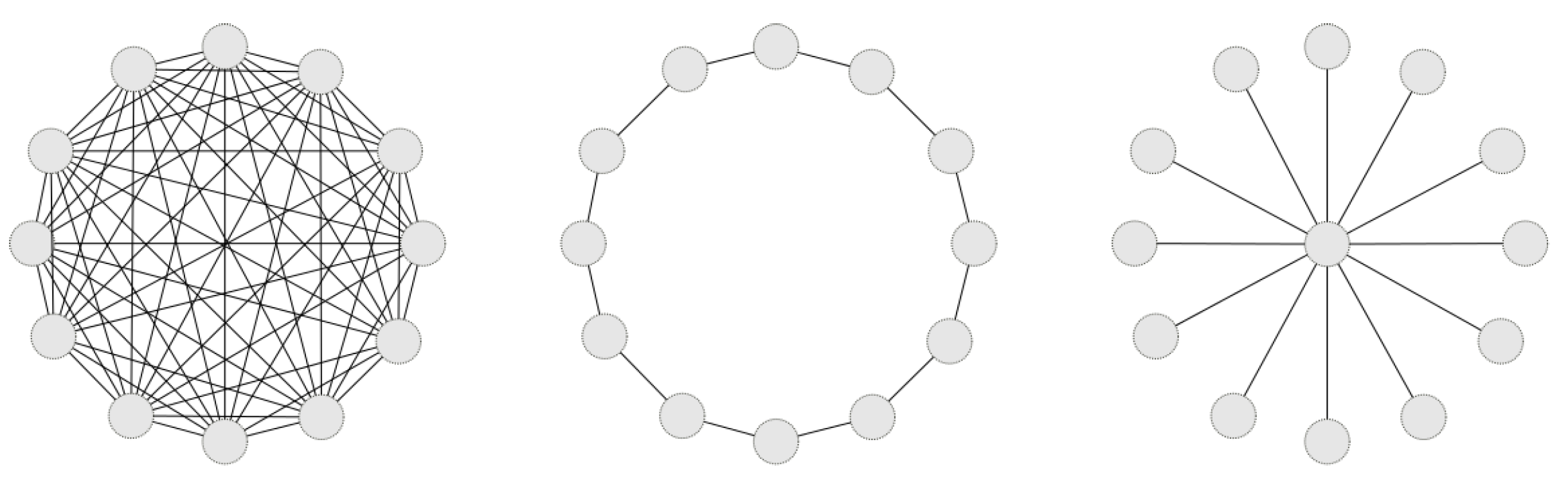
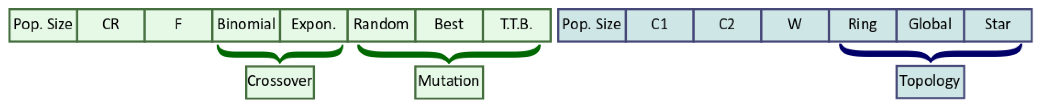
Since the tuner algorithms we consider are real-valued optimization methods, we need a proper representation of the nominal parameters of the LL-EA, i.e., the parameters that encode choices among a limited set of options. We opted for representing each nominal parameter as a real-valued vector with as many elements (genes) as the options available: the actual choice is the one that corresponds to the gene with the largest value. For instance, if the parameter to optimize is PSO topology, we can choose between ring, star and global topology. Each individual in the tuner represents this setting as a three-dimensional vector whose largest element determines the topology used in the LL-EA configuration. These particular genes are mutated and crossed-over following NSGA-II rules just like any other. Figure 3 shows how DE and PSO configurations are encoded.

5. Experimental Evaluation

In this section, we discuss the results of some experiments in which we optimize different performance criteria that can assess the effectiveness of an EA in solving a given optimization task. We take into consideration “classical” criteria pairs, such as solution quality vs. convergence speed, as well as experiments in which the different criteria are represented by different constraints on the available resources (e.g., different fitness evaluation budgets).
To do so, we use DE and PSO as LL-EAs and NSGA-II as EMOPaT’s Tuner-EA. Table 1 shows the ranges within which we let PSO and DE parameters change in our tests. During the execution of the Tuner-EA, all values are actually normalized in the range [ 0 , 1 ] ; a linear scale transformation is then performed whenever a LL-EA is instantiated.
The computation load of the meta-optimization process is heavily dependent on the cost of a single optimization process. If we term t the average time needed for a single run of the LL-EA (which corresponds, for the Tuner-EA, to one fitness evaluation), then the upper bound for the time T needed for the whole process is:
T = t · < Tuner generations > · < Tuner population size > · N
since we can consider the computation time requested by the tuner’s search operators to be negligible with respect to a fitness evaluation. This process can be highly parallelized, since all N repetitions, as well as all evaluations of a population can be run in parallel if enough resources are available. In our tests, we used an 8-core 64-bit Intel(R) CoreTM i7 CPU running at 3.40 GHz; we chose not to parallelize the optimization process but we preferred to parallelize independent runs of the tuners.
EMOPaT has been tested on some functions from the CEC 2013 benchmark [38], with the only difference that the function minima were set to 0.
The code used to perform the tests is available online at http://ibislab.ce.unipr.it/software/emopat.

5.1. Multi-Objective Single-Function Optimization Under Different Constraints

A multi-objective experiment can optimize different functions, the same function under different conditions, etc. Thus, optimizing a single function under different constraints can be seen as a particular case of multi-objective optimization. In this section, we report the results of tests on single-function optimization under different fitness evaluations budgets. Similar experiments can be performed evaluating the function under different conditions (e.g., different problem dimensions) or according to different quality indices as we did in [8] where we considered two objectives (fitness and fitness evaluations budget) for a single function. With respect to that work, the main additional contribution of this section is showing how EMOPaT can be used to generalize the behavior of an EA in optimizing a function when working under different conditions. We consider the following set of quality indices:
{QXi} ≜ best results after {Xi} fitness evaluations, averaged over N runs.
We performed four different tests considering, in each of them, one of the four functions shown in Table 2. Our objectives were the best-fitness values reached after 1000, 10 , 000 and 100 , 000 function evaluations, namely Q1K, Q10K, Q100K. Each test was run 10 times. Doing so, we expected we would favor the emergence of patterns related with the impact of a parameter when looking for “fast-converging” or “slow-converging” configurations. Table 2 summarizes the experimental setup for these experiments.
Firstly, we analyze the LL-EA parameter sets evolved under the different criteria. To do so, we merge the populations of the ten independent runs and, from this pool, we select, for each objective, the top 10 % of the best solutions. For most parameters there is a clear trend as their values monotonically grow or decrease as the fitness evaluations budget increases (see Table 3). This result suggests that, in these cases, it may not be necessary to keep track of all possible computational budgets as in [32], but that the optimal parameters for intermediate objectives may be inferred by interpolating the ones found for the objectives actually taken into consideration; consequently, a developer can use this information to tune its algorithm according to his own budget constraints. Nevertheless, while this can be true for a function, such trends are rarely consistent through different functions, preventing one from drawing more general conclusions.
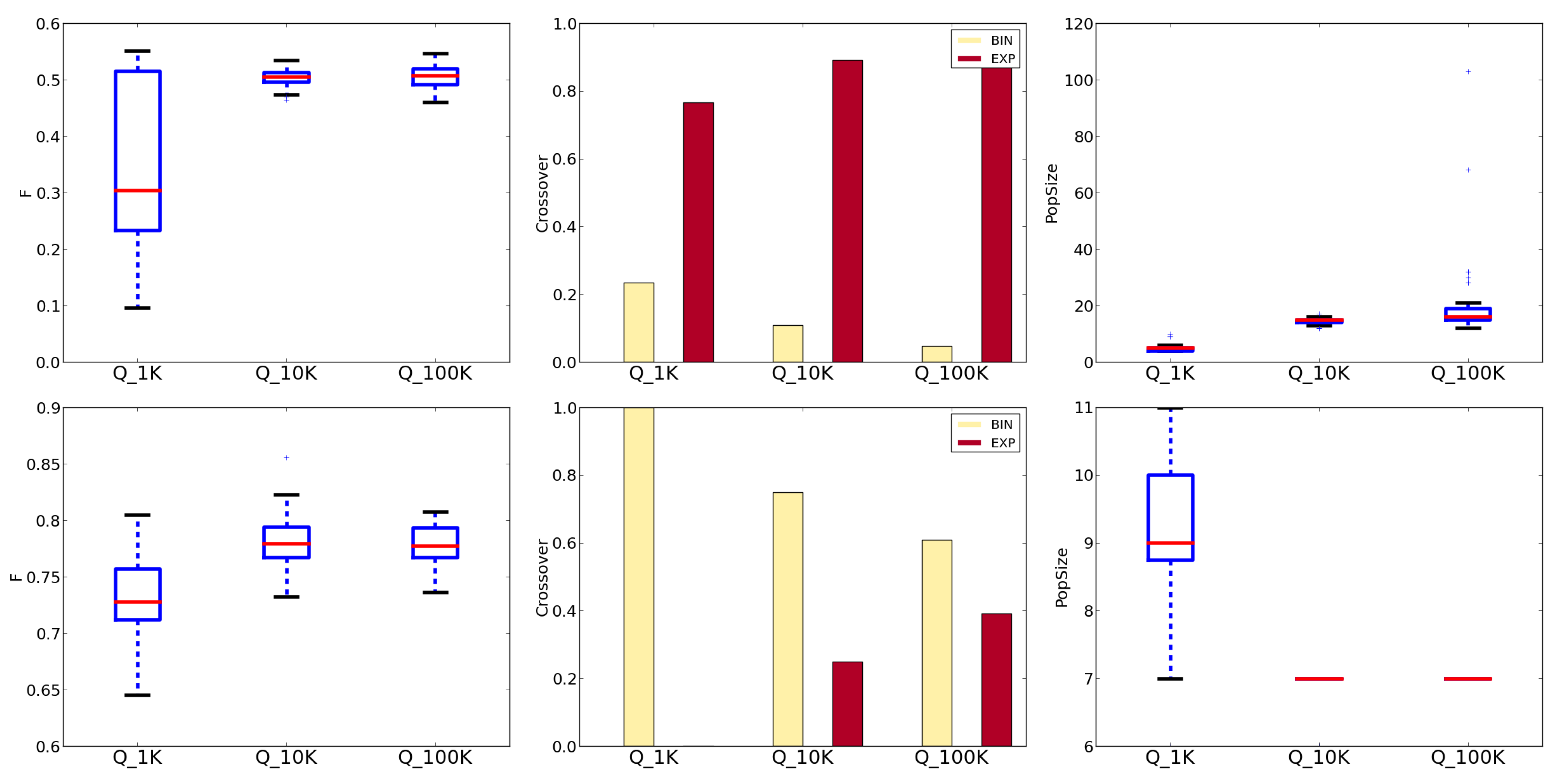
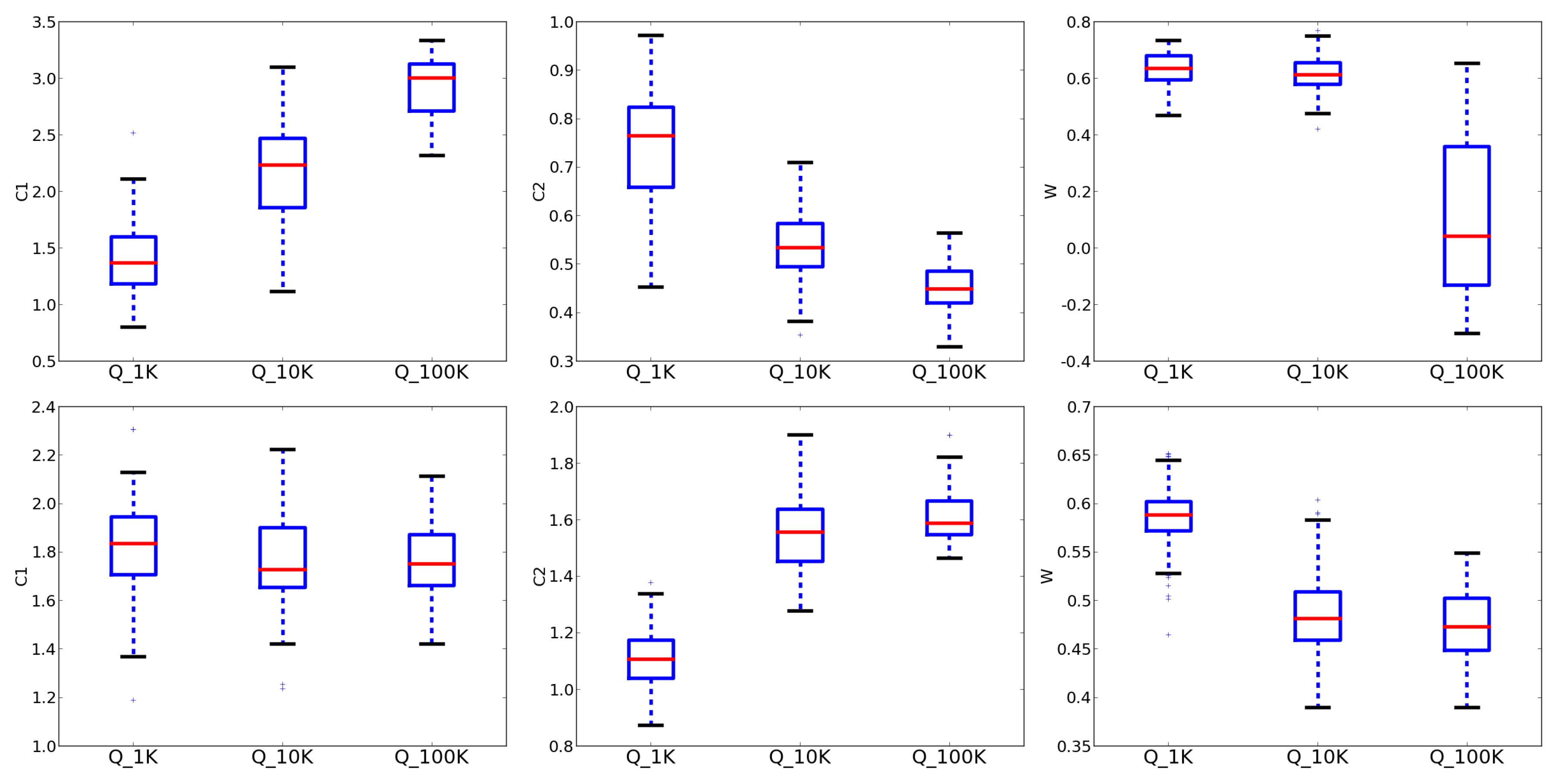
Let us analyze in more details the results on the Rastrigin and the Sphere functions (similar conclusions can be drawn for the other functions). Figure 4 and Figure 5 show the boxplots of some parameters for the top 10 % DE and PSO configurations on these two functions. When parameters are nominal, a bar chart plots the selection frequencies for each option. For the Sphere function, the boxplots of Q10K and Q100K are very similar, pointing out that for this function, 10,000 evaluations are usually sufficient to reach convergence.
To evaluate the hypothesis that intermediate budgets can be inferred from the results obtained on the objectives that have actually been optimized, one can generate new solutions in two ways:
  • infer them as the mean of two top solutions found for two different objectives between which the new objective lies. This approach presents some limitations: (i) the parameter must have a clear trend, (ii) some policy for nominal parameters must be defined if the two reference configurations have different settings, (iii) there is no guarantee that all intermediate values of a parameter correspond to valid configurations of the algorithm;
  • select them from the Pareto front by plotting the set of all the individuals obtained at the end of ten independent runs on the two objectives of interest, estimate the Pareto front based on those solutions and randomly pick one configuration that lies on it, in an intermediate position between the extremes (see an example related with the Rastrigin function in Figure 6).
Table 4 shows the parameters of the best solutions found for the Rastrigin and Sphere functions for the three objectives and of four intermediate solutions generated by the two methods. The ones indicated by A lie between Q1K and Q10K and the ones indicated by B between Q10K and Q100K. It can be noticed that the values of the parameter sets generated using the Pareto Front differ from both the ones inferred as a weighted mean of neighboring ones and the top solutions. In some cases (as with DE on Sphere) these solutions use a mutation type that is never considered by the top solutions. For the nominal parameters of the inferred solutions, we chose to consider both options when the two top solutions disagreed, distinguishing the two solutions by an index (e.g., A 1 and A 2 ).
Figure 7 shows the performance of the configurations considered in Table 4, averaged over 100 independent runs, for DE and PSO. The solid lines represent the Top Solutions; as expected, after 1000 evaluations (see the plots on the right) Q1K is the best-performing configuration, while Q100K is slower in the beginning but is the best at the end of the evolution. In most cases, the inferred solutions have a performance that lies between the performance of the two top solutions used as starting points. The results obtained on the Rastrigin function (first row of Figure 7) are particularly clear: in the first 1000 evaluations, Q1K performs best, then it is surpassed by Inferred A, followed by Q10K, Pareto B, and finally Q100K; this example seems to confirm our general hypothesis. A relevant exception is A 2 in DE Sphere (Figure 7, last row) that performs worse than all others: since its only difference with A 1 is the crossover type, this suggests that it is not possible to infer nominal parameters reliably unless one is clearly prevalent.
Finally, to compare EMOPaT with a state-of-the-art tuner, we implemented the Flexible-Budget method (FBM) proposed by [32]. For a fair comparison, we implemented their method using the same NSGA-II parameters used by EMOPaT, including the budget of LL-EA evaluations. The secondary criterion used to compare equally ranked individuals (see [32] for more details) is the Area Under the Curve. Ten independent runs of FBM were run, after which we selected the solutions that among all runs, had obtained the best-performing configurations after 1 K, 10 K, 100 K evaluations (similar to our setting) and 5.5 K and 55 K evaluations (for a comparison with our inferred parameter sets). Then, we performed 100 runs for each configuration and compared the results to the ones reported in Table 4 (for intermediate values we used the ones called “From Pareto”) allowing the same computational budget. Table 5 shows the parameters found by FBM and Table 6 the comparison between the performance of the two methods. Except for PSO on the Sphere function, for which the results provided by EMOPaT are always better (Wilcoxon signed-rank test, p < 0.01 ), the two tuning methods always obtain equivalent results with budgets of 1 K, 10 K and 100 K evaluations. With the two intermediate budgets, FBM is better three times, EMOPaT is better twice and once they are equivalent; therefore no significant difference between the two methods can be observed.
The results obtained by EMOPaT are also consistent with previous experimental and theoretical findings, such as the ones reported in [39], which proved that premature convergence can be avoided if:
F > 1 C R 2 P o p S i z e
Of the fourteen DE instances in Table 4, Sphere Q1K is the only one that does not respect this condition; this may be an explanation for the fact that this DE version is fast, but generally unable to reach convergence optimizing such a simple unimodal function.

5.2. Multi-Function Optimization

In this section, we show how EMOPaT behaves when the goal is to obtain configurations that perform well on functions that are not included in the “training set”. Following the terminology introduced by [31], we expect to find “generalist” and “specialist” versions of the EAs taken into consideration. Table 7 gives more details about this experiment.
We used EMOPaT to optimize all the seven functions together (repeating the test 10 times) and then we merged all results into a single collection of configurations. From this collection, we selected the best-performing configuration for each of the seven objective functions.
The next step was to select the “generalist” solutions. We consider a “generalist” solution to be a parameter set that does not perform badly on any of the objectives taken into consideration, i.e., it is never in the worst θ percent of the population, when ordered by any objective. Obviously, the higher θ , the lower the number of generalists. We decided to set the value of θ such that seven generalists would be selected, to match the specialists’ number.
Table 8 shows the generalists’ and specialists’ parameters obtained by merging the results of ten independent runs of EMOPaT. An interesting outcome worth highlighting is that, similar to the previous experiment, some of the generalists are not obtained by simply “interpolating” other results but they contain some traits that are not featured by any specialist. For instance, DE G 0 has a smaller population than any specialist, PSO G 3 ’s inertia value is higher than that of all specialists.
A more standard way to infer a “generalist” configuration is to take the one with the best overall results. To do so, we consider the results of all the solutions found by EMOPaT and normalize them so that each fitness has average = 0 and standard deviation = 1; then, we select the configuration that minimizes the sum of the normalized fitnesses. In Table 8, these configurations are reported as “average”.
We also performed 10 meta-optimizations using SEPaT and irace, with the same budget allowed for EMOPaT. The parameters of SEPaT are the ones presented in Table A1, while for irace we used the parameters suggested by the authors. For each optimization method, the ten solutions obtained were compared using the tournament method described in Section 4 to find the best configuration, which is also reported in Table 8.
To test the parameter sets obtained, we selected seven functions from the CEC 2013 benchmark that were not used during training (namely Elliptic, Rotated Discus, Rotated Weierstrass, Griewank, Rotated Katsuura, CF5 and CF7). Table 9 shows, for each function, which configuration(s) obtained the best results. To determine the best function, we performed the Wilcoxon signed-rank test ( p < 0.01 ) on all configurations pairwise. A configuration is considered to be the best if no other configuration performs significantly better on that function. The table shows that, in some cases, generalists were actually able to obtain better results on previously unseen functions than specialists.
Since the definition of “generalist EA” implies the ability not to perform badly on any function, we also analyzed the same data from another viewpoint. Each cell ( i , j ) in Table 10 shows the number of test functions for which the optimizer which row i refers to performs statistically worse than the one referred to by column j (Wilcoxon signed-rank test, p < 0.01 ). The last column reports the sum of each line and can be considered an indicator of the generalization ability of the optimizer with respect to the others over the test functions.
It can be observed that some of the generalists performed very well. The best optimizers for DE were the configurations obtained by SEPaT along with two generalists, G 4 and G 5 . The first two configurations are very similar to each other (same mutation and crossover, C R 0.15 and F 0.5 ), as shown by the presence of statistically significant differences between them only on one function out of seven. No specialist features a similar parameter set. Regarding PSO, two of the specialists ( S c i g a r and S r o s e n b r o c k ) obtained very good results, as well as three of the generalists ( G 0 , G 1 , and G 3 ). It is important to notice that most generalists evolved by EMOPaT outperform the solutions found by the other single-objective tuners used as reference, as well as the one obtained by computing a normalized average of all solutions evolved by EMOPaT (“average” in Table 8). This last configuration (which is the same as S a c k l e y for PSO) was the best optimizer for three functions and the worst one (not reported) for two (Elliptic, Katsuura). This suggests that this is not the correct way of finding a configuration able to perform well on different functions.
In conclusion, we can say that EMOPaT, in a single optimization process, is able to find, at the same time, algorithm configurations that work well on a single function of interest and others that are able to generalize over different unseen functions, while single-objective tuners need separate processes with a consequent increase of the time spent to perform this operation.

6. Summary and Future Work

In this paper we presented some examples of the kind of information and insights into stochastic optimization algorithms that can be offered by a multi-objective meta-optimization environment. To do so, we used EMOPaT, a simple and generic multi-objective evolutionary optimization framework for tuning the parameters of an EA. EMOPaT was tested on the optimization of DE and PSO in different scenarios, showing that it is able to highlight how the parameters affect the performance of an EA in different situations, allowing one to draw generalizable results when considering different constraints applied to the optimization of the same function. Successively, we tested it on different functions and proved it not only allows one to find good configurations for the training function(s), but also to derive from those results new parameter sets that perform well on unseen problems.
We think that EMOPaT can be helpful in many applications and provide useful hints about the behavior of any metaheuristic. In [40] we showed that EMOPaT can be effective in real-world situations, by using it to tune a DE-based object recognition algorithm. In general, a basic application of EMOPaT can be summarized in the following steps, as described also in the code we made available online:
  • Select a proper set of problem-related fitness cases.
  • Select the optimization method(s) whose parameters one wants to tune.
  • Select the objectives to optimize (convergence speed, solution quality, robustness, etc.).
  • Run EMOPaT and save the resulting parameter set.
Below we report some interesting directions towards which this approach can be further expanded:
  • At present, the analysis of the results is essentially a “manual” process. Which is the best way to automatically extract, generalize and infer parameters?
  • EMOPaT belongs to the class of offline parameter tuning algorithms, in which the values of the parameters are set before starting the optimization process and do not change during its execution. Could it also be used to tune the parameters of a population of EA’s online, adapting parameter values as optimization proceeds?
  • In our work, we proved that EMOPaT can also be used to generalize results on a single function (see Section 5.1). Can this idea be extended to different functions? If we obtain a Pareto Front by optimizing two functions, can we extract parameters for a function that lies “between” these two, according to some metric that takes into consideration some of their properties?
  • Is it possible to group or cluster functions based on the best-performing parameters found by EMOPaT?

Author Contributions

Conceptualization, R.U. and S.C.; Investigation, R.U., L.S. and S.C.; Software, R.U.; Supervision, S.C.

Funding

This research received no external funding.

Ethical Approval

This article does not contain any studies with human participants performed by any of the authors.

Conflicts of Interest

The authors declare no conflict of interest.

Appendix A

In this appendix, we first show that EMOPaT can be considered a generalization of its single-objective version SEPaT. This implies that for single-objective optimization problems, we can extend the same conclusions drawn for SEPaT in [5,41] to EMOPaT. Then, to assess its general soundness, we demonstrate EMOPaT’s ability to give insights about the algorithm parameters and on their influence on the optimization process by showing that EMOPaT can correctly deal with some peculiar situations, such as the presence of useless or bad parameters.

Appendix A.1. Comparison with SEPaT

The equivalence between SEPaT and EMOPaT in the single-objective case has been tested on seven functions (see Table A1) from the CEC 2013 benchmark [38], with the only difference that the function minima were set to 0.
First, we performed tuning as a single run of EMOPaT considering these functions as seven different objectives (optimizing all the functions together), and then by running seven times SEPaT, once for each function. More details about these experiments are summarized in Table A1.
Table A1. Comparison between EMOPaT and SEPaT. Experimental settings.
EMOPaT settings *
Tuner EA = NSGA-II, Population Size = 200, 80 Generations,
Mutation Rate = 0.125, Crossover Rate = 0.9
SEPaT settings
Tuner EA = DE, Population Size = 200, 80 Generations
CR = 0.91, F = 0.52, Mutation = target-to-best, Crossover = Exponential
Function settings
10-dimensional Sphere, Rotated Cigar, Rotated Rosenbrock, Rotated Ackley,
Rastrigin, Composition Function 1 (CF1), Composition Function 3 (CF3)
evaluation criterion = best fitness in 20,000 evaluations averaged over N = 15 repetitions.
We checked whether the best solutions for each objective that EMOPaT evolved in a single run (also called “top solutions” or “top configurations” in the following), were actually indistinguishable from those obtained by SEPaT when applied to the same objective. To do so, we ran ten independent experiments with both SEPaT (once for each function) and EMOPaT. The best EA configuration for each function found in each run was then tested 100 times on the optimization of the corresponding function. We computed the median for each set of 100 tests and, based on it, selected the overall best configuration for each function.
Table A2 compares the best PSO and DE configurations obtained by SEPaT in ten independent runs to the best configurations obtained, for each corresponding function, in ten independent runs of EMOPaT; the parameters obtained by the two methods are significantly similar. For instance, the nominal parameters chosen for both DE and PSO are almost always the same except for the PSO topology for Composition Function 3. This is the only case in which the parameters chosen by the two methods are clearly different (one population is three times as large as the other, c 1 is four times larger and the topology is different): nevertheless, the results obtained by the two configurations are virtually equivalent (see Table A3), so the two settings correspond to two equivalent minima of the meta-fitness landscape.
Table A2. Best-performing parameters obtained over 10 runs of EMOPaT and SEPaT, and standard settings for PSO ([42]) and DE ([11]).
Differential Evolution
FunctionMethodPopSizeCRFMutationCrossover
SphereSEPaT200.5060.520target-to-bestexponential
EMOPaT120.1810.718target-to-bestexponential
R. CigarSEPaT600.9550.660target-to-bestbinomial
EMOPaT380.9160.699target-to-bestbinomial
R. RosenbrockSEPaT390.9930.745randomexponential
EMOPaT470.9890.761randomexponential
R. AckleySEPaT850.3270.0randomexponential
EMOPaT2480.9600.0randomexponential
RastriginSEPaT360.0140.359randomexponential
EMOPaT250.0491.065randomexponential
CF 1SEPaT180.01.777bestexponential
EMOPaT330.0451.070bestexponential
CF 3SEPaT890.7940.070randombinomial
EMOPaT980.8680.088randombinomial
-Standard300.90.5randomexponential
Particle Swarm Optimization
FunctionMethodPopSizew c 1 c 2 Topology
SphereSEPaT880.5291.5741.057global
EMOPaT250.7741.9890.591global
R. CigarSEPaT670.7130.5311.130ring
EMOPaT410.7571.1591.097ring
R. RosenbrockSEPaT1040.5971.0321.064ring
EMOPaT87−0.451−0.0921.987ring
R. AckleySEPaT1130.3810.2101.722ring
EMOPaT1150.303−0.0062.467ring
RastriginSEPaT13−0.2360.0903.291global
EMOPaT7−0.2600.0213.314global
CF 1SEPaT92−0.147−0.4622.892ring
EMOPaT61−0.163−0.3763.104ring
CF 3SEPaT610.8520.3470.989ring
EMOPaT2170.7281.2170.565global
-Standard300.7211.1931.193ring
Table A3 shows the median fitness obtained on each function by the best-performing EA configurations found by the tuners and by a standard configuration, and the p-values of Wilcoxon’s signed-rank test under the Null Hypothesis “There are no differences between two configurations’ performance” comparing EMOPaT’s best configuration to SEPaT’s best and to a standard configuration. While, in general, EMOPaT’s configurations perform better than standard parameters (last column), there is no statistical evidence that the best performance of the configurations found by the two methods differ, except for two cases (Rotated Cigar and Rotated Ackley using DE) for which EMOPaT performs slightly better than SEPaT. These results show that EMOPaT can be thought as being generally equivalent to SEPaT in finding the minima of single-objective problems. However, as shown in the paper, one can extract even more information from EMOPaT’s results, thanks to its multi-objective nature.
Table A3. Median fitness over 100 independent runs of the best solutions found by EMOPaT, by SEPaT, and by a standard configuration of the optimization algorithm.
EAFunctionEMOPaTSEPaTStandardvs. SEPaTvs. Standard
Fitnessp-Value
DESphere 0.00 0.00 7.43 E 26 1.00 < 1 E 20
R. Cigar 7.61 E 02 7.64 E 04 1.76 E + 01 4.89 E 03 5.49 E 08
R. Rosenbrock 3.42 E 02 2.76 E 03 9.81 E + 00 0.41 < 1 E 20
R. Ackley 2.04 E + 01 2.05 E + 01 2.05 E + 01 1.21 E 03 9.34 E 07
Rastrigin 0.00 0.00 2.17 E 08 1.00 < 1 E 20
CF 1 2.04 E + 02 2.05 E + 02 4.00 E + 02 0.06 < 1 E 20
CF 3 6.09 E + 02 6.14 E + 02 1.46 E + 03 0.67 < 1 E 20
PSOSphere 0.00 0.00 7.57 E 24 1.00 < 1 E 20
R. Cigar 1.33 E + 06 2.43 E + 06 1.84 E + 06 0.05 0.03
R. Rosenbrock 9.44 E 01 1.01 E + 00 9.81 E + 00 0.87 1.04 E 17
R. Ackley 2.04 E + 01 2.04 E + 01 2.04 E + 01 0.16 0.67
Rastrigin 4.75 E 06 1.02 E 04 1.09 E + 01 0.57 5.88 E 08
CF 1 2.01 E + 02 2.03 E + 02 4.00 E + 02 0.99 < 1 E 20
CF 3 9.62 E + 02 9.85 E + 02 1.16 E + 03 0.27 2.7 E 04

Appendix A.2. Empirical Validation

We have artificially created four test cases characterized by:
  • A useless numerical parameter, i.e., with no effects at all on the algorithm;
  • A harmful numerical parameter, i.e., the higher its value, the worse the fitness;
  • A harmful nominal parameter choice that constantly produces bad fitness values when made;
  • Two totally equivalent choices of a nominal parameter.
A similar approach has been proposed by [43], showing the ability of irace, ParamILS and REVAC to recognize an operator which was detrimental for the fitness. The results of these tests increase the confidence in the actual ability of EMOPaT to recognize the usefulness or, more in general, the role of a parameter of an EA. We limited our tests to optimizing PSO on the Sphere and Rastrigin functions (see Table A4). In these tests, we modified the original encoding of PSO configurations (Figure 3) as shown in Figure A1.
Figure A1. Encoding of PSO configurations in the four cases presented in Appendix A.2. From top left clockwise: useless parameter, harmful numerical parameter, equivalent and harmful topology.
Mathematics 07 00232 g0a1
Table A4. Empirical validation of EMOPaT. Experimental settings.
EMOPaT settings
Population Size = 64, 100 Generations, Mutation Rate = 0.125, Crossover Rate = 0.9
Function settings
30-dimensional Sphere and Rastrigin
evaluation criterion = best fitness in 20000 evaluations averaged over N = 15 repetitions

Appendix A.2.1. Useless Parameter

In this experiment, we extended the PSO configuration encoding by adding a parameter γ that does not appear in the algorithm and therefore has no effects on it. Our goal was to analyze how EMOPaT dealt with such a parameter with respect to the actually effective ones. Table A5 shows mean and standard deviation of the (normalized) numerical parameters in all NSGA-II individuals at the end of ten independent runs. As can be observed, the useless parameter γ has a mean value close to 0.5 and its variance is 0.078 , which is very close to 1 12 , expected for a uniform distribution in [ 0 , 1 ] : this does not happen with the other parameters. Figure A2 plots the values of the Sphere function against the values of PSO parameters (after recovering their actual value). While the values of the real parameters show a clear trend, the values of γ are scattered uniformly all over the graph. As well, the correlation of γ with the other numerical parameters is very low (last row of Table A5). This suggests that a useless parameter can be easily identified by a (quasi-)uniform distribution of its values.
Figure A2. Values of fitness (Sphere function) versus PSO parameters at the end of the tuning procedure. The last graph refers to the useless parameter γ which, unlike the others, spans across all possible values with no correlation with fitness.
Mathematics 07 00232 g0a2
Table A5. Mean and variance values for PSO’s numerical parameters and correlation with a useless one ( γ ). Parameter values are normalized between 0 and 1.
ParameterPopulation Sizew C 1 C 2 γ
Mean0.1590.5550.5860.3320.441
Variance0.03130.01090.01200.01030.0780
Correlation with γ −0.0777−0.179−0.1590.149-

Appendix A.2.2. Harmful Numerical Parameter

In this experiment, we added to the representation of each PSO configuration a parameter β [ 0 , 1 ] whose only effect is to worsen the actual fitness f proportionally to its value as follows:
f ^ = ( f + β ) · ( 1 + β )
Parameter β was constantly assigned values close to 0 (mean 7 × 10 4 , variance 7 × 10 6 ) by EMOPaT. Figure A3 plots values of β versus number of generations, averaged over ten EMOPaT runs. β starts from an average of 0.5 (due to random initialization) but, after a few iterations, its value quickly reaches 0.
Figure A3. Evolution of the “bad parameter” β , averaged over all individuals in ten independent runs of EMOPaT, versus generation number.
Mathematics 07 00232 g0a3

Appendix A.2.3. Harmful Nominal Parameter Setting

In this experiment, we added a “fake” fourth topology to PSO configurations. When it is selected, PSO just returns a bad fitness value. We wanted to verify whether that choice would be always discarded and which values the corresponding gene would take. Figure A4 shows that the fake topology is actually discarded and, after only two generations, is never selected anymore. Moreover, the values of the corresponding gene are always lower than all others; in particular, they are lower than the ones representing the star topology, which is also never selected despite being a valid choice.
Figure A4. Average values and selection percentages of the genes representing the four topologies versus number of EMOPaT generations. Results averaged over 64 individuals in 10 runs.
Mathematics 07 00232 g0a4

Appendix A.2.4. Equivalent Settings

In the last experiment of this section, we added to the basic representation of the PSO configuration a fourth topology that when selected, acts exactly as the global topology. Our goal was to see whether EMOPaT would allow one to understand that the two topologies were in fact the same one. Figure A5 shows the results in the same format as Figure A4. There is no clear correlation between the two “global” versions, but it can be observed that at the end of the evolution, the sum of their selection percentages has converged to the value reached by global in the previous experiment. This means that splitting this choice into two distinct values did not affect EMOPaT’s performance. Nevertheless, these results were reached more slowly, showing that it takes time for EMOPaT to reach the correct values of a nominal parameter when many choices are available.
Figure A5. Average values of the genes representing the four topologies (including the replicated one) and selection percentages. The x axis reports the number of EMOPaT generations.
Mathematics 07 00232 g0a5

References

  1. Eiben, A.E.; Smith, J.E. Introduction to Evolutionary Computing; Springer: Berlin, Germany, 2003. [Google Scholar]
  2. Pitzer, E.; Affenzeller, M. A Comprehensive Survey on Fitness Landscape Analysis. In Recent Advances in Intelligent Engineering Systems; Studies in Computational Intelligence; Fodor, J., Klempous, R., Suárez Araujo, C., Eds.; Springer: Berlin/Heidelberg, Germany, 2012; Volume 378, pp. 161–191. [Google Scholar]
  3. Smith-Miles, K.; Tan, T. Measuring algorithm footprints in instance space. In Proceedings of the IEEE Congress on Evolutionary Computation (CEC), Brisbane, QLD, Australia, 10–15 June 2012; pp. 1–8. [Google Scholar]
  4. Mercer, R.; Sampson, J. Adaptive search using a reproductive metaplan. Kybernetes 1978, 7, 215–228. [Google Scholar] [CrossRef]
  5. Ugolotti, R.; Nashed, Y.S.G.; Mesejo, P.; Cagnoni, S. Algorithm Configuration using GPU-based Metaheuristics. In Proceedings of the Genetic and Evolutionary Computation Conference (GECCO), Amsterdam, The Netherlands, 6–10 July 2013; pp. 221–222. [Google Scholar]
  6. Storn, R.; Price, K. Differential Evolution—A Simple and Efficient Adaptive Scheme for Global Optimization over Continuous Spaces; Technical Report; International Computer Science Institute: Berkeley, CA, USA, 1995. [Google Scholar]
  7. Kennedy, J.; Eberhart, R. Particle Swarm Optimization. In Proceedings of the IEEE International Conference on Neural Networks, Perth, Australia, 27 November–1 December 1995; Volume 4, pp. 1942–1948. [Google Scholar]
  8. Ugolotti, R.; Cagnoni, S. Analysis of Evolutionary Algorithms using Multi-Objective Parameter Tuning. In Proceedings of the Genetic and Evolutionary Computation Conference (GECCO), Vancouver, BC, Canada, 12–16 July 2014; pp. 1343–1350. [Google Scholar]
  9. Deb, K.; Pratap, A.; Agarwal, S.; Meyarivan, T. A fast and elitist multiobjective genetic algorithm: NSGA-II. IEEE Trans. Evolut. Comput. 2002, 6, 182–197. [Google Scholar] [CrossRef] [Green Version]
  10. Deb, K.; Srinivasan, A. Innovization: Innovating design principles through optimization. In Proceedings of the Genetic and Evolutionary Computation Conference (GECCO), Seattle, WA, USA, 8–12 July 2006; pp. 1629–1636. [Google Scholar]
  11. Das, S.; Suganthan, P. Differential Evolution: A Survey of the State-of-the-Art. IEEE Trans. Evolut. Comput. 2011, 15, 4–31. [Google Scholar] [CrossRef]
  12. Montero, E.; Riff, M.C.; Rojas-Morales, N. Tuners review: How crucial are set-up values to find effective parameter values? Eng. Appl. Artif. Intell. 2018, 76, 108–118. [Google Scholar] [CrossRef]
  13. Sipper, M.; Fu, W.; Ahuja, K.; Moore, J.H. Investigating the parameter space of evolutionary algorithms. BioData Min. 2018, 11, 2. [Google Scholar] [CrossRef] [PubMed] [Green Version]
  14. Karafotias, G.; Hoogendoorn, M.; Eiben, Á.E. Parameter control in evolutionary algorithms: Trends and challenges. IEEE Trans. Evolut. Comput. 2015, 19, 167–187. [Google Scholar] [CrossRef]
  15. Nannen, V.; Eiben, A.E. Relevance Estimation and Value Calibration of Evolutionary Algorithm Parameters. In Proceedings of the International Joint Conference on Artifical Intelligence (IJCAI), Hyderabad, India, 6–12 January 2007; pp. 975–980. [Google Scholar]
  16. Larrañaga, P.; Lozano, J.A. Estimation of Distribution Algorithms: A New Tool for Evolutionary Computation; Kluwer Academic Publishers: Norwell, MA, USA, 2001. [Google Scholar]
  17. Smit, S.K.; Eiben, A.E. Beating the ‘world champion’ evolutionary algorithm via REVAC tuning. In Proceedings of the IEEE Congress on Evolutionary Computation (CEC), Barcelona, Spain, 18–23 July 2010; pp. 1–8. [Google Scholar]
  18. Suganthan, P.N.; Hansen, N.; Liang, J.J.; Deb, K.; Chen, Y.P.; Auger, A.; Tiwari, S. Problem Definitions and Evaluation Criteria for the CEC 2005 Special Session on Real-Parameter Optimization; Technical Report, KanGAL Report 2005005; Nanyang Technological University: Singapore, 2005. [Google Scholar]
  19. Meissner, M.; Schmuker, M.; Schneider, G. Optimized Particle Swarm Optimization (OPSO) and its application to artificial neural network training. BMC Bioinform. 2006, 7, 125. [Google Scholar] [CrossRef] [PubMed]
  20. Pedersen, M.E.H. Tuning and Simplifying Heuristical Optimization. Master’s Thesis, University of Southampton, Southampton, NY, USA, 2010. [Google Scholar]
  21. Hutter, F.; Hoos, H.H.; Leyton-Brown, K.; Stützle, T. ParamILS: An Automatic Algorithm Configuration Framework. J. Artif. Intell. Res. 2009, 36, 267–306. [Google Scholar] [CrossRef]
  22. Luke, S.; Talukder, A.K.A. Is the meta-EA a Viable Optimization Method? In Proceedings of the Genetic and Evolutionary Computation Conference (GECCO), Amsterdam, The Netherlands, 6–10 July 2013; pp. 1533–1540. [Google Scholar]
  23. Fister, D.; Fister, I.; Jagrič, T.; Brest, J. A novel self-adaptive differential evolution for feature selection using threshold mechanism. In Proceedings of the 2018 IEEE Symposium Series on Computational Intelligence (SSCI), Bengaluru, India, 18–21 November 2018; pp. 17–24. [Google Scholar]
  24. Bartz-Beielstein, T.; Lasarczyk, C.; Preuss, M. Sequential parameter optimization. In Proceedings of the IEEE Congress on Evolutionary Computation (CEC), Edinburgh, UK, 2–4 September 2005; pp. 773–780. [Google Scholar]
  25. López-Ibáñez, M.; Dubois-Lacoste, J.; Cáceres, L.P.; Birattari, M.; Stützle, T. The irace package: Iterated racing for automatic algorithm configuration. Oper. Res. Perspect. 2016, 3, 43–58. [Google Scholar] [CrossRef] [Green Version]
  26. Pereira, I.; Madureira, A. Racing based approach for Metaheuristics parameter tuning. In Proceedings of the 10th Iberian Conference on Information Systems and Technologies (CISTI), Aveiro, Portugal, 17–20 June 2015; pp. 1–6. [Google Scholar]
  27. Sinha, A.; Malo, P.; Xu, P.; Deb, K. A Bilevel Optimization Approach to Automated Parameter Tuning. In Proceedings of the 2014 Annual Conference on Genetic and Evolutionary Computation (GECCO), Vancouver, BC, Canada, 12–16 July 2014; pp. 847–854. [Google Scholar]
  28. Andersson, M.; Bandaru, S.; Ng, A.; Syberfeldt, A. Parameter Tuning of MOEAs Using a Bilevel Optimization Approach. Evolutionary Multi-Criterion Optimization; Springer: Berlin/Heidelberg, Germany, 2015; pp. 233–247. [Google Scholar]
  29. Dréo, J. Using Performance Fronts for Parameter Setting of Stochastic Metaheuristics. In Proceedings of the Conference on Genetic and Evolutionary Computation Conference (GECCO): Late Breaking Papers, Montreal, QC, Canada, 8–12 July 2009; pp. 2197–2200. [Google Scholar]
  30. Smit, S.K.; Eiben, A.E.; Szlávik, Z. An MOEA-based Method to Tune EA Parameters on Multiple Objective Functions. In Proceedings of the International Conference on Evolutionary Computation, (part of the International Joint Conference on Computational Intelligence IJCCI (ICEC)), Valencia, Spain, 24–26 October 2010; pp. 261–268. [Google Scholar]
  31. Smit, S.K.; Eiben, A.E. Parameter Tuning of Evolutionary Algorithms: Generalist vs. Specialist. In Applications of Evolutionary Computation; Di Chio, C., Brabazon, A., Ebner, M., Farooq, M., Fink, A., Grahl, J., Greenfield, G., Machado, P., O’Neill, M., Tarantino, E., et al., Eds.; LNCS Springer: Berlin/Heidelberg, Germany, 2010; Volume 6024, pp. 542–551. [Google Scholar]
  32. Branke, J.; Elomari, J.A. Meta-optimization for Parameter Tuning with a Flexible Computing Budget. In Proceedings of the Conference on Genetic and Evolutionary Computation Conference (GECCO), Philadelphia, PA, USA, 7–11 July 2012; pp. 1245–1252. [Google Scholar]
  33. Eiben, A.E.; Smit, S.K. Parameter tuning for configuring and analyzing evolutionary algorithms. Swarm Evol. Comput. 2011, 1, 19–31. [Google Scholar] [CrossRef] [Green Version]
  34. Blot, A.; Hoos, H.H.; Jourdan, L.; Kessaci-Marmion, M.É.; Trautmann, H. MO-ParamILS: A multi-objective automatic algorithm configuration framework. In Proceedings of the International Conference on Learning and Intelligent Optimization, Ischia, Italy, 29 May–1 June 2016; pp. 32–47. [Google Scholar]
  35. Blot, A.; Pernet, A.; Jourdan, L.; Kessaci-Marmion, M.É.; Hoos, H.H. Automatically configuring multi-objective local search using multi-objective optimisation. In Evolutionary Multi-Criterion Optimization; Springer: Cham, Switzerland, 2017; pp. 61–76. [Google Scholar]
  36. López-Ibánez, M.; Dubois-Lacoste, J.; Stützle, T.; Birattari, M. The Irace Iackage, Iiterated Iace for Automatic Algorithm Configuration; Technical Report TR/IRIDIA/2011-004; IRIDIA, Université Libre de Bruxelles: Bruxelles, Belgium, 2011. [Google Scholar]
  37. Smit, S.K.; Eiben, A.E. Comparing Parameter Tuning Methods for Evolutionary Algorithms. In Proceedings of the IEEE Congress on Evolutionary Computation (CEC), Trondheim, Norway, 18–21 May 2009; pp. 399–406. [Google Scholar]
  38. Liang, J.; Qu, B.; Suganthan, P. Problem Definitions and Evaluation Criteria for the CEC 2013 Special Session on Real-Parameter Optimization; Technical Report; Computational Intelligence Laboratory, Zhengzhou University: Zhengzhou, China; Nanyang Technological University: Singapore, 2013. [Google Scholar]
  39. Zaharie, D. Critical values for the control parameters of Differential Evolution algorithms. In Proceedings of the 8th International Conference on Soft Computing, Brno, Czech Republic, 5–7 June 2002; pp. 62–67. [Google Scholar]
  40. Ugolotti, R.; Cagnoni, S. Multi-objective Parameter Tuning for PSO-based Point Cloud Localization. In Advances in Artificial Life and Evolutionary Computation. Proceedings of WIVACE 2014, Vietri sul Mare, Italy, 14–15 May 2014; Pizzuti, C., Spezzano, G., Eds.; Communications in Computer and Information Science; Springer: Berlin/Heidelberg, Germany, 2014; Volume 445, pp. 75–85. [Google Scholar]
  41. Ugolotti, R.; Mesejo, P.; Nashed, Y.S.G.; Cagnoni, S. GPU-Based Automatic Configuration of Differential Evolution: A Case Study. In Progress in Artificial Intelligence; Springer: Berlin/Heidelberg, Germany, 2013; pp. 114–125. [Google Scholar]
  42. Kennedy, J.; Clerc, M. 2006. Available online: http://www.particleswarm.info/Standard_PSO_2006.c (accessed on 2 March 2019).
  43. Montero, E.; Riff, M.C.; Pérez-Caceres, L.; Coello Coello, C. Are State-of-the-Art Fine-Tuning Algorithms Able to Detect a Dummy Parameter? In Parallel Problem Solving from Nature Conference—PPSN XII, LNCS, Proceedings of the 12th International Conference, Taormina, Italy, 1–5 September 2012; Coello, C.A., Cutello, V., Deb, K., Forrest, S., Nicosia, G., Pavone, M., Eds.; Springer: Berlin/Heidelberg, Germany, 2012; Volume 7491, pp. 306–315. [Google Scholar]
Figure 1. The three PSO topologies used in this work: global, ring, and star.
Mathematics 07 00232 g001
Figure 2. Scheme of SEPaT/EMOPaT. The lower part represents a classical EA. In the meta-optimization process, each individual of Tuner-EA represents a set of Parameters. For each set, the corresponding instance of the lower-level EA (LL-EA) is run N times to optimize the objective function(s). Quality indices (one for SEPaT, more than one for EMOPaT) are values that provide a global evaluation of the results obtained by LL-EA in these runs.
Mathematics 07 00232 g002
Figure 3. Encoding of DE (left) and PSO (right) configurations in a tuner EA.
Mathematics 07 00232 g003
Figure 4. DE parameters of the top solutions (best 10 % ) for the 30-dimensional Rastrigin (first row) and Sphere (second row) functions, with an available budget of 1000, 10,000, and 100,000 fitness evaluations. Bar plots indicate the normalized selection frequency. Descending/ascending trends for all parameter values are clearly visible.
Mathematics 07 00232 g004
Figure 5. PSO parameters of the top solutions (best 10 % of the population) for the 30-dimensional Rastrigin (first row) and Sphere (second row) functions, with an available budget of 1000, 10,000, and 100,000 fitness evaluations. Descending/ascending trends for all parameter values are clearly visible.
Mathematics 07 00232 g005
Figure 6. Fitness values of all the solutions found in ten independent runs of EMOPaT for the three criteria, plotted pairwise for adjacent values of the budget. The green and red stars represent the Top Solutions for each objective, yellow circles are candidate solutions for intermediate evaluation budgets.
Mathematics 07 00232 g006
Figure 7. Average fitness versus number of fitness evaluations for configurations generated for PSO (first and second rows) and DE (third and fourth) for the 30-dimensional Rastrigin (above) and Sphere (below) functions. The plots on the right magnify the first 1000 evaluations to better compare the performance of the “fast” versions.
Mathematics 07 00232 g007
Table 1. Search ranges for the DE and PSO parameters. We chose ranges that are wider than those usually considered in the literature, to allow SEPaT and EMOPaT to “think outside the box”, and possibly find unusual parameter sets.
Differential EvolutionParticle Swarm Optimization
Population Size [ 4 , 300 ] Population Size [ 4 , 300 ]
Crossover Rate (CR) [ 0.0 , 1.0 ] Inertia Factor (w) [ 0.5 , 1.5 ]
Scale Factor (F) [ 0.0 , 2.0 ] c 2 [ 0.5 , 4.0 ]
Crossover{binomial, exponential} c 1 [ 0.5 , 4.0 ]
Mutation{random, best, target-to-best}Topology{ring, star, global}
Table 2. Single-function optimization with different fitness evaluation budgets. Experimental settings.
EMOPaT settings
Population Size = 64, 60 Generations, Mutation Rate = 0.125, Crossover Rate = 0.9
Function settings
30-dimensional Sphere, Rastrigin, Rosenbrock, Griewank (one for each experiment)
evaluation criterion = best fitnesses after 1000, 10,000, 100,000 evaluations averaged
over N = 15 repetitions.
Table 3. Trends of DE and PSO parameter values versus fitness evaluations budget. Upward arrows denote parameter values increasing with the number of evaluations, downward arrows the opposite. A dash denotes no clear trend. For nominal parameters, the table reports the most frequently selected choice. If the choice changes within the top solutions for different evaluation budgets, an arrow shows the direction of this change as the budget increases.
Differential Evolution
FunctionPopSizeCRFMutationCrossover
Spheretarget-to-bestbinomialexponential
Rastriginbinomialexponential
Griewanktarget-to-bestrandombinomial
Rosenbrocktarget-to-bestbest,randombinomialexponential
Particle Swarm Optimization
FunctionPopSizew c 1 c 2 Topology
Spherering
Rastriginglobal
Griewankring
Rosenbrockglobalring
Table 4. DE and PSO configurations for the same objective function with three different fitness evaluations budgets.“Top Solutions” are the best-performing sets on each objective; “Inferred” refers to the ones obtained averaging Top Solutions; “From Pareto” are extracted from the Pareto front obtained considering the objectives pairwise (see Figure 6).
Differential Evolution
MethodConfigurationPopSizeCRFMutationCrossover
RastriginTop SolutionsQ1K90.2140.736target-to-bestbinomial
Q10K70.0530.754target-to-bestexponential
Q100K70.0390.784target-to-bestexponential
Inferred A 1 , A 2 80.1340.745target-to-bestbin., exp.
B70.0460.769target-to-bestexponential
From ParetoA90.2170.763target-to-bestbinomial
B70.0060.769target-to-bestbinomial
SphereTop SolutionsQ1K50.0220.229randombinomial
Q10K140.3630.508randomexponential
Q100K300.0430.521randomexponential
Inferred A 1 , A 2 90.1920.368randombin., exp.
B220.2030.514randomexponential
From ParetoA80.0230.520target-to-bestexponential
B15 0.50 E 3 0.498target-to-bestbinomial
Particle Swarm Optimization
MethodConfigurationPopSizew c 1 c 2 Topology
RastriginTop SolutionsQ1K180.5601.1950.789global
Q10K260.5792.4920.671global
Q100K76 0.251 2.5330.487global
InferredA220.5691.8440.730global
B510.1642.5130.579global
From ParetoA270.6780.9490.587global
B600.2973.1320.481global
SphereTop SolutionsQ1K110.6031.8821.105ring
Q10K140.5101.9981.483ring
Q100K150.4491.7251.667ring
InferredA120.5571.9401.294ring
B150.4801.8611.575ring
From ParetoA140.6491.7641.082ring
B150.4801.6811.635ring
Table 5. DE and PSO configurations obtained by the Flexible-Budget Method [32].
Differential Evolution
BudgetPopSizeCRFMutationCrossover
Rastrigin1 K50.3750.375randomexponential
5.5 K90.1820.182randomexponential
10 K160.1450.145randomexponential
55 K240.1460.146randomexponential
100 K750.7460.746randomexponential
Sphere1 K160.2990.554target-to-bestbinomial
5.5 K70.0690.751target-to-bestexponential
10 K70.0560.749target-to-bestexponential
55 K70.0570.749target-to-bestexponential
100 K70.0570.749target-to-bestexponential
Particle Swarm Optimization
BudgetPopSizew c 1 c 2 Topology
Rastrigin1 K110.6641.5180.638global
5.5 K880.6621.0620.624global
10 K1190.6541.6720.607global
55 K2300.6502.4120.643global
100 K2300.6502.4120.643global
Sphere1 K170.8370.9520.488global
5.5 K320.8970.5390.545global
10 K320.8970.5390.545global
55 K340.3801.1352.673global
100 K340.3801.1352.673global
Table 6. Comparison between the performance of the configurations found by EMOPaT and the Flexible-Budget method (FBM).
Differential Evolution
BudgetEMOPaTFBMp-ValueBest Method
Rastrigin1 K 7.68 E + 01 7.76 E + 01 1.42 E 01
5.5 K 4.29 E + 00 5.06 E + 00 8.53 E 03 EMOPaT
10 K 3.32 E 02 1.04 E 01 4.49 E 01
55 K 5.68 E 14 0.00 E + 00 1.43 E 08 FBM
100 K 0.0 0.0 8.33 E 02
Sphere1 K 1.11 E + 02 1.08 E + 02 9.62 E 03 EMOPaT
5.5 K 6.51 E + 01 5.32 E + 01 3.62 E 11 FBM
10 K 4.24 E + 01 4.15 E + 01 6.52 E 01
55 K 2.45 E + 01 2.53 E + 01 1.28 E 01
100 K 0.0 0.0 2.49 E 01
Particle Swarm Optimization
BudgetEMOPaTFBMp-ValueBest Method
Rastrigin1 K 8.77 E + 02 1.04 E + 03 9.51 E 01
5.5 K 5.10 E 04 5.19 E 05 3.23 E 05 FBM
10 K 6.13 E 13 5.69 E 13 4.98 E 01
55 K 2.64 E 93 4.27 E 93 5.58 E 03 EMOPaT
100 K 1.79 E + 01 2.03 E + 01 7.05 E 02
Sphere1 K 7.16 E + 02 1.40 E + 03 1.33 E 13 EMOPaT
5.5 K 1.03 E 02 8.18 E + 00 3.90 E 18 EMOPaT
10 K 1.96 E 07 1.11 E 01 3.90 E 18 EMOPaT
55 K 1.46 E 56 2.23 E 22 3.86 E 18 EMOPaT
100 K 0.0 5.15 E 44 3.88 E 18 EMOPaT
Table 7. Optimization of seven different functions. Experimental settings.
EMOPaT settings
Population Size = 200, 80 Generations, Mutation Rate = 0.125, Crossover Rate = 0.9
Function settings
10-dimensional Sphere, Rotated Cigar, Rosenbrock, Rotated Ackley,
Rastrigin, Composition Function 1 (CF1), Composition Function 3 (CF3)
evaluation criterion = best fitness in 20000 evaluations averaged over N = 15 repetitions.
Table 8. The seven DE and PSO best-performing configurations generated by EMOPaT for each “training” function (denoted by S, for specialist, followed by the name of the function); the seven configurations that never achieved bad results in any of them (denoted by G, for generalist); the parameter sets found by irace and by SEPaT; and the single generalist configuration obtained by normalizing fitness values (see text).
Differential Evolution
Configuration NamePopSizeCRFMutationCrossover
S s p h e r e 120.1810.718target-to-bestexponential
S c i g a r 570.9060.703target-to-bestexponential
S r o s e n b r o c k 470.9890.761randomexponential
S a c k l e y 2710.1700.216target-to-bestexponential
S r a s t r i g i n 240.0241.158randomexponential
S C F 1 240.0571.789bestexponential
S C F 3 980.8680.087randombinomial
G 0 100.6070.886target-to-bestexponential
G 1 700.6120.480bestexponential
G 2 130.2350.444target-to-bestexponential
G 3 230.4130.860target-to-bestexponential
G 4 320.1470.491target-to-bestexponential
G 5 240.7760.716target-to-bestexponential
G 6 190.0580.837bestbinomial
irace530.7960.508bestexponential
SEPaT170.1600.499target-to-bestexponential
average400.5630.988target-to-bestbinomial
Particle Swarm Optimization
Configuration NamePopSizew c 1 c 2 Topology
S s p h e r e 340.7681.7560.474global
S c i g a r 410.5851.3381.646ring
S r o s e n b r o c k 55−0.465−0.0601.930ring
S a c k l e y 2510.7141.0820.271global
S r a s t r i g i n 20−0.131−0.0503.787global
S C F 1 161−0.158−0.1122.467ring
S C F 3 269−0.1721.2351.945global
G 0 430.6481.2411.633ring
G 1 440.6392.1141.478ring
G 2 680.4021.1092.184ring
G 3 370.8830.5480.649ring
G 4 26−0.0730.2953.032ring
G 5 330.5832.0401.677ring
G 6 460.5931.9441.637ring
irace190.8050.9620.914ring
SEPaT220.7321.3581.153ring
average2510.7141.0820.271global
Table 9. Best-performing DE and PSO configurations on the seven test functions.
FunctionDEPSO
Elliptic S s p h e r e irace, SEPaT
Discus S c i g a r average, S a c k l e y
Weierstrass S c i g a r , irace S s p h e r e , S r o s e n b r o c k
Griewank S r a s t r i g i n , SEPaT, G 4 G 0 , G 1 , G 2 , G 5 , G 6 , S c i g a r
Katsuura G 2 , SEPaT, G 4 S C F 1 , S r o s e n b r o c k
CF5 S c i g a r , SEPaT S a c k l e y , average
CF7 G 2 , SEPaT, G 4 S a c k l e y , S r o s e n b r o c k , average
Table 10. Number of test functions for which the optimizer associated with the row is statistically worse than the one associated with the column. The last column reports the sum of the values in that row, measuring the optimizer performance (the lower, the better). The three best configurations are highlighted in bold.
S sphere S cigar S rosenbrock S ackley S rastrigin S CF 1 S CF 3 G 0 G 1 G 2 G 3 G 4 G 5 G 6 iraceSEPaTaveragesum
Differential Evolution
S s p h e r e 0444304445364246259
S c i g a r 2001111314232224130
S r o s e n b r o c k 3602422344345344255
S a c k l e y 3440322445354345459
S r a s t r i g i n 1322002335363335145
S C F 1 4534704477577567385
S C F 3 2533320434343344252
G 0 2441203043146254247
G 1 2420102104244234237
G 2 2321103230034132131
G 3 2432204343065146352
G 4 1331002311103131125
G 5 1310101003130123020
G 6 1442204242054044244
irace1311210123133103127
SEPaT1221002210013130120
average2533314344365255058
Particle Swarm Optimization
S s p h e r e 0343221333323323343
S c i g a r 4044043020101211431
S r o s e n b r o c k 1202002222312222227
S a c k l e y 3330322333333333043
S r a s t r i g i n 5674045666656666488
S C F 1 2235103222222222539
S C F 3 4344220322333333448
G 0 4144032020101211430
G 1 1234131201321121331
G 2 4144043110212211435
G 3 2234032211012211431
G 4 4444054433404344458
G 5 3434142112310133440
G 6 2234131201221022432
irace4244143233323301446
SEPaT4244143222212300440
average3330322333333333043

