Effects of Preservation Technology Investment on Waste Generation in a Two-Echelon Supply Chain Model

Abstract

This study develops an integrated production-inventory model for a two-echelon supply chain network with controllable probabilistic deterioration. The investment in preservation technology is considered a decision variable to control the deteriorated quantity of an integrated system. The objective of the study is to optimize preservation investment, the number of shipments and shipment quantity, so that the total cost per unit of time of the supply chain is minimized. The study proposes a solution method, and the results show that investment in preservation technology reduces the total supply chain cost by 13%. Additionally, preservation increases the lot size, thus increasing the production cycle length, which reduces the ordering cost of the system. Furthermore, this study shows that preservation leads to a reduction of solid waste from deteriorated products. Total deteriorated products reduced to 8 units from 235 units, hence, preservation generates positive environmental benefits along with economic impacts. The robustness of the proposed model is illustrated with a numerical example, sensitivity analysis, and graphical representations. Moreover, comparative study and managerial insights are given to extract significant insights from the model.

1. Introduction

The phenomena of deterioration are referred to as spoilage, damage, vaporization or other changes in product quality or productivity because of environmental changes during storage. Products like semiconductor chips, battery, volatile liquids, seafood, and medicinal items like blood, deteriorate with time and lose their usefulness over their lifetime. In the existing literature, the deterioration is considered either a constant or random aspect of products. In reality, deterioration of products is a controllable factor which can be modified through investment in adequate preservation technology. Preservative technology contributes to the increased lifespan of materials by maximizing how efficiently they are processed. Similarly, preservation aids in lowering the amount of contamination generated in a commodity-to-product conversion or storage setup, and it also reduces the required number of material supplies too. For instance, the decay of the cement matrix under certain environmental factors is decreased using pozzolanic additives, which also reduces the calcium-leeching effect of cement substance in the environment [1]. Carbon emissions also reduce up to 12%, and energy efficiency is enhanced by utilizing 19% less natural reserves with this additive.

In multi-echelon supply chain structures, the impacts of deterioration are increased compared to the single player structure. Because the same product faces deterioration multiple times at every stage. A supply chain infrastructure usually comprises processing units and retail units. A product goes through several processes in a supply chain infrastructure; from supply to the conversion of raw materials, and, to the storage of finished products. The capacity of each unit to adjust production quantity and assure the adequately long shelf life is another important aspect of supply chain coordination. For instance, fruit or chemical processing units invest in decay preventive packaging or additives for their products. Then a retail unit must be equipped with appropriate preservation equipment (required environmental and temperature conditions) for reception and storage of such products. However, in the existing literature, simultaneous preservation efforts in multi-echelon supply chain management have been overlooked. Preservation investment is considered to be the personal preference of the individual players of the supply chain. However, in reality, multiple members of the supply chain can invest in their setups simultaneously to enhance the credibility and efficiency of preservation technology. There is a need to encourage production firms and retailers to organize, diversify and upgrade their commodities-inventory and business setup. Investments in infrastructure, production techniques, storage, packaging, and transportation are also required to reduce product deterioration and enhance supply chain system efficiency.

The deteriorated items waste is mainly associated with managerial and technical limitations in firms. Moreover, it is also related to a lack of coordination between the different players of a supply chain. As the supply chain is a dynamic system, the products are needed to be capable of readapting several processing environments as they face frequent changes from processing units to retail units. The lack of coordination between the supply chain increases the impact of deterioration from one stage to another. Consequently, waste due to the deterioration of products is generated in every stage of the supply chain. Inescapably, this also means that a large number of resources are drained away in the supply chain with no purpose fulfilled. Also, waste disposal costs of deteriorated items have not been considered in existing deteriorated inventory studies, where, practically supply chain members bear extra cost to deposit waste safely. The coordination of certain aspects, like costs and quality of products in a supply chain infrastructure, is a fundamental parameter in keeping product cost in-control and making a supply chain profitable. To overcome these limitations, this study highlights the waste conception due to deterioration in the supply chain system. Further, it develops an assessment study of the waste quantity management, and, provides a waste control strategy in terms of preservation investment.

The rest of the paper is organized as follows: A comprehensive literature review is provided in Section 2. Problem definition, notation and assumptions for the proposed model are presented in Section 3. The mathematical model formulation is addressed in Section 4. Numerical examples, the comparison between models with and without preservation investment and sensitivity analysis are provided in Section 5. Finally, the conclusion and future research are given in Section 6.

2. Literature Review

In this section, we thoroughly overview the related research areas of this paper. Three research areas are examined in this study, namely: controllable probabilistic deterioration rate; waste generation from deteriorated items; and preservation investment.

2.1. Controllable Probablistic Deterioration Rate

The consideration of deterioration has got significant attention in inventory-based research with constant deterioration rates, supply chain coordination and price discounts. For the first time, Ghare [2] analyzed the effect of the constant rate of decay on a classical EOQ model under constant demand and no shortages. However, practically, the life expectancy and failure rate of products are better observed with the variable deterioration rate. Covert and Philip [3] extended the case of product deterioration rate to a variable phenomenon. They consider a two-parameter Weibull distribution. Sarkar et al. [4] examines the time-varying deterioration rate for fixed lifetime products. They have also considered full trade and partial trade credit policy for deteriorated inventory. Philip [5], Mukhopadhyay et al. [6], and Hung [7] examined optimal inventory policy with the product loss because of deterioration, treating the deterioration rate as a time-varying function. Sarkar et al. [8] proposed an optimal cycle length model with time-varying deterioration and a partial backlogging rate. Shah et al. [9] discussed a time-varying deteriorated inventory system and introduced temporary price discounts for decayed products. Tadikamalla [10] studied the Gamma distribution based on the distribution pattern for the deterioration rate. Several authors examine the decay of products in terms of entropy [11,12]. The work relates entropy with the product’s geometrical aspect and their intended physical performance. Sarkar [13] discuss a time-dependent demand and deterioration rate model. In this study, a trade-credit is offered to retailers by suppliers to buy extra deteriorated items with different discount rates. Ahmad et al. [14] reviewed the product deterioration and damage during transportation. Decaying inventory models for agricultural products were studied by Ning et al. [15], and the demand rate of products is considered as a function of product price and freshness. They examined a decrease in profit with increased cycle time for decaying products. Guariglia [16] examined the geometric configuration of products. The study discusses the performance of products based on their entropy characteristics.

Sarkar [17] examined the deteriorated inventory model with random rates of decay. The study examines different distributions for deterioration rates such as uniform, triangular and beta distributions. Iqbal and Sarkar [18] proposes a production model for an integrated imperfect and deteriorating production system. The study associates the total system cost with minimization regarding the production rate and cycle time. A deteriorating inventory model for the two-warehouse system was examined by Sett et al. [19]. The proposed model considers time-dependent deterioration for products with a quadratic demand function. An optimal replenishment policy model for deteriorating was developed by Sett et al. [20]. An economic manufacturing quantity model with deteriorating items and system unreliability under inflation and time value of money was studied by Sarkar and Sarkar [21]. They developed a reliable production system with investment in technology development to improve the reliability parameter. The study considers ramp-type demand for perishable products with a fixed life and deterioration as a linear function of time. A detailed review on deteriorating inventory models was provided by Bakker et al. [22]. The existing literature considers the phenomena of deterioration as a constant or variable parameter, whereas it is more realistic to recognize it as a controllable factor with making additional capital investments. To address the practical aspects of decay in the supply chain, we consider the controllable probabilistic deterioration of products in an integrated-inventory problem.

2.2. Waste Generation from Deteriorated Items

Product management after its life cycle has got much attention in literature. The need for repairable/recycled strategies for the used product inventory problem was acknowledged back in 1960. The recovered/repaired products could account for up to 50% of the original investment in inventory [23]. However, product waste generation due to deterioration before its use has not got much attention from researchers. Solid waste generation and resource wastage is predestined with deteriorating products. Some product’s losses begin on production units even before reaching retail like foods, fruits and liquids. Deterioration cause changes in the quality, availability and wholesomeness of products that prevent them from being consumed and they end up as discarded material on both the manufacturer’s and retailer’s end. Deteriorated item’s waste are actually well produced goods intended for consumption which are subsequently degraded or contaminated. These discarded deteriorated products have an adverse impact on the economic, social and environmental level. A multi-stage production system under uncertainties and process imperfection was studied in Tayyab et al. [24]. From an environmental point of view, disposing of deteriorated products contributes to additional greenhouse gas (GHG) emissions. It also leads to increased resource depletion and material wastage [25]. Financial impacts of deterioration on a firm are because of extra costs related to resource wastage and lost sales. Whereas, system quality of the firm refers to improved productivity and less wastage generation, where both rely on reduced system deterioration and maximized resource utilization.

The causes of decay in production systems are mainly associated with financial, technical and managerial limitations. These limitations affect production, storage, packaging techniques, transportation, and marketing systems. There is a need to improve factors which influence system resources to improve system productivity. The drivers for waste generation related to production, deterioration and handling were discussed by Thyberg and Tonjes [26]. Tayyab et al. [27] examined the manufacturing process to optimize a sustainable lot size to achieve simultaneous economic and environmental viability. The study also provides insights into waste prevention policies for a sustainable supply chain with deteriorating inventories. The pull approach and recycling concept is also considered in the literature to avoid potential waste from decayed and damaged products. Decay in raw material inventory, work-in-process inventory, and finished goods with proper disposal was discussed by Tibben-Lembke [28]. The efficient management of assets is considered a key parameter in overcoming the negative impacts of unsolicited costs on firm finances. Deterioration creates a waste of products in every supply chain, and this waste is generally considered a replaceable but not reusable commodity for a firm. For example, once deteriorated, then oils, resins, spare-part lubricators, chemicals, food, cosmetics, medicine, and biological matters are identified as non-reusable products. Inevitably, this also indicates that a large number of supplies are wasted away in the supply chain with no purpose fulfilled. Additionally, the deterioration increases the required quantity of raw material by contaminating non-deteriorated raw material inventory. In reality, supply chain members bear extra costs to deposit waste created from product deterioration. Hence, we introduced the waste disposal costs of deteriorated items to make this study more practical.

2.3. Preservation Tecniques

Economically, the deterioration of products has a direct and negative impact on the finances and brand image of a firm. High deterioration rates are entitled with higher annual costs, shortages and lost sales. On this account, business organizations are interested in comprehending the causes of deterioration and developing approaches to preserve their produced goods and increase profit. There is economic and environmental consciousness that pressurizes manufacturers to extend the useable lives of their products and reduce waste to conserve natural resources. Therefore, there is a need to initiate such product recovery systems in manufacturing units as well as at retail ends that reduce deterioration and wastage of resources. Practically, the deterioration rate of goods can be controlled and reduced through procedural/environmental changes and advanced equipment acquisition. These procedural changes entitled as preservation investment are meant to prevent, delay, or eventually reduce the deterioration/decay of goods. Many business entities invest in advanced equipment to extend product expiration dates. Murr and Morris [29] showed that a low storage temperature leads to a decrease in decay and increases the storage life of products. Investment in vacuum technology leads to a reduction in the deterioration rate of food and medicinal items. SO₂ fumigation was used to develop a color retention technique for fruits by Zauberman et al. [30]. Yang et al. [31] and Ho et al. [32] states that improved storage conditions reduce the total relevant inventory costs for deteriorating products. Waste management in the uncertain environment was examined by Habib et al. [33].

Nye et al. [34] investigates the effect of production batch size and investments in setup cost reduction. Lee [35] developed an economic assessment model for investment strategies in an imperfect production system and considered a preventive maintenance strategy to decrease system deterioration. Lin and Hou [36] examined an inventory system with random yields. This study considers added capital investment in the system to reduce yield variability and setup cost. An investment in supplier’s management cost was added to reduce lead time by Hsu and Wee [37]. This study develops a deteriorating inventory replenishment model with an expiration date and uncertain lead time. Li et al. [38] developed a return-on-investment maximization model; the study examined the effect of the capital investment on setup and quality operations under budget constraints. The potential impact of investments in setup cost reduction and quality improvement was examined by Affisco et al. [39]. The study suggests that decreasing deterioration is not a linear function of investment. Uçkun et al. [40] developed an optimal investments level model to maximize system profit by reducing inaccuracies. The quality of products with a variable production rate in the supply chain was studied by Sarkar et al. [41]. Lee [42] proposes a cost/benefit model to asses and predict the impact of quality investments on returned profit in a multi-level production assembly. A non-linear mathematical model was proposed by Iqbal and Sarkar [43] to give an optimum amount of preservatives to increase the lifetime of products, while Wong et al. [44] studied waste reduction in pharmaceutical manufacturing. The study suggests that the preservation-based improved life length of products is associated with the price of the products, as the coordination of certain aspects like costs and quality of products in a supply chain infrastructure is a fundamental parameter in keeping product cost in-control and making a supply chain profitable. Therefore, in this study, the investment in preservation technology is considered a decision variable to control the deteriorated quantity and per unit total cost of an integrated system.

2.4. Research Gap

In the literature, at the retailer ends, different preservation investments are considered to decrease deterioration. As in supermarkets and retail shops, investment is made on refrigeration equipment to reduce the deterioration of foods, flowers and medicine. Preservation investments at the manufacturer’s ends have got little attention in the literature, especially in the case of supply chain management, as a manufacturer and retailer jointly can invest to increase the productive life of their goods during and after production. For instance, by adding preservatives during production at the manufacturer's end and investment in vacuumed packaging, temperature control, and icing packs for storing and transporting goods by the retailer. Therefore, it is essential to examine the impact of shared deterioration control policies from multiple players in a supply chain system. To overcome these limitations, this study highlights the waste conception due to probabilistic deterioration in the supply chain system. Further, it develops an assessment of the generated waste quantity and also provides a waste control strategy in terms of preservation investment. Our objective is to examine the trade-off between additional investment cost to control probabilistic deterioration and resulting total cost change in a two-echelon supply chain. We also studied the impact of investment on solid waste generation in the supply chain due to product deterioration. A mathematical model is developed to determine the optimal level of investment on preservation technology, replenishment lot size and the number of deliveries per production cycle in a two-echelon supply chain model with a controllable probabilistic deterioration rate.

3. Problem Definition, Notation and Assumptions

3.1. Problem Definition

In this paper, a two-echelon supply chain is considered with a manufacturer and single retailer. The manufacturer produces products which deteriorate with a probabilistic deterioration rate $\mathsf{\lambda }$. To reduce the net deterioration quantity, the manufacturer invests $\$\left(\aleph \right)$ in preservation equipment or technology. The reduction in deteriorated quantity is a function$\mathrm{w}\left(\aleph \right)$ of the investment. 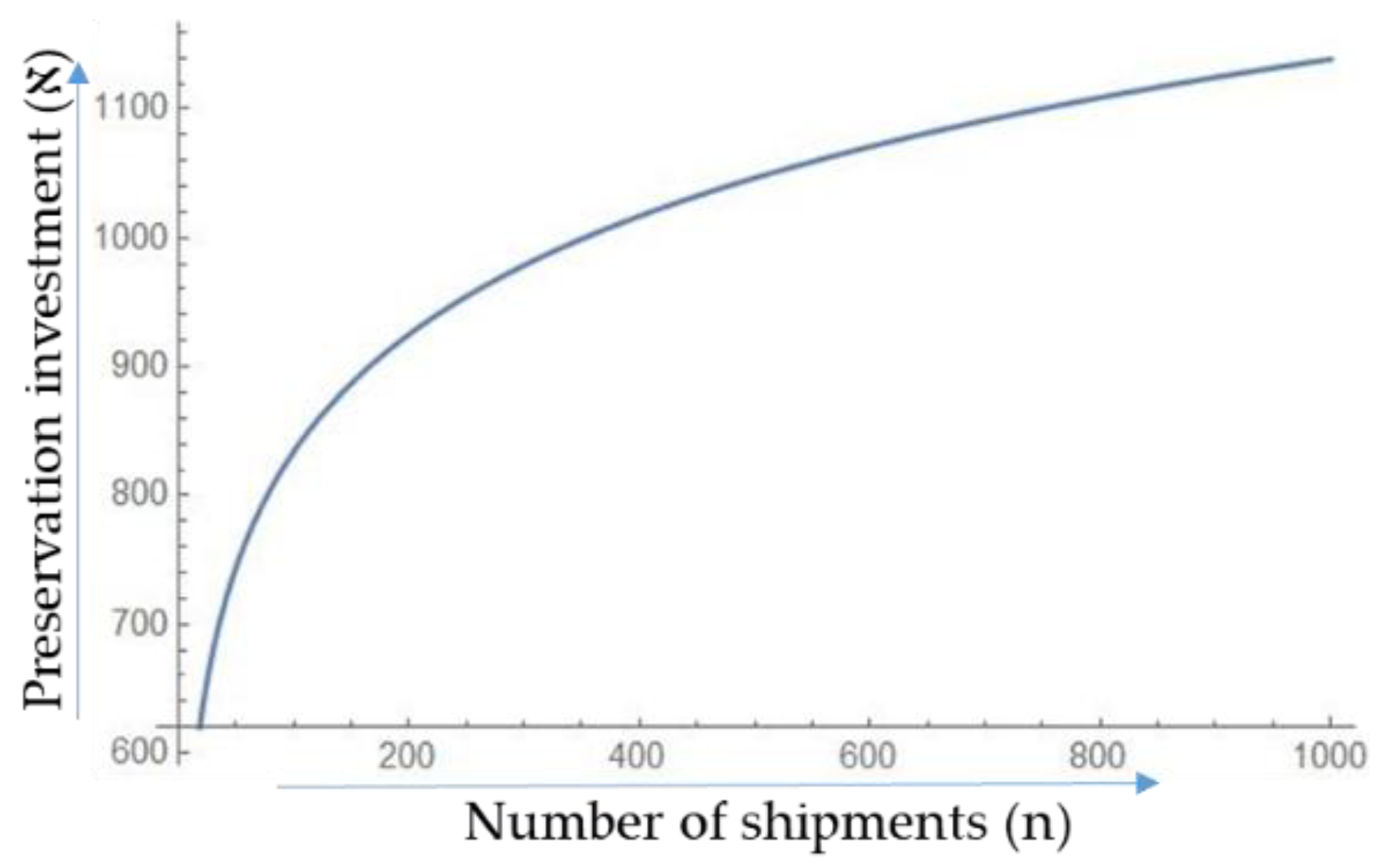For instance, after an investment$\aleph$, the net deterioration rate $\mathsf{\lambda }$changes to$\left(\mathsf{\lambda }-\mathrm{w}\left(\aleph \right)\right).$The reduction rate is expressed as a function of the preservation technology cost $\aleph$, such that $\mathrm{w}\left(\aleph \right)=\mathsf{\lambda }\left(1-{\mathrm{e}}^{-\mathrm{g}\aleph }\right)$, where g is the shape parameter and it shows the effectiveness of the investment on the reduction of deterioration. The deterioration function $\mathrm{w}\left(\aleph \right)$ is monotonically increasing in $\aleph$ and is at least twice differentiable. The relationship between preservation investment and reduction in deterioration rate is graphically illustrated in Figure 1. With a zero investment in preservation technology, the net deterioration rate remains the original deterioration rate$\mathsf{\lambda }$. Whereas, with an increase in investment, the net deterioration rate reduces by a factor of $\mathrm{w}\left(\aleph \right).$

We also consider preservation during transportation in this model for deteriorating items. Which means, the products are transported under special conditions, such as transportation by trucks installed with freezing units. The freezers installed on the truck are also operated by the energy obtained from the truck engine. Accordingly, we consider two types of variable transportation costs; which include the cost of transporting goods and preservation cost during transportation. The retailer’s preservation investment is the cost of maintaining the required freezing conditions during transportation.

3.1.1. Notation

The following notation and assumptions are considered to formulate this model:

Constant demand (units/unit time)	$\mathrm{x}$
Original deterioration rate, $\mathsf{\lambda }>0$ (unit/unit time)	$\mathsf{\lambda }$
Cost of preservation technology, where $\aleph \ge 0$ ($)	$\aleph$
Reduced deterioration rate, a function of $\aleph$ (unit/unit time)	$\mathrm{w}\left(\aleph \right)$
Deterioration cost per unit ($/unit)	${ \mathrm{C}}_{\mathsf{\lambda }}$
Waste disposal cost per deteriorated unit ($/unit)	${ \mathrm{C}}_{\mathrm{d}}$
Inventory cycle length	$\mathrm{T}$
The total cost of the integrated supply chain	$\mathrm{TCSC}$
For manufacturer
Manufacturer’s production rate (unit/unit time)	${\mathrm{p}}_{\mathrm{m}}$
Manufacturer’s setup cost for a production batch ($/batch)	${\mathrm{S}}_{\mathrm{m}}$
Manufacturer’s holding cost ($/unit/unit time)	${\mathrm{h}}_{\mathrm{m}}$
Manufacturer’s production lot size per cycle (units)	$\mathrm{Q}$
Area under the manufacturer’s inventory level	${\Delta }_{\mathrm{m}}$
Manufacturer’s production time duration	${\mathrm{T}}_1$
Manufacturer’s non-production time duration	${\mathrm{T}}_2$
For retailer
Retailer’s ordering cost ($/order)	${\mathrm{A}}_{\mathrm{r}}$
Retailer’s holding cost ($/unit/unit time)	${\mathrm{h}}_{\mathrm{r}}$
Number of deliveries to retailer per production batch (units)	$\mathrm{n}$
Retailer delivery lot size (units)	$\mathrm{q}$
The duration between two successive deliveries to retailer	${\mathrm{T}}_3$
Freezing cost for transportation per unit item per km ($/unit/km)	${\mathrm{F}}_{\mathrm{z}}$
Fixed transportation cost per shipment ($/delivery)	$\mathrm{F}$
Truck capacity (units/truck)	K
Transportation cost per truck unit ($/truck unit)	${\mathrm{c}}_{\mathrm{t}}$
Distance covered (km)	l
Area under the Retailer’s inventory level	${\Delta }_{\mathrm{r}}$

3.1.2. Assumptions

An integrated inventory model is considered, and it is assumed that all information is shared; furthermore, both parties are interested in supply chain coordination. It is assumed that demand is constant and known, and the production rate of the manufacturer is greater than the demand rate. As, ${\mathrm{p}}_{\mathrm{m}}>\mathrm{x}$. The finished product deteriorates at a random rate $\mathsf{\lambda }$, which follows a uniform distribution. All of the deteriorated product is wasted, and supply chain members have to dispose of them properly. The original deterioration is reduced by investing in preservation technology, whereas, the reduction in deterioration is a function of the investment.

The retailer pays the cost of extra preservation during transportation.

4. Mathematical Modeling

In this section, we develop a single setup multiple delivery (SSMD) production model for deteriorating items. The manufacturer produces the production lot in one step but delivers in multiple shipments of a fixed quantity to the retailer at a constant shipment time. To control the deterioration rate of products, the manufacturer invests extra cost$\aleph$ in preservation technology. The total cycle time can be divided into two spans, ${\mathrm{T}}_1{ \mathrm{and} \mathrm{T}}_2$ for the manufacturer. Where${ \mathrm{T}}_1$ is the manufacturer’s production uptime and ${\mathrm{T}}_2$ is the non-production time, in which the manufacturer only makes deliveries to the retailer. The delivery times to the retailer are assigned as each delivery arrives at the time when all items from the previous delivery have been consumed. The supply chain logistics diagram is depicted in Figure 2.

4.1. The Retailer’S Cost

In the proposed system, the retailer needs $\left(\mathrm{Q}=\mathrm{xT}\right)$ quantity to satisfy market demand, for which the retailer incurs $\frac{{\mathrm{A}}_{\mathrm{r}}}{\mathrm{T}}$ ordering cost per cycle. As an SSMD policy is considered, the manufacturer split the lot size into$\mathrm{n}$ equal shipments of size $\mathrm{q}$, such that$\left(\mathrm{Q}=\mathrm{nq}\right)$. However, due to the deteriorating nature of products, the actual shipment size becomes,

$$\mathrm{q}={\mathrm{T}}_3\left(\mathrm{x}+\frac{\left(\mathsf{\lambda }-\mathrm{w}\left(\aleph \right)\mathrm{q}\right)}{2}\right),$$

whereas, ${\mathrm{xT}}_3$ is the market demand and $\left(\frac{\left(\mathsf{\lambda }-\mathrm{w}\left(\aleph \right)\mathrm{q}\right)}{2}\right){\mathrm{T}}_3$ is the expected quantity that deteriorates during time ${\mathrm{T}}_3$. As the retailer cycle time is ${\mathrm{T}}_3=\mathrm{T}/\mathrm{n}$, therfore,

$$\mathrm{q}=\frac{\mathrm{T}}{\mathrm{n}}\left(\mathrm{x}+\frac{\left(\mathsf{\lambda }-\mathrm{w}\left(\aleph \right)\mathrm{q}\right)}{2}\right),$$

and,

$$\frac{\mathrm{n}}{\mathrm{T}}=\frac{\mathrm{q}}{2}\left(\mathsf{\lambda }-\mathrm{w}\left(\aleph \right)\mathrm{q}\right)+\mathrm{x}\Rightarrow \frac{\mathrm{nq}}{\mathrm{T}\left(\mathsf{\lambda }-\mathrm{w}\left(\aleph \right)\mathrm{q}\right)}=\frac{\mathrm{q}}{2}+\frac{\mathrm{x}}{\left(\mathsf{\lambda }-\mathrm{w}\left(\aleph \right)\right)}.$$

Hence, the average inventory of the retailer can be given as,

$$\frac{\mathrm{q}}{2}=\left(\frac{\mathrm{nq}}{\mathrm{T}\left(\mathsf{\lambda }-\mathrm{w}\left(\aleph \right)\right)}-\frac{\mathrm{x}}{\left(\mathsf{\lambda }-\mathrm{w}\left(\aleph \right)\right)}\right).$$

(1)

Total deterioration at the retailer’s end is the difference of total products received and the market demand fulfilled, which can be written as $\left(\mathsf{\lambda }-\mathrm{w}\left(\aleph \right)\right){\Delta }_r=\left(\mathrm{nq}-\mathrm{xT}\right)$. After simplifying, we get the time-weighted average inventory of the retailer, such that,

$$\frac{{\Delta }_{\mathrm{r}}}{\mathrm{T}}=\left(\frac{\mathrm{nq}}{\mathrm{T}\left(\mathsf{\lambda }-\mathrm{w}\left(\aleph \right)\right)}-\frac{\mathrm{x}}{\left(\mathsf{\lambda }-\mathrm{w}\left(\aleph \right)\right)}\right).$$

(2)

From (1) and (2), ${\Delta }_{\mathrm{r}}/\mathrm{T}=\left(\frac{\mathrm{q}}{2}\right)$, therefore, the retailer’s holding cost can be written as $\frac{{\mathrm{h}}_{\mathrm{r}}{\Delta }_{\mathrm{r}}}{\mathrm{T}}$. The retailer average inventory is $\frac{{\Delta }_{\mathrm{r}}}{\mathrm{T}}$, for which the total deterioration cost is $\frac{{\mathrm{C}}_{\mathsf{\lambda }}\left(\mathsf{\lambda }\right){\Delta }_{\mathrm{r}}}{\mathrm{T}}$; however, after the manufacturer’s investment in preservation technology, the net deterioration rate is reduced, for which the total deterioration cost at the retailer ends can be written as $\frac{{\mathrm{C}}_{\mathsf{\lambda }}\left(\mathsf{\lambda }-\mathrm{w}\left(\aleph \right)\right){\Delta }_{\mathrm{r}}}{\mathrm{T}}$. Each deteriorated item needs to be disposed of properly to avoid negative environmental impacts and pollution, for which, the total disposal cost is $\frac{{\mathrm{C}}_{\mathrm{d}}\left(\mathsf{\lambda }-\mathrm{w}\left(\aleph \right)\right){\Delta }_{\mathrm{r}}}{\mathrm{T}}$. It is assumed that transportation is the responsibility of the retailer, and therefore, transportation cost is added to the retailer’s total cost function. The total transportation cost consists of a fixed transportation cost per shipment, the variable transportation cost, and cost of preservation during transportation in terms of freezing, which can be written as $\frac{1}{\mathrm{T}}\left(\mathrm{nF}+\mathrm{nq}\left(\frac{{\mathrm{l}\ast \mathrm{c}}_{\mathrm{t}}}{\mathrm{K}}+{\mathrm{F}}_{\mathrm{z}}\ast \mathrm{l}\right)\right)$. The total cost for the retailer consists of ordering cost, holding cost, deterioration cost, waste disposal cost, and transportation cost, which can be formulated as,

$${\mathrm{TC}}_{\mathrm{r}}=\frac{1}{\mathrm{T}}\left({\mathrm{A}}_{\mathrm{r}}+{\mathrm{h}}_{\mathrm{r}}{\Delta }_{\mathrm{r}}+\left(\mathrm{nF}+\mathrm{nq}\left(\frac{{\mathrm{l}\ast \mathrm{c}}_{\mathrm{t}}}{\mathrm{K}}+{\mathrm{F}}_{\mathrm{z}}\ast \mathrm{l}\right)\right)\right)+({\mathrm{C}}_{\mathrm{d}}+{\mathrm{C}}_{\mathsf{\lambda }}){\Delta }_{\mathrm{r}}\left(\mathsf{\lambda }-\mathrm{w}\left(\aleph \right)\right).$$

Therefore,

$${\mathrm{TC}}_{\mathrm{r}}=\left(\frac{\mathrm{x}}{\mathrm{nq}}+\frac{\mathsf{\lambda }-\mathrm{w}\left(\aleph \right)}{2\mathrm{n}}\right)\left({\mathrm{A}}_{\mathrm{r}}+\left(\mathrm{nF}+\mathrm{nq}\left(\frac{{\mathrm{l}\ast \mathrm{c}}_{\mathrm{t}}}{\mathrm{K}}+{\mathrm{F}}_{\mathrm{z}}\ast \mathrm{l}\right)\right)\right)+\frac{\mathrm{q}}{2}\left({\mathrm{h}}_{\mathrm{r}}+({\mathrm{C}}_{\mathrm{d}}+{\mathrm{C}}_{\mathsf{\lambda }}\right)\left(\mathsf{\lambda }-\mathrm{w}\left(\aleph \right)\right).$$

(3)

4.2. The Manufacturer’S Cost

The manufacturer’s total inventory is calculated with the help of Figure 2. It is clear that the production lot size for the manufacturer is the sum of the retailer demand and the expected number of deteriorated products $\mathrm{r}$ at the manufacturer’s end, such that $\left(\mathrm{Q}=\mathrm{nq}+\mathrm{r}\right).$ With probabilistic deterioration rate $\mathsf{\lambda }$, the number of deteriorating items at the manufacturer’s end is $\left(\mathrm{r}={\mathsf{\lambda }\Delta }_{\mathrm{m}}\right),$ which gives $\left(\frac{\mathrm{r}}{\mathsf{\lambda }}={\Delta }_{\mathrm{m}}\right).$ Therefore, the total number of deteriorated items for the whole supply chain is $\left(\mathrm{r}+\frac{\mathsf{\lambda }\mathrm{qT}}{2}\right)$.

After simplification, we get the manufacturer’s inventory as:

$$\mathrm{r}+\frac{\mathsf{\lambda }\mathrm{qT}}{2}=\mathsf{\lambda }\mathrm{T}\left(\frac{\mathrm{Q}\left(1-\frac{\mathrm{x}}{\mathrm{p}}\right)}{\mathrm{p}}+\frac{\mathrm{xq}}{\mathrm{p}}\right)\Rightarrow {\Delta }_{\mathrm{m}}=\mathrm{qT}\left(\frac{\mathrm{x}}{\mathrm{P}}+\frac{\mathrm{n}-1}{2}-\frac{\mathrm{xn}}{2\mathrm{p}}\right).$$

For $\left(\mathrm{Q}=\mathrm{nq}+\mathrm{r}\right)$ products, the production setup cost for the manufacturer is $\left(\frac{{\mathrm{S}}_{\mathrm{m}}}{\mathrm{T}}\right)$ per cycle. Manufacturer’s holding cost and deterioration cost for average inventory is $\left(\frac{{\mathrm{h}}_{\mathrm{m}}{\Delta }_{\mathrm{m}}}{\mathrm{T}}\right)$ and $\frac{{\mathrm{C}}_{\mathsf{\lambda }}\left(\mathsf{\lambda }\right){\Delta }_{\mathrm{m}}}{\mathrm{T}},$ respectively. With manufacturer’s investment $\aleph$ in preservation technology, the deterioration rate decreases from $\mathsf{\lambda } \mathrm{to} \left(\mathsf{\lambda }-\mathrm{w}\left(\aleph \right)\right)$. Accordingly, the deterioration cost for the manufacturer changes to $\frac{{\mathrm{C}}_{\mathsf{\lambda }}\left(\mathsf{\lambda }-\mathrm{w}\left(\aleph \right)\right){\Delta }_{\mathrm{m}}}{\mathrm{T}}$. The manufacturer also needs to dispose waste generated from net deteriorated items and pays an extra cost of $\frac{{\mathrm{C}}_{\mathrm{d}}\left(\mathsf{\lambda }-\mathrm{w}\left(\aleph \right)\right){\Delta }_{\mathrm{m}}}{\mathrm{T}}.$ The manufacturer’s cost includes setup cost, inventory holding cost, deterioration cost, preservation investment cost, and waste disposal cost, which can be derived as:

$${\mathrm{TC}}_{\mathrm{m}}=\frac{1}{\mathrm{T}}\left({\mathrm{S}}_{\mathrm{m}}+{\mathrm{h}}_{\mathrm{m}}{\Delta }_{\mathrm{m}}+\aleph +({\Delta }_{\mathrm{m}}\left({\mathrm{C}}_{\mathrm{d}}+{\mathrm{C}}_{\mathsf{\lambda }}\right)\left(\mathsf{\lambda }-\mathrm{w}\left(\aleph \right)\right)\right).$$

(4)

Equation (4) can be simplified as given,

$${\mathrm{TC}}_{\mathrm{m}}=\left(\frac{\mathrm{x}}{\mathrm{nq}}+\frac{\left(\mathsf{\lambda }-\mathrm{w}\left(\aleph \right)\right)}{2\mathrm{n}}\right){\mathrm{S}}_{\mathrm{m}}+\aleph +\mathrm{q}\left({\mathrm{h}}_{\mathrm{m}}+({\mathrm{C}}_{\mathrm{d}}+{\mathrm{C}}_{\mathsf{\lambda }}\right)\left(\mathsf{\lambda }-\mathrm{w}\left(\aleph \right)\right)\left(\frac{\mathrm{x}}{\mathrm{p}}+\frac{\mathrm{n}-1}{2}-\frac{\mathrm{xn}}{2\mathrm{p}}\right).$$

(5)

4.3. The Total Supply Chain Cost

The total average cost of the supply chain is the sum of the manufacturer’s and retailer’s individual costs, as follows:

$$\begin{array}{c}\mathrm{TCSC}\left(\mathrm{q},\mathrm{n},\aleph \right)={\mathrm{TC}}_{\mathrm{r}}+{\mathrm{TC}}_{\mathrm{m}}\Rightarrow \left(\frac{\mathrm{x}}{\mathrm{nq}}+\frac{\left(\mathsf{\lambda }-\mathrm{w}\left(\aleph \right)\right)}{2\mathrm{n}}\right)\left({\mathrm{A}}_{\mathrm{r}}+{\mathrm{S}}_{\mathrm{m}}+\left(\mathrm{nF}+\mathrm{nq}\left(\frac{{\mathrm{l}\ast \mathrm{c}}_{\mathrm{t}}}{\mathrm{K}}+{\mathrm{F}}_{\mathrm{z}}\ast \mathrm{l}\right)\right)\right)+ \\ \frac{\mathrm{q}}{2}\left(\left({\mathrm{h}}_{\mathrm{r}}+({\mathrm{C}}_{\mathrm{d}}+{\mathrm{C}}_{\mathsf{\lambda }})\left(\mathsf{\lambda }-\mathrm{w}\left(\aleph \right)\right)\right)+\aleph +\left({\mathrm{h}}_{\mathrm{m}}+({\mathrm{C}}_{\mathrm{d}}+{\mathrm{C}}_{\mathsf{\lambda }})\left(\mathsf{\lambda }-\mathrm{w}\left(\aleph \right)\right)\right)\left(\frac{\left(2-\mathrm{n}\right)\mathrm{x}}{\mathrm{p}}+\mathrm{n}-1\right)\right).\end{array}$$

(6)

In this study, we have considered that the deterioration rate follows a continuous probability distribution function. As $\mathsf{\lambda }=\mathrm{E}\left[\mathrm{f}\left(\mathrm{u}\right)\right]$, with $\mathrm{f}\left(\mathrm{u}\right)$ following a uniform distribution as given below:

$$\mathsf{\lambda }=\mathrm{E}\left[\mathrm{f}\left(\mathrm{u}\right)\right]=\frac{\mathrm{a}+\mathrm{b}}{2}\hspace{1em}\left(\mathrm{a}>0, \mathrm{b}>0, \mathrm{a}<\mathrm{b}\right).$$

Now, the total cost function, Equation (6), can be written as:

$$\begin{array}{c}\mathrm{TCSC}\left(\mathrm{q},\mathrm{n},\aleph \right)=\left(\frac{\mathrm{x}}{\mathrm{nq}}+\left(\frac{\left(\mathrm{a}+\mathrm{b}\right)}{4\mathrm{n}}-\frac{\mathrm{w}\left(\aleph \right)}{2\mathrm{n}}\right)\right)\left({\mathrm{A}}_{\mathrm{r}}+{\mathrm{S}}_{\mathrm{m}}+\left(\mathrm{nF}+\mathrm{nq}\left(\frac{{\mathrm{l}\ast \mathrm{c}}_{\mathrm{t}}}{\mathrm{K}}+{\mathrm{F}}_{\mathrm{z}}\ast \mathrm{l}\right)\right)\right)+\left(\aleph \right)\\ +\frac{\mathrm{q}}{2}\left({\mathrm{h}}_{\mathrm{r}}+\left({\mathrm{C}}_{\mathrm{d}}+{\mathrm{C}}_{\mathsf{\lambda }}\right)\left(\frac{\mathrm{a}+\mathrm{b}}{2}-\mathrm{w}\left(\aleph \right)\right)\right)+\left({\mathrm{h}}_{\mathrm{m}}+({\mathrm{C}}_{\mathrm{d}}+{\mathrm{C}}_{\mathsf{\lambda }})\left(\frac{\mathrm{a}+\mathrm{b}}{2}-\mathrm{w}\left(\aleph \right)\right)\right)\left(\frac{\mathrm{x}\left(2-\mathrm{n}\right)}{\mathrm{p}}+\mathrm{n}-1\right).\end{array}$$

(7)

4.4. Solution Methodology

In this study, we have to find the optimal lot size $\mathrm{q},$ preservation investment $\aleph$, and number of shipments to retailer $\mathrm{n}$. Increasing the investment can control the deterioration rate up to some extent, but after the optimal point, investment contributes more to the total cost of the system compared to the reduction in deteriorated quantity. The objective is to examine the trade-off between the marginal cost of investment and the deteriorated quantities. Besides, a large order size q may increase the deteriorated quantity, yet, low order quantity would increase the ordering cost and transportation cost. A classical optimization technique is used to determine the optimal shipment quantity, number of shipments, and optimal investment in deterioration reduction. The developed problem consists of both continuous variables $\mathrm{q}$ and $\aleph$ and discrete variable $\mathrm{n}$, which makes the model a MINLP problem. Due to the complexity of the objective function, it is impossible to solve it with ordinary optimization techniques. Therefore, this section provides a solution methodology to solve the problem and obtain the optimal policies for the proposed system.

Assuming that the lot size q and preservation investment ℵ are any real nonzero numbers, then, at fixed n, there exists a unique q and ℵ, that minimizes the total cost and satisfies the following first-order conditions (FOC);

$$\begin{array}{c}\frac{\partial \left(\mathrm{TCSC}\left(\mathrm{q},\mathrm{n},\aleph \right)\right)}{\partial \left(\mathrm{q}\right)}\hfill \\ = \frac{\mathsf{\pi }+\left(\mathrm{a}+\mathrm{b}\right){\mathrm{e}}^{-\mathrm{g}\aleph }\left(\mathrm{p}\left(\left(\frac{{\mathrm{l}\ast \mathrm{c}}_{\mathrm{t}}}{\mathrm{K}}+{\mathrm{F}}_{\mathrm{z}}\ast \mathrm{l}\right)\mathrm{nq}+{\mathrm{nC}}_{\mathrm{d}}\right)+{\mathrm{C}}_{\mathsf{\lambda }}\mathrm{n}\left(\mathrm{p}-\mathrm{x}\right)+2{\mathrm{C}}_{\mathsf{\lambda }}\mathrm{x}-{\mathrm{C}}_{\mathrm{d}}\mathrm{x}\left(\mathrm{n}-2\right)\right)}{4\mathrm{p}}\hfill \\ =0,\hfill \end{array}$$

(8)

where, $\mathsf{\pi } = 2{\mathrm{h}}_{\mathrm{r}}\mathrm{p}-\frac{4\left({\mathrm{A}}_{\mathrm{r}}+{\mathrm{S}}_{\mathrm{m}}+\mathrm{nF}\right)\mathrm{px}}{{\mathrm{nq}}^2}-2{\mathrm{h}}_{\mathrm{m}}\left(\mathrm{p}-\mathrm{np}+\left(\mathrm{n}-2\right)\mathrm{x}\right),$

and,

$$\begin{array}{c}\frac{\partial \left(\mathrm{TCSC}\left(\mathrm{q},\mathrm{n},\aleph \right)\right)}{\partial \left(\aleph \right)} = 1-\frac{\left(\mathrm{a}+\mathrm{b}\right){\mathrm{S}}_{\mathrm{m}}{\mathrm{e}}^{-\mathrm{g}\aleph }\mathrm{g}}{4\mathrm{n}}-\frac{\left(\mathrm{a}+\mathrm{b}\right){\mathrm{e}}^{-\mathrm{g}\aleph }\mathrm{g} ({\mathrm{A}}_{\mathrm{r}}+\left(\mathrm{nF}+\left(\frac{{\mathrm{l}\ast \mathrm{c}}_{\mathrm{t}}}{\mathrm{K}}+{\mathrm{F}}_{\mathrm{z}}\ast \mathrm{l}\right)\mathrm{nq}\right)}{4\mathrm{n}}\\ -\frac{1}{4}\left(\mathrm{a}+\mathrm{b}\right){\mathrm{e}}^{-\mathrm{g}\aleph }\mathrm{g}\mathrm{q}\left({\mathrm{C}}_{\mathrm{d}}+{\mathrm{C}}_{\mathsf{\lambda }}\right)-\frac{1}{2}\left(\mathrm{a}+\mathrm{b}\right){\mathrm{e}}^{-\mathrm{g}\aleph }\mathrm{g}\mathrm{q}\left({\mathrm{C}}_{\mathrm{d}}+{\mathrm{C}}_{\mathsf{\lambda }}\right)\left(\frac{1}{2}\left(\mathrm{n}-1\right)+\frac{\mathrm{x}}{\mathrm{p}}-\frac{\mathrm{nx}}{2\mathrm{p}}\right)=0\end{array}$$

(9)

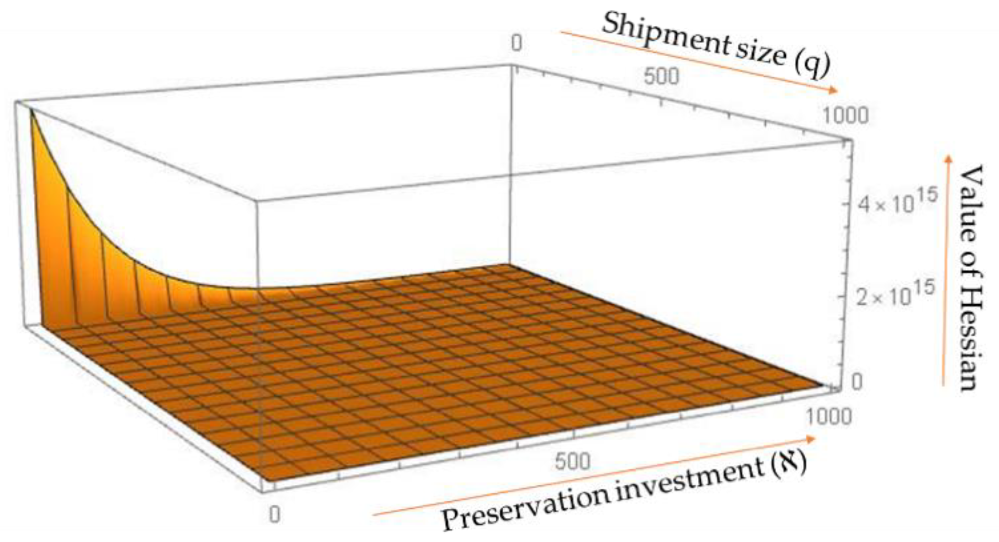
Furthermore, $\mathrm{TCSC}\left(\mathrm{q},\mathrm{n},\aleph \right)$ is convex, if at ${\mathrm{q}}^{\ast }$ and ${\aleph }^{\ast },$ the Hessian of $\mathrm{TCSC}\left(\mathrm{q},\mathrm{n},\aleph \right)$ is positive semidefinite. The convexity proof of the solution is provided in Appendix A.

As the number of shipments $\mathrm{n}$ is a discrete variable, the optimal number of shipments can be determined using the following necessary condition which ${\mathrm{n}}^{\ast }$ has to satisfy; for the optimal total cost

$\mathrm{TCSC}$ at $\mathrm{q}={\mathrm{q}}^{\ast }$ and $\aleph ={\aleph }^{\ast }$, the necessary condition is,

$$\mathrm{TCSC}\left({\mathrm{q}}^{\ast }, {\aleph }^{\ast },{\mathrm{n}}^{\ast }-1\right) \ge \mathrm{TCSC}\left({\mathrm{q}}^{\ast }, {\aleph }^{\ast },{ \mathrm{n}}^{\ast }\right)\le \mathrm{TCSC}\left({\mathrm{q}}^{\ast }, {\aleph }^{\ast },{\mathrm{n}}^{\ast }+1\right)$$

And the optimal value of ${\mathrm{n}}^{\ast }$ is driven by Equation (10),

$$\frac{1}{2}\left(\mathsf{\gamma }-1\right)\le \mathrm{n}\le \frac{1}{2}\left(\mathsf{\gamma }+1\right),$$

(10)

where,

$$\mathsf{\gamma }=\frac{\left(\sqrt{{\mathrm{q}}^2\left({\mathrm{h}}_{\mathrm{m}}+\mathsf{\lambda }\left({\mathrm{C}}_{\mathrm{d}}+{\mathrm{C}}_{\mathsf{\lambda }}\right)\right)\left(\mathrm{p}-\mathrm{x}\right)+4{\mathrm{A}}_{\mathrm{r}}\mathrm{p}\left(\mathsf{\lambda }\mathrm{q}+2\mathrm{x}\right)+4{\mathrm{S}}_{\mathrm{m}}\mathrm{p}\left(\mathsf{\lambda }\mathrm{q}+2\mathrm{x}\right)-\mathrm{q}\left(4{\mathrm{A}}_{\mathrm{r}}\mathrm{p}+4{\mathrm{S}}_{\mathrm{m}}\mathrm{p}+\mathrm{q}\left({\mathrm{C}}_{\mathrm{d}}+{\mathrm{C}}_{\mathsf{\lambda }}\right)\left(\mathrm{p}-\mathrm{x}\right)\right)\mathrm{w}\left(\aleph \right)}\right)}{(\mathrm{q}\surd \left(\mathrm{p}-\mathrm{x}\right) \surd \left({\mathrm{h}}_{\mathrm{m}}+\mathsf{\lambda }\left({\mathrm{C}}_{\mathrm{d}}+{\mathrm{C}}_{\mathsf{\lambda }}\right)-\left({\mathrm{C}}_{\mathrm{d}}+{\mathrm{C}}_{\mathsf{\lambda }}\right)\mathrm{w}\left(\aleph \right)\right))}.$$

Solution algorithm

Step 1. Set $\mathrm{n}$ = 1 and $\aleph =0$, find ${\mathrm{q}}^{\ast }$ from FOC (8)

Step 1.1. Using $\mathrm{q}={\mathrm{q}}^{\ast }$, find ${\aleph }^{\ast }$ from FOC (9)

Step 1.2. Using $\aleph ={\aleph }^{\ast }$, find ${\mathrm{q}}^{\ast }$ from FOC (8)

Step 1.3. Repeat Step 1.1 and 1.2 until values of ${\aleph }^{\ast }$, find ${\mathrm{q}}^{\ast }$ stop changing, update ${\aleph }^{\ast }$, find ${\mathrm{q}}^{\ast }$ as optimal values at fixed $\mathrm{n}$.

Step 1.4. Find the total cost $\mathrm{TCSC}\left({\mathrm{q}}^{\ast }, {\aleph }^{\ast },\mathrm{n}\right)$ from (7). $\mathrm{TCSC}\left({\mathrm{q}}^{\ast }, {\aleph }^{\ast },\mathrm{n}\right)$ is an optimal solution at fixed $\mathrm{n}.$

Step 2. Set ${\mathrm{n}}^{\ast }=n+1$, perform Step 1.1 to 1.4.

Step 2.1. If $\mathrm{TCSC}\left({\mathrm{q}}^{\ast }, {\aleph }^{\ast },\mathrm{n}\right)\le$ $\mathrm{TCSC}\left({\mathrm{q}}^{\ast }, {\aleph }^{\ast },\mathrm{n}-1\right)$ go to Step 2., else go to Step 3.

Step 3. Set ${\mathrm{n}}^{\ast }=n-1$, $\mathrm{TCSC}\left({\mathrm{q}}^{\ast }, {\aleph }^{\ast },\mathrm{n}\right)$ is the optimal solution.

5. Numerical Experiment

To get a deeper insight into the total costs and preservation technology investment relationship, we consider a numerical example with two cases in this section. The first case is the proposed model developed in the previous section. The second case considers a manufacturer that does not consider preservation investment, and consequently, the model reduces to two decision variables, with ℵ = $0.

Case1:

The first case considers the preservation investment from the manufacturer’s side. The data, taken from Sarkar [17], is given below with appropriate units.

A_r = $25/order, S_m = $800/batch, C_λ = $40/unit, C_d = $10/unit, F = $50/shipment, h_r = $7/unit/year, h_m = $6/unit/year, p = 10,000 units/year, c_t = $0.05/truck unit, K = 200 units/truck, F_z = $0.00225/unit/truck, l = 400, x = 4800 units/year, g = 0.0075, a = 0.15, b = 0.25.

The optimal results with preservation investment are $\mathrm{q}=261.7 \mathrm{units},\aleph =\$492.5/\mathrm{Cycle},\mathrm{n}=6/\mathrm{Cycle}$, with the total cost of the system $\mathrm{TCSC}=\$121,99.5/\mathrm{Cycle}$.

Case2:

In the second case of the given example, a manufacturer is considered who does not invest in preservation technology. The model is solved with the same data, and preservation investment is consider as $\aleph =\$0$. Then, the optimal solution without preservation investment is $\mathrm{TCSC}=“\$”13,906.05/\mathrm{Cycle},\mathrm{q}=202.2 \mathrm{units},\mathrm{n}=6/\mathrm{Cycle}$. Results of both cases are compiled in

Table 1. Optimal results of case 1 and case 2.

Model	q (Units)	n (Shipments)	ℵ ($)	TCSC ($)	Generated Waste (Units)
With preservation investment	261.7	6	492.5	12,199.5	$\left(\mathsf{\lambda }-\mathsf{\lambda }\left(1-{\mathrm{e}}^{-\mathrm{g}\aleph }\right)\right)\mathrm{nq}$ = 7.76
Without preservation investment	202.2	6	0	13,906.05	$\left(\mathsf{\lambda }-\mathsf{\lambda }\left(1-{\mathrm{e}}^{-\mathrm{g}\aleph }\right)\right)\mathrm{nq}$ = 235.46

.

As shown in Table 1, the optimal lot size is $\mathrm{q}=261.7$ units with preservation investment, and without preservation investment, the lot size reduces to $\mathrm{q}=202.2$ units. The shipment size for both cases remains six shipments/ cycle. We also observe, that with an investment of $\left(\aleph =\$492.5/\mathrm{cycle}\right)$ the total cost of model TCSC reduces 13% from $\$13,906.05 \mathrm{to} \$12,199.5$.

5.1. Sensitivity Analysis

To gain a deeper understanding of cost drivers in the proposed supply chain, sensitivity analysis is performed by varying the values of the input parameters within the range [−50% +50%]. The results of sensitivity analysis are compiled in

Table 2. Sensitivity analysis of input parameters.

Parameter	% Change in Value	Decision Variables			% Change in Total Cost
		q	ℵ	n
${\mathrm{A}}_{\mathrm{r}}$	−50	261.70	491.70	6	−0.32
	−25	261.70	492.14	6	−0.16
	+25	261.70	492.90	6	0.16
	+50	261.70	493.30	7	0.31
${\mathrm{S}}_{\mathrm{m}}$	−50	260.40	459.60	5	−11.77
	−25	261.20	478.40	5	−5.39
	+25	262.10	503.80	7	4.76
	+50	262.4	513.3	8	9.07
${\mathrm{C}}_{\mathsf{\lambda }}$	−50	261.6	425.2	6	−0.55
	−25	261.7	463.1	6	−0.24
	+25	261.70	516.6	6	0.20
	+50	261.70	537.1	6	0.37
F	−50	184.80	482.40	8	−4.41
	−25	226.50	488.00	7	−2.02
	+25	292.70	496.30	5	1.77
	+50	320.8	499.7	5	3.38
${\mathrm{h}}_{\mathrm{r}}$	−50	371.00	505.50	4	−4.40
	−25	302.40	497.50	5	−2.02
	+25	234.00	489.00	7	1.77
	+50	213.60	486.30	8	3.38
${\mathrm{h}}_{\mathrm{m}}$	−50	260.50	527.50	9	−11.51
	−25	261.00	506.70	7	−5.28
	+25	262.40	481.80	6	4.66
	+50	263.20	473.30	5	8.87
${\mathrm{c}}_{\mathrm{t}}$	−50	261.70	492.20	6	−1.97
	−25	261.74	492.95	6	−0.98
	+25	261.70	492.55	6	0.99
	+50	261.70	492.56	6	1.97
${\mathrm{F}}_{\mathrm{z}}$	−50	261.77	492.24	6	−17.70
	−25	261.76	492.39	6	−8.85
	+25	261.72	492.68	6	8.86
	+50	261.70	492.83	6	17.71
g	−50	247.9	119.4	6	3.61
	−25	260.1	604.4	6	1.29
	+25	262.6	418.2	6	−0.83
	+50	263.3	364.9	6	−1.42

.

It is clear from sensitivity results that the total cost of the system is highly sensitive to the variable cost of transportation ${\mathrm{c}}_{\mathrm{t}}$.

The freezing cost per unit item during transportation has the highest impact on total cost; up to 50% reduction in it, decreases the total cost by 18%. Even though this cost has a high impact on the total cost of the system, it does not affect the decision variables in any significant way.

The second most significant parameter regarding total cost variation is the manufacturer’s holding cost. A 50% reduction in it decreases the total cost by 11.5%. Although, manufacturing holding cost does not change shipment size, however, its increment decreases production lot size by decreasing the number of shipments. Furthermore, it also reduces investment in preservation technology.

Although the retailer’s holding cost affects the total cost, it has more influence on the number of shipments and shipment size. For a higher retailer’s holding cost, the number of shipments increases and the shipment size decreases.

Constant transportation cost has the highest influence on the number of shipments. An increase in constant transportation cost decreases the shipment size considerably.

The most relevant parameter regarding investment in preservation, is the shape parameter g. Increasing the shape parameter increases the effectiveness of the technology and, hence, preservation investment is reduced.

A 50% increase in the manufacturer’s setup cost increases the total cost by 10%. An increase in this cost leads to an increase in the number of shipments per cycle, which results in a decrease in the number of setups per year.

Although, deterioration per unit item does not affect total cost to a large extent, its effect on preservation investment is enormous. The decrease in deterioration cost decreases investment in preservation and vice versa. The effect of waste disposal cost is similar to deterioration cost, the more disposal cost per unit the deteriorated item has, the more investment is required.

5.2. Comparative Study

The comparative study shows the relationship between decision variables with total cost and their inter-relationship. It shows how the optimal value of a decision variable and total cost changes with changing the value of other decision variables.

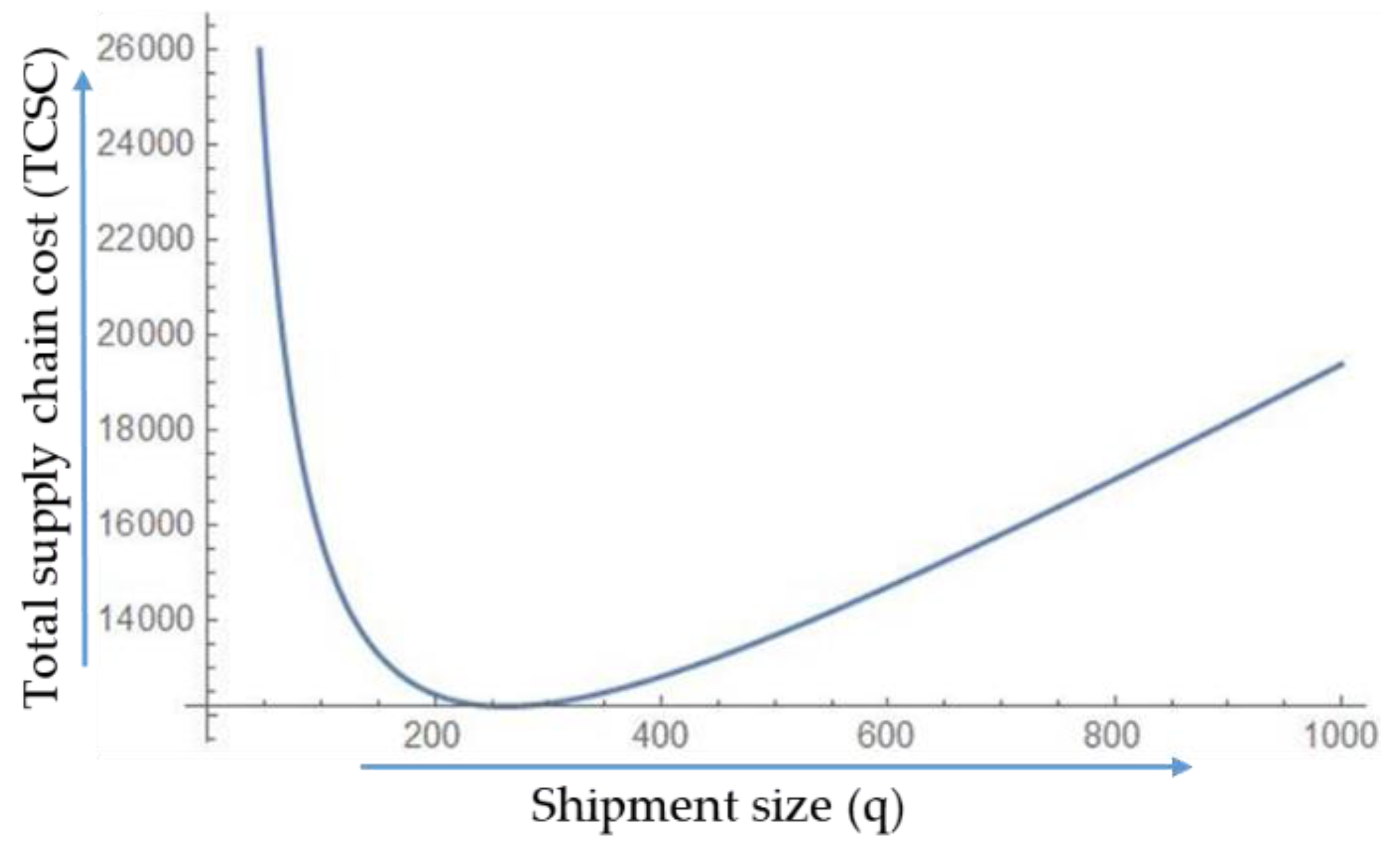
5.2.1. Relationship of Total Cost with Decision Variables

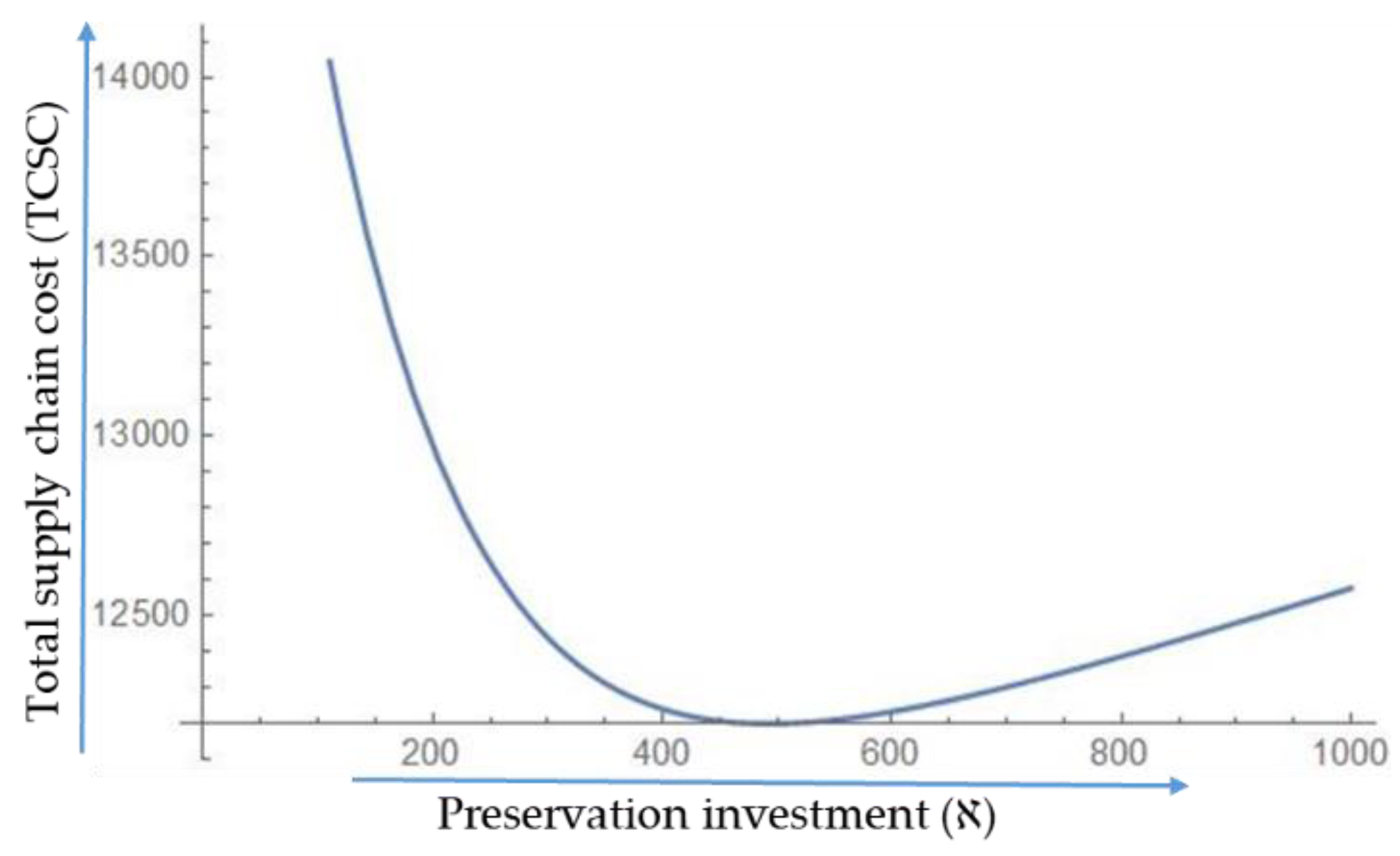
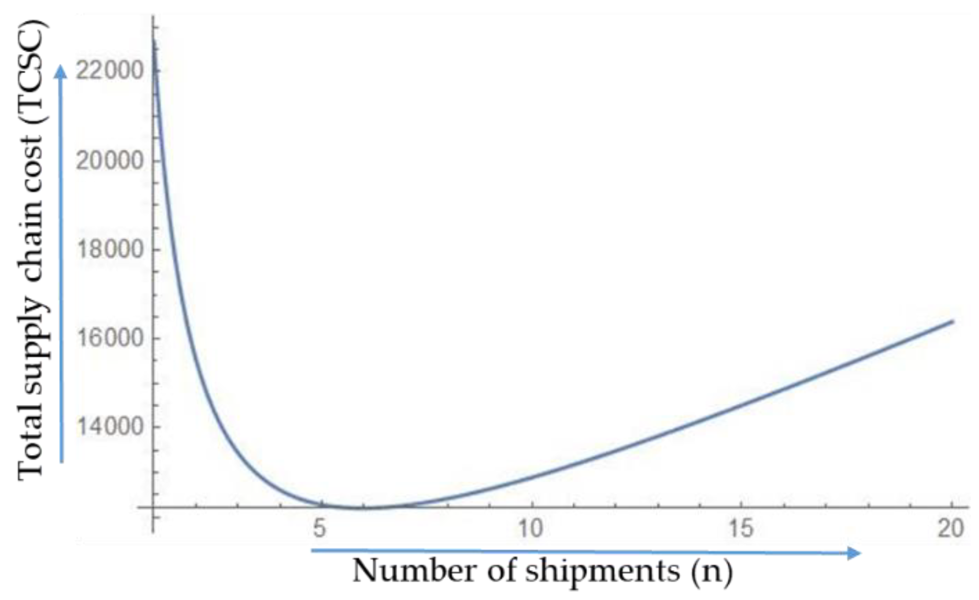
The impact of shipment size q on total cost is illustrated in Figure 3. It is clear that total cost increases with both an increase and decrease in the optimal value of q. Figure 4 shows the convexity of the objective function with preservation investment when other parameters are constant. Similarly, Figure 5 provides the impact of variation in shipment frequency on the total cost of the system.

5.2.2. Inter-Relationship of Decision Variables

In this section, we develop the comparative study of decision variables. Figure 6 shows the impact of investment parameter $\aleph$ on the optimal lot size $\mathrm{q}$; with the increase in investment, the lot size increases as well.

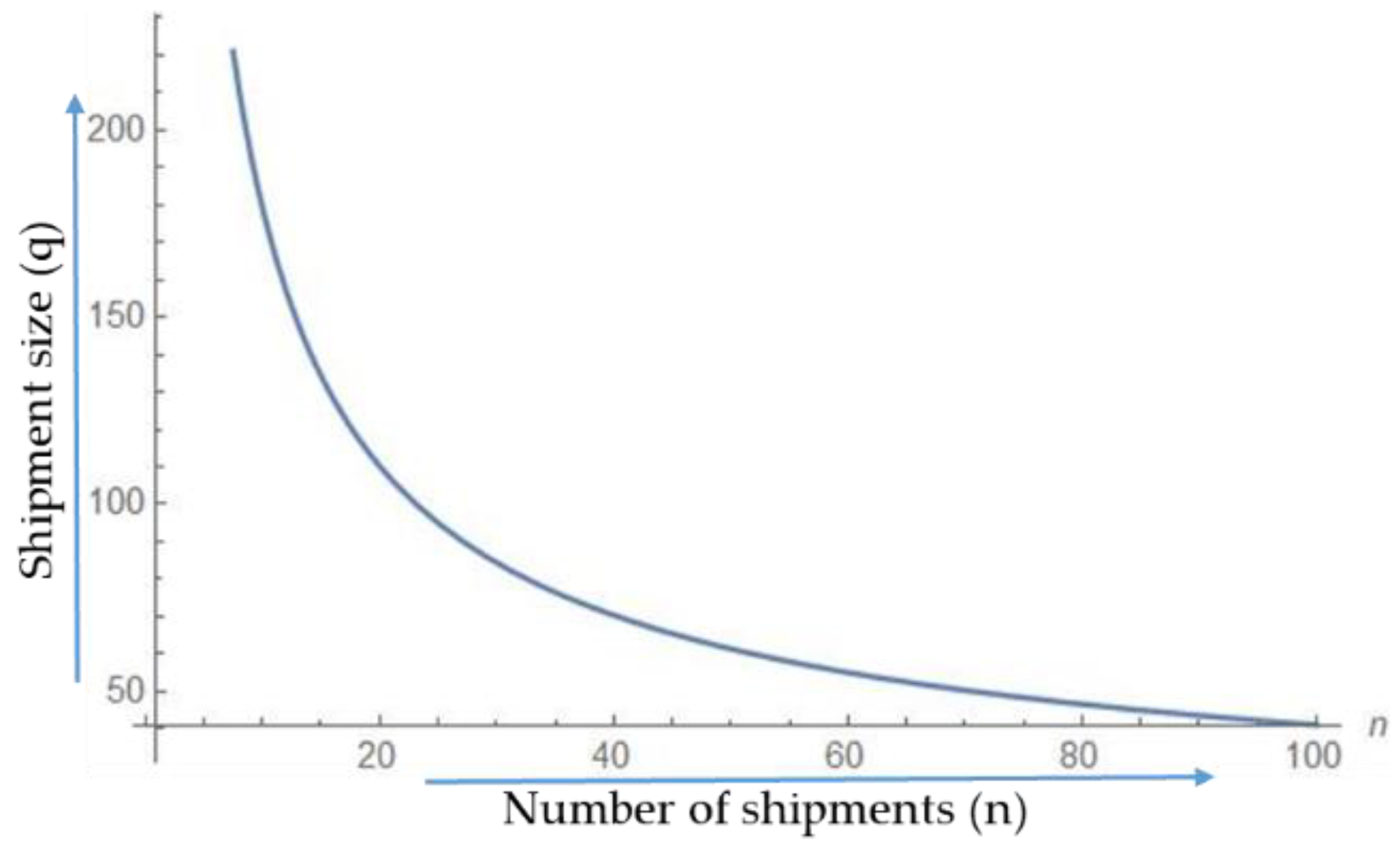
Figure 7 shows the impact of the number of shipments $\mathrm{n}$ on the optimal lot size $\mathrm{q}$; as the number of shipments is increased, the shipment lot size decreases accordingly.

Figure 8 shows the impact of shipments size $\mathrm{q}$ on the optimal preservation investment $\aleph$; as the shipment quantity increases, the preservation investments needs to be increased respectively.

Figure 9 shows the impact of shipment frequency $\mathrm{n}$ on the optimal preservation investment $\aleph$; increasing shipment frequency increases the production lot size, which increases the required preservation investments.

Figure 10 shows the impact of shipments quantity $\mathrm{q}$ on the optimal number of shipments $\mathrm{n}$. This relation is obvious, as increasing the shipment frequency would decrease the time between two shipments, thus reducing shipment size.

Figure 11 shows the impact of preservation investment $\aleph$ on the optimal number of shipments $\mathrm{n}$; as the preservation investment increases, the shipment frequency increases consequently.

5.3. Managerial Insights

• Several important managerial insights are drawn from the sensitivity analysis and comparative study to assist supply chain managers in decision making.
• Supply chain managers should consider the investment in preservation technology; as it not only reduces the total cost, but also decreases waste generation in the supply chain. The results of our study confer a high decrease in the amount of product loss and generated waste with preservation and encouraged investment for deterioration prevention strategies. Without preservation, the firm faces product shortages because of deterioration, in addition, extra waste disposal cost adds up in a system.
• The sensitivity analysis represents the amount of preservation investment decrease with a decrease in the effectiveness of the technology. It also shows that the preservation cost for products depends on their deterioration cost per unit. Consequently, a product with more monetary value and high deterioration cost needs higher preservation investments. However, the total cost of the supply chain increases with a decrease in preservation investment. Therefore, supply chain managers are suggested to consider the deterioration cost of specific products and the most effective preservation technology accordingly.
• The results further showed that preservation leads to an increase in the optimal lot size, which consequently decreases the number of orders per year and ordering cost per year in a supply chain. Managers should consider the ordering costs for products in deciding the investment plans for preservation technology, as higher preservation investment may be required for products that have higher ordering costs in a supply chain.
• Also, the optimal size of shipments increases in a supply chain with an increase in deterioration prevention investment. Hence, supply chain managers should consider preservation investment to increase shipment size instead of shipment frequency, especially when transportation costs are high for the system.
• Another important parameter that should be considered by managers is the retailer holding cost. The higher holding cost of the retailer increases the number of shipments, and hence, increases the transportation cost per year of the supply chain. Furthermore, it also reduces the optimal lot size, which increases the ordering cost of the retailer. Hence, investment in deterioration prevention is crucial for supply chain management with a higher holding cost at the retailer’s end.
• Finally, this study suggests that supply chain managers should regulate the environmental and financial impacts of their supply chain networks through deterioration prevention techniques. As with preservation investment, the quantity of decayed/deteriorated products reduces, and the consumption of resources also reduces which makes preservation technology a concluding sustainable approach for perishable products.

6. Conclusions

Product deterioration compromises the ability of any firm to achieve its economic and environmental goals. Economically, firms face extra manufacturing costs to catch up the shortage faced by deterioration. While, environmentally, product deterioration causes extra resource consumption that has no beneficiary output for manufacturing firms, the deteriorated items also cause pollution and landfills backlash. Deteriorating products in a multi-firm network multiply the loss, as deterioration occurs at every stage of the supply chain network. This study extended the existing literature on stochastic deteriorating inventory models in supply chain management with preservation technology investment in production and transportation. A two-echelon supply chain is considered, where the deterioration rate of integrated inventory follows a continuous probability distribution. This paper considered investments in preservation technology by the manufacturer to control the deterioration rate and solid waste generation, and its impacts on supply chain were studied. The retailer considers the transportation of products under a particular condition to increase the effectiveness of the preservation technology. For instance, refrigerated transportation is adopted by the retailer, which means the deteriorating products are transported by the vehicle installed with freezing units. Both parties properly dispose of the waste generated from deteriorating items and endure waste disposal costs.

The tradeoff between preservation investment in supply chain performance is very promising. The results showed that investing in preservation technology reduces the total cost of the system by 13%, because of the controlled deterioration rate and reduced deteriorated products in both the manufacturer’s and retailer’s inventories. Furthermore, preservation technology reduces waste generation in the proposed supply chain from 235 to 8 deteriorated products per cycle. In the proposed supply chain, these results confer a high decrease in the amount of product loss and generated waste. This also leads to improving the environmental performance of the supply chain. The results further showed that investment in the preservation leads to an increase in the optimal lot size q, hence decreasing the number of orders per year, which reduces the ordering cost per year. This suggests that preservation investment is even more beneficial in supply chains where product ordering costs are high. Also, the optimal size of shipments increases with an increase in deterioration prevention investment. Hence, for a supply chain with high transportation costs, preservation investment is necessary to increase shipment size instead of shipment frequency.

The sensitivity analysis shows that the preservation cost for products depends on their deterioration cost per unit. Deterioration cost per unit symbolizes the commercial value of products and also the cost of replacing a product in the given setup. Consequently, a product with more monetary value and high deterioration cost needs higher preservation investments as well. It was also found from sensitivity analysis, that an increase in buyer holding cost increases the number of shipments, and hence, increases the transportation cost per year. Furthermore, it also reduces the optimal lot size, which increases the ordering cost of the retailer. Hence, investment in deterioration prevention is crucial for supply chain management with a higher holding cost at the retailer’s end. The managerial insights help supply chain managers to decide on the required amount of investment and the type of technology for considered deteriorating products. The model can be extended to the multi-item supply chain system with different preservation investment policies. Stochastic or seasonal demand can be another possible extension, as for deteriorating items, demand usually varies with time. Another possible extension is considering shared or joint preservation practices in resilient supply chain management, a comprehensive example is provided by Mari et al. [45] with disruption risks.