A High-Order Convex Splitting Method for a Non-Additive Cahn–Hilliard Energy Functional

Abstract

Various Cahn–Hilliard (CH) energy functionals have been introduced to model phase separation in multi-component system. Mathematically consistent models have highly nonlinear terms linked together, thus it is not well-known how to split this type of energy. In this paper, we propose a new convex splitting and a constrained Convex Splitting (cCS) scheme based on the splitting. We show analytically that the cCS scheme is mass conserving and satisfies the partition of unity constraint at the next time level. It is uniquely solvable and energy stable. Furthermore, we combine the convex splitting with the specially designed implicit–explicit Runge–Kutta method to develop a high-order (up to third-order) cCS scheme for the multi-component CH system. We also show analytically that the high-order cCS scheme is unconditionally energy stable. Numerical experiments with ternary and quaternary systems are presented, demonstrating the accuracy, energy stability, and capability of the proposed high-order cCS scheme.

1. Introduction

The Cahn–Hilliard (CH) equation was originally introduced as a phenomenological model of phase separation in a binary alloy [1] and has been applied to a wide range of problems [2]. The CH equation is derived from the Ginzburg–Landau energy functional:

$${\mathcal{E}}_{\mathrm{GL}}\left(c\right):={\int }_{\mathsf{\Omega }}\left(\frac{w}{2}{c}^2{(1-c)}^2+\frac{{ϵ}^2}{2}{|\nabla c|}^2\right)d\mathbf{x},$$

where c is the concentration field defined in $\mathsf{\Omega }(\subset {\mathbb{R}}^d,d=1,2,3)$ and $w,ϵ>0$ are the free energy and gradient energy coefficients. The CH equation is a gradient flow for ${\mathcal{E}}_{\mathrm{GL}}\left(c\right)$ in the $H^{-1}$-inner product, thus ${\mathcal{E}}_{\mathrm{GL}}\left(c\right)$ is nonincreasing in time.

Generalizations of ${\mathcal{E}}_{\mathrm{GL}}\left(c\right)$ for more than two components can be applied to wide range of problems, thus have been studied intensively [3,4,5,6,7,8,9,10,11,12,13,14,15,16,17]. A great deal of research has been focused on the ternary system [10] such as:

$${\mathcal{E}}_{\mathrm{FP}}(c_1,c_2,c_3):={\int }_{\mathsf{\Omega }}\left(\frac{w}{2}\sum _{i=1}^3{c}_i^2{(1-c_i)}^2+\frac{{ϵ}^2}{2}\sum _{i=1}^3{|\nabla c_i|}^2\right)d\mathbf{x},$$

where $c_i$ is the concentration field of the phase i. There are many other forms of energy functional for the ternary system and some of them are equivalent. For example, under the constraint $c_1+c_2+c_3=1$, the first term in ${\mathcal{E}}_{\mathrm{FP}}(c_1,c_2,c_3)$ can be rewritten [11] as follows:

$$\frac{w}{2}\sum _{i=1}^3{c}_i^2{(1-c_i)}^2=w\left(c_1^2{c}_2^2+c_1^2{c}_3^2+c_2^2{c}_3^2+c_1{c}_2{c}_3\right).$$

One of the most important criteria for the multi-component model is to avoid the generation of spurious phases. To be more precise, we think a physically reasonable model must satisfy the following two fundamental criteria:

(A) 

(Consistency of null-phase) If a phase is absent at the initial time, it should not appear at any time.

(B) 

(No additional phase on interface) The interface including multiple junction should be free of additional phases.

The model with ${\mathcal{E}}_{\mathrm{FP}}(c_1,c_2,c_3)$ and many other models with three components obey both criteria; however, it is not well-known how to construct an energy functional for more than three components satisfying mathematical and physical criteria including these two. For example, the following generalization introduced by Lee and Kim [12] for the vector-valued concentration field $\mathbf{c}={(c_1,\dots ,c_N)}^T$:

$${\mathcal{E}}_{\mathrm{LK}}\left(\mathbf{c}\right):={\int }_{\mathsf{\Omega }}\left(\frac{w}{2}\sum _{i=1}^N{c}_i^2{(1-c_i)}^2+\frac{{ϵ}^2}{2}\sum _{i=1}^N{|\nabla c_i|}^2\right)d\mathbf{x}$$

does not satisfy Criteria A and B when $N>3$.

In this paper, we consider the following energy functional satisfying Criteria A and B:

$$\mathcal{E}\left(\mathbf{c}\right):={\int }_{\mathsf{\Omega }}\left(wF\left(\mathbf{c}\right)+\frac{{ϵ}^2}{2}\sum _{i=1}^N{|\nabla c_i|}^2\right)d\mathbf{x},$$

(1)

where

$$F\left(\mathbf{c}\right)=\frac{1}{12}+\sum _{i=1}^N\left(\frac{c_i^4}{4}-\frac{c_i^3}{3}\right)+\frac{1}{2}\sum _{i=1}^N\sum _{j=i+1}^N{c}_i^2{c}_j^2.$$

The energy functional $\mathcal{E}\left(\mathbf{c}\right)$ introduced by Tóth et al. [14] is a non-trivial extension of ${\mathcal{E}}_{\mathrm{GL}}\left(c\right)$ for more than three component system in the sense that it is equivalent to ${\mathcal{E}}_{\mathrm{FP}}(c_1,c_2,c_3)$ when $N=3$ and ${\mathcal{E}}_{\mathrm{GL}}\left(c\right)$ when $N<3$. We develop a high-order energy stable numerical method for this energy with quadratically mixed terms ${\sum }_{i<j}{c}_i^2{c}_j^2$ to study phase separation in multi-component systems.

The $H^{-1}$-gradient flow for $\mathcal{E}\left(\mathbf{c}\right)$ is given by

$$\begin{array}{cc}\hfill & \frac{\partial \mathbf{c}}{\partial t}=\Delta \mathit{\mu },\mathit{\mu }:=\frac{\delta \mathcal{E}}{\delta \mathbf{c}}=w\left(\frac{\partial F}{\partial \mathbf{c}}+\alpha \left(\mathbf{c}\right)\mathbf{1}\right)-{ϵ}^2\Delta \mathbf{c},\hfill \end{array}$$

(2)

under the partition of unity constraint,

$$c_1+\cdots +c_N=1,$$

(3)

where $\mathit{\mu }={({\mu }_1,\dots ,{\mu }_N)}^T$ is the vector-valued chemical potential, ${\mu }_i$ is the chemical potential of the phase i, $\frac{\delta }{\delta \mathbf{c}}$ denotes the variational derivative with respect to $\mathbf{c}$, $\frac{\partial F}{\partial \mathbf{c}}={\left(\frac{\partial F}{\partial c_1},\dots ,\frac{\partial F}{\partial c_N}\right)}^T$, $\frac{\partial F}{\partial c_i}=-c_i^2+c_i{\sum }_{j=1}^N{c}_j^2$, $\alpha \left(\mathbf{c}\right)=-\frac{1}{N}{\sum }_{i=1}^N\frac{\partial F}{\partial c_i}$ is a Lagrange multiplier to ensure the constraint [8,10,11,12,13,16,17], and $\mathbf{1}={(1,\dots ,1)}^T$∈${\mathbb{R}}^N$. We consider the boundary conditions for $c_i$ and ${\mu }_i$ as the zero Neumann boundary conditions:

$$\nabla c_i·\mathbf{n}=\nabla {\mu }_i·\mathbf{n}=0\mathrm{on}\partial \mathsf{\Omega },$$

where $\mathbf{n}$ is a unit normal vector to $\partial \mathsf{\Omega }$. We refer to Equation (2) as the vector-valued CH (vCH) equation. Because the vCH equation is of gradient type, $\mathcal{E}\left(\mathbf{c}\right)$ is nonincreasing in time as the constraint holds:

$$\begin{array}{ccc}\hfill \frac{d\mathcal{E}}{dt}& =& {\int }_{\mathsf{\Omega }}\sum _{i=1}^N\left(w\frac{\partial F}{\partial c_i}\frac{\partial c_i}{\partial t}+{ϵ}^2\nabla c_i·\nabla \frac{\partial c_i}{\partial t}\right)d\mathbf{x}={\int }_{\mathsf{\Omega }}\sum _{i=1}^N\left(w\frac{\partial F}{\partial c_i}-{ϵ}^2\Delta c_i\right)\frac{\partial c_i}{\partial t}d\mathbf{x}\hfill \\ & =& {\int }_{\mathsf{\Omega }}\sum _{i=1}^N\left({\mu }_i-w\alpha \left(\mathbf{c}\right)\right)\frac{\partial c_i}{\partial t}d\mathbf{x}={\int }_{\mathsf{\Omega }}\sum _{i=1}^N{\mu }_i\Delta {\mu }_{i}d\mathbf{x}-{\int }_{\mathsf{\Omega }}w\alpha \left(\mathbf{c}\right)\frac{\partial }{\partial t}\sum _{i=1}^N{c}_{i}d\mathbf{x}\hfill \\ & =& -{\int }_{\mathsf{\Omega }}\sum _{i=1}^N{|\nabla {\mu }_i|}^{2}d\mathbf{x}\le 0.\hfill \end{array}$$

The vCH equation is a fourth-order nonlinear partial differential equation and the N unknowns $c_1,\dots ,c_N$ are linked through the constraint. Therefore, accurate and efficient numerical methods are desirable to study the dynamics of the vCH equation. In this paper, we propose a constrained Convex Splitting (cCS) scheme for the vCH equation, which is based on a convex splitting of $\mathcal{E}\left(\mathbf{c}\right)$ under the constraint. For $N=2$ and 3, $\mathcal{E}\left(\mathbf{c}\right)$ has a straightforward convex–concave splitting. However, there is a difficulty with $N>3$ since ${\int }_{\mathsf{\Omega }}wF\left(\mathbf{c}\right)d\mathbf{x}$ in $\mathcal{E}\left(\mathbf{c}\right)$ is neither convex nor concave. To apply the convex splitting idea [18,19,20] for all N, we add and subtract an auxiliary term in $\mathcal{E}\left(\mathbf{c}\right)$. Then, a convex–concave decomposition is available. We show analytically that the cCS scheme is mass conserving and satisfies the constraint at the next time level. It is uniquely solvable and energy stable. Furthermore, we combine the convex splitting with the implicit–explicit Runge–Kutta (RK) method [21,22] to develop a high-order (up to third-order) cCS scheme. We employ the specially designed implicit–explicit RK tables [23] to have both high-order time accuracy and unconditional energy stability. We also show analytically that the high-order cCS scheme is unconditionally energy stable.

This paper is organized as follows. In Section 2, we describe the convex splitting with an auxiliary term. We propose the (first-order) cCS scheme for the vCH equation and prove its unconditional unique solvability and energy stability. In Section 3, we construct the high-order cCS scheme with a proof of unconditional energy stability. In Section 4, we present numerical examples showing the accuracy, energy stability, and capability of the proposed scheme. Finally, conclusions are drawn in Section 5.

2. Constrained Convex Splitting Scheme

The convex splitting of $\mathcal{E}\left(\mathbf{c}\right)$ when $N<3$ is trivial; however, it is not well-known how to split $\mathcal{E}\left(\mathbf{c}\right)$ for $N\ge 3$ into convex and concave parts. Therefore, we here propose to split $\mathcal{E}\left(\mathbf{c}\right)$ for $N\ge 3$ according to $\mathcal{E}\left(\mathbf{c}\right)={\mathcal{E}}_c\left(\mathbf{c}\right)-{\mathcal{E}}_e\left(\mathbf{c}\right)$ with

$${\mathcal{E}}_c\left(\mathbf{c}\right)={\int }_{\mathsf{\Omega }}\left(w{F}_c\left(\mathbf{c}\right)+\frac{{ϵ}^2}{2}\sum _{i=1}^N{|\nabla c_i|}^2\right)d\mathbf{x},{\mathcal{E}}_e\left(\mathbf{c}\right)={\int }_{\mathsf{\Omega }}w{F}_e\left(\mathbf{c}\right)d\mathbf{x},$$

(4)

where

$$\begin{array}{ccc}\hfill F_c\left(\mathbf{c}\right)& =& \frac{1}{12}+\frac{1}{4}\sum _{i=1}^N\sum _{j=i+1}^N{(c_i^2+c_j^2)}^2+\sum _{i=1}^N\frac{c_i^2}{6(N-2)},\hfill \\ \hfill F_e\left(\mathbf{c}\right)& =& \sum _{i=1}^N\left(\frac{(N-2)c_i^4}{4}+\frac{c_i^3}{3}+\frac{c_i^2}{6(N-2)}\right).\hfill \end{array}$$

Lemma 1.

Both ${\mathcal{E}}_c\left(\mathbf{c}\right)$ and ${\mathcal{E}}_e\left(\mathbf{c}\right)$ in (4) are convex.

Proof. 

For any $\mathbf{d}\in H_0=\left\{{(d_1,\dots ,d_N)}^T|{\sum }_{i=1}^N{d}_i=0,{\int }_{\mathsf{\Omega }}{d}_{i}d\mathbf{x}=0\mathrm{for}i=1,\dots ,N\right\}$,

$$\begin{array}{ccc}\hfill {\mathcal{E}}_c(\mathbf{c}+\eta \mathbf{d})& =& {\mathcal{E}}_c\left(\mathbf{c}\right)+\eta {\int }_{\mathsf{\Omega }}\left(w\left(\frac{\partial F_c\left(\mathbf{c}\right)}{\partial \mathbf{c}}+{\alpha }_c\left(\mathbf{c}\right)\mathbf{1}\right)-{ϵ}^2\Delta \mathbf{c}\right)·\mathbf{d}d\mathbf{x}\hfill \\ & & +\frac{{\eta }^2}{2}{\int }_{\mathsf{\Omega }}\left(w{\mathbf{d}}^T\mathbf{H}\left(F_c\left(\mathbf{c}\right)\right)\mathbf{d}+\sum _{i=1}^N{ϵ}^2{|\nabla d_i|}^2\right)d\mathbf{x}+O\left({\eta }^3\right),\hfill \end{array}$$

where ${\alpha }_c\left(\mathbf{c}\right)=-\frac{1}{N}{\sum }_{i=1}^N\frac{\partial F_c\left(\mathbf{c}\right)}{\partial c_i}$, $\mathbf{H}\left(F_c\left(\mathbf{c}\right)\right)$ is the Hessian matrix of $F_c\left(\mathbf{c}\right)$, and

$$\mathbf{H}{\left(F_c\left(\mathbf{c}\right)\right)}_{ij}=\frac{{\partial }^2{F}_c\left(\mathbf{c}\right)}{\partial c_i\partial c_j}={\left(\left(\sum _{j=1}^N{c}_j^2+3(N-2)c_i^2+\frac{1}{3(N-2)}\right)\mathbf{I}+2\mathbf{c}{\mathbf{c}}^T\right)}_{ij}.$$

From the positive semi-definiteness of $\mathbf{H}\left(F_c\left(\mathbf{c}\right)\right)$, we obtain

$${\left.\frac{d^2{\mathcal{E}}_c(\mathbf{c}+\eta \mathbf{d})}{d{\eta }^2}\right|}_{\eta =0}={\int }_{\mathsf{\Omega }}\left(w{\mathbf{d}}^T\mathbf{H}\left(F_c\left(\mathbf{c}\right)\right)\mathbf{d}+\sum _{i=1}^N{ϵ}^2{|\nabla d_i|}^2\right)d\mathbf{x}\ge 0.$$

For ${\mathcal{E}}_e\left(\mathbf{c}\right)$,

$$\begin{array}{ccc}\hfill {\mathcal{E}}_e(\mathbf{c}+\eta \mathbf{d})& =& {\mathcal{E}}_e\left(\mathbf{c}\right)+\eta {\int }_{\mathsf{\Omega }}w\left(\frac{\partial F_e\left(\mathbf{c}\right)}{\partial \mathbf{c}}+{\alpha }_e\left(\mathbf{c}\right)\mathbf{1}\right)·\mathbf{d}d\mathbf{x}\hfill \\ & & +\frac{{\eta }^2}{2}{\int }_{\mathsf{\Omega }}w\sum _{i=1}^N\frac{{\partial }^2{F}_e\left(\mathbf{c}\right)}{\partial c_i^2}{d}_i^{2}d\mathbf{x}+O\left({\eta }^3\right),\hfill \end{array}$$

where ${\alpha }_e\left(\mathbf{c}\right)=-\frac{1}{N}{\sum }_{i=1}^N\frac{\partial F_e\left(\mathbf{c}\right)}{\partial c_i}$. Then, we have

$$\begin{array}{ccc}\hfill {\left.\frac{d^2{\mathcal{E}}_e(\mathbf{c}+\eta \mathbf{d})}{d{\eta }^2}\right|}_{\eta =0}& =& {\int }_{\mathsf{\Omega }}w\sum _{i=1}^N\frac{{\partial }^2{F}_e\left(\mathbf{c}\right)}{\partial c_i^2}{d}_i^{2}d\mathbf{x}\hfill \\ & =& {\int }_{\mathsf{\Omega }}w\sum _{i=1}^{N}3(N-2){\left(c_i+\frac{1}{3(N-2)}\right)}^2{d}_i^{2}d\mathbf{x}\ge 0.\hfill \end{array}$$

Thus, the convexity of ${\mathcal{E}}_c\left(\varphi \right)$ and ${\mathcal{E}}_e\left(\varphi \right)$ is assured. □

We now present the cCS scheme for the vCH Equation (2) by treating ${\mathcal{E}}_c\left(\mathbf{c}\right)$ implicitly and ${\mathcal{E}}_e\left(\mathbf{c}\right)$ explicitly under the partition of unity constraint in Equation (3):

$$\begin{array}{cc}\hfill \frac{{\mathbf{c}}^{n+1}-{\mathbf{c}}^n}{\Delta t}& =\Delta {\mathit{\mu }}^{n+1},\hfill \\ \hfill {\mathit{\mu }}^{n+1}:& =\frac{\delta {\mathcal{E}}_c\left({\mathbf{c}}^{n+1}\right)}{\delta \mathbf{c}}-\frac{\delta {\mathcal{E}}_e\left({\mathbf{c}}^n\right)}{\delta \mathbf{c}}\hfill \\ & =w\left(\frac{\partial F_c\left({\mathbf{c}}^{n+1}\right)}{\partial \mathbf{c}}+{\alpha }_c\left({\mathbf{c}}^{n+1}\right)\mathbf{1}\right)-{ϵ}^2\Delta {\mathbf{c}}^{n+1}-w\left(\frac{\partial F_e\left({\mathbf{c}}^n\right)}{\partial \mathbf{c}}+{\alpha }_e\left({\mathbf{c}}^n\right)\mathbf{1}\right),\hfill \end{array}$$

(5)

where $\frac{\partial F_c}{\partial \mathbf{c}}={\left(\frac{\partial F_c}{\partial c_1},\dots ,\frac{\partial F_c}{\partial c_N}\right)}^T$, $\frac{\partial F_c}{\partial c_i}=c_i{\sum }_{j=1}^N{c}_j^2+(N-2)c_i^3+\frac{c_i}{3(N-2)}$, $\frac{\partial F_e}{\partial \mathbf{c}}={\left(\frac{\partial F_e}{\partial c_1},\dots ,\frac{\partial F_e}{\partial c_N}\right)}^T$, and $\frac{\partial F_e}{\partial c_i}=(N-2)c_i^3+c_i^2+\frac{c_i}{3(N-2)}$.

Lemma 2.

The cCS scheme in Equation (5) is mass conserving.

Proof. 

Let ${\mathbf{c}}^{n+1}$ be a solution of the cCS scheme. From Equation (5), we have

$${\int }_{\mathsf{\Omega }}(c_i^{n+1}-c_i^n)d\mathbf{x}=\Delta t{\int }_{\mathsf{\Omega }}\Delta {\mu }_i^{n+1}d\mathbf{x}=\Delta t{\int }_{\partial \mathsf{\Omega }}\nabla {\mu }_i^{n+1}·\mathbf{n}ds=0,$$

where we used the zero Neumann boundary condition for ${\mu }_i$. It follows that ${\int }_{\mathsf{\Omega }}{c}_i^{n+1}d\mathbf{x}={\int }_{\mathsf{\Omega }}{c}_i^{n}d\mathbf{x}$.  □

Lemma 3.

The cCS scheme satisfies the constraint at any time $t^n$, i.e., ${\sum }_{i=1}^N{c}_i^n=1$ if an initial condition satisfies ${\sum }_{i=1}^N{c}_i^0=1$.

Proof. 

Since ${\sum }_{i=1}^N\frac{\partial F_c\left({\mathbf{c}}^{n+1}\right)}{\partial c_i}+N{\alpha }_c\left({\mathbf{c}}^{n+1}\right)=0$ and ${\sum }_{i=1}^N\frac{\partial F_e\left({\mathbf{c}}^n\right)}{\partial c_i}+N{\alpha }_e\left({\mathbf{c}}^n\right)=0$, we have from Equation (5)

$$\begin{array}{c}\frac{1}{\Delta t}\sum _{i=1}^N(c_i^{n+1}-c_i^n)=-{ϵ}^2{\Delta }^2\sum _{i=1}^N{c}_i^{n+1},\hfill \\ \mathrm{i}.\mathrm{e}.,(\mathcal{I}+\Delta t{ϵ}^2{\Delta }^2)\sum _{i=1}^N{c}_i^{n+1}=\sum _{i=1}^N{c}_i^n,\hfill \end{array}$$

(6)

where $\mathcal{I}$ denotes the identity operator. Since $\mathcal{I}+\Delta t{ϵ}^2{\Delta }^2$ with the zero Neumann boundary condition for $c_i$ is an invertible operator, Equation (6) has a unique solution. Thus, Equation (6) ensures that ${\sum }_{i=1}^N{c}_i^{n+1}=1$ for all $n\ge 0$ with the initial condition satisfying ${\sum }_{i=1}^N{c}_i^0=1$. □

Theorem 1.

The cCS scheme with an initial condition satisfying ${\sum }_{i=1}^N{c}_i^0=1$ is uniquely solvable for any time step $\Delta t>0$.

Proof. 

We consider the following functional on $\tilde{H}=\left\{\mathbf{c}|{\sum }_{i=1}^N{c}_i=1,{\int }_{\mathsf{\Omega }}{c}_{i}d\mathbf{x}={\int }_{\mathsf{\Omega }}{c}_i^{n}d\mathbf{x}\mathrm{for}i=1,\dots ,N\right\}$:

$$\mathcal{G}\left(\mathbf{c}\right)=\frac{1}{2\Delta t}{\parallel \mathbf{c}-{\mathbf{c}}^n\parallel }_{H^{-1}}^2+{\mathcal{E}}_c\left(\mathbf{c}\right)-{\left(\frac{\delta {\mathcal{E}}_e\left({\mathbf{c}}^n\right)}{\delta \mathbf{c}},\mathbf{c}\right)}_{L^2},$$

where ${(·,·)}_{H^{-1}}$ and ${(·,·)}_{L^2}$ denote the $H^{-1}$- and $L^2$-inner products, respectively, and ${\left(-\Delta \mathbf{c},\mathbf{d}\right)}_{H^{-1}}={\left(\mathbf{c},\mathbf{d}\right)}_{L^2}={\int }_{\mathsf{\Omega }}\mathbf{c}·\mathbf{d}d\mathbf{x}$ (we refer to [24] for the definition of the $H^{-1}$-inner product). It may be shown that ${\mathbf{c}}^{n+1}\in \tilde{H}$ is the unique minimizer of $\mathcal{G}\left(\mathbf{c}\right)$ if and only if it solves, for any $\mathbf{d}\in H_0$,

$$\begin{array}{ccc}\hfill {\left.\frac{d\mathcal{G}(\mathbf{c}+\eta \mathbf{d})}{d\eta }\right|}_{\eta =0}& =& {\left(\frac{\mathbf{c}-{\mathbf{c}}^n}{\Delta t},\mathbf{d}\right)}_{H^{-1}}+{\left(\frac{\delta {\mathcal{E}}_c\left(\mathbf{c}\right)}{\delta \mathbf{c}},\mathbf{d}\right)}_{L^2}-{\left(\frac{\delta {\mathcal{E}}_e\left({\mathbf{c}}^n\right)}{\delta \mathbf{c}},\mathbf{d}\right)}_{L^2}\hfill \\ & =& {\left(\frac{\mathbf{c}-{\mathbf{c}}^n}{\Delta t}-\Delta \left(\frac{\delta {\mathcal{E}}_c\left(\mathbf{c}\right)}{\delta \mathbf{c}}-\frac{\delta {\mathcal{E}}_e\left({\mathbf{c}}^n\right)}{\delta \mathbf{c}}\right),\mathbf{d}\right)}_{H^{-1}}=0,\hfill \end{array}$$

(7)

because $\mathcal{G}\left(\mathbf{c}\right)$ is strictly convex by the convexity of ${\mathcal{E}}_c\left(\mathbf{c}\right)$. Equation (7) is true for any $\mathbf{d}\in H_0$ if and only if Equation (5) holds. Hence, minimizing the strictly convex functional $\mathcal{G}\left(\mathbf{c}\right)$ is equivalent to solving Equation (5). □

Lemma 4.

The convexity of ${\mathcal{E}}_c\left(\mathbf{c}\right)$ and ${\mathcal{E}}_e\left(\mathbf{c}\right)$ yields the following inequality:

$$\mathcal{E}\left(\mathbf{c}\right)-\mathcal{E}\left(\mathbf{d}\right)\le {\left(\frac{\delta {\mathcal{E}}_c\left(\mathbf{c}\right)}{\delta \mathbf{c}}-\frac{\delta {\mathcal{E}}_e\left(\mathbf{d}\right)}{\delta \mathbf{c}},\mathbf{c}-\mathbf{d}\right)}_{L^2}.$$

(8)

Proof. 

Since both ${\mathcal{E}}_c\left(\mathbf{c}\right)$ and ${\mathcal{E}}_e\left(\mathbf{c}\right)$ are convex, we obtain

$${\mathcal{E}}_c\left(\mathbf{c}\right)-{\mathcal{E}}_c\left(\mathbf{d}\right)\le {\left(\frac{\delta {\mathcal{E}}_c\left(\mathbf{c}\right)}{\delta \mathbf{c}},\mathbf{c}-\mathbf{d}\right)}_{L^2},{\mathcal{E}}_e\left(\mathbf{c}\right)-{\mathcal{E}}_e\left(\mathbf{d}\right)\ge {\left(\frac{\delta {\mathcal{E}}_e\left(\mathbf{d}\right)}{\delta \mathbf{c}},\mathbf{c}-\mathbf{d}\right)}_{L^2}.$$

Subtracting these inequalities yields

$$\begin{array}{ccc}\hfill \mathcal{E}\left(\mathbf{c}\right)-\mathcal{E}\left(\mathbf{d}\right)& =& {\mathcal{E}}_c\left(\mathbf{c}\right)-{\mathcal{E}}_e\left(\mathbf{c}\right)-({\mathcal{E}}_c\left(\mathbf{d}\right)-{\mathcal{E}}_e\left(\mathbf{d}\right))\hfill \\ & \le & {\left(\frac{\delta {\mathcal{E}}_c\left(\mathbf{c}\right)}{\delta \mathbf{c}},\mathbf{c}-\mathbf{d}\right)}_{L^2}-{\left(\frac{\delta {\mathcal{E}}_e\left(\mathbf{d}\right)}{\delta \mathbf{c}},\mathbf{c}-\mathbf{d}\right)}_{L^2}\hfill \\ & =& {\left(\frac{\delta {\mathcal{E}}_c\left(\mathbf{c}\right)}{\delta \mathbf{c}}-\frac{\delta {\mathcal{E}}_e\left(\mathbf{d}\right)}{\delta \mathbf{c}},\mathbf{c}-\mathbf{d}\right)}_{L^2}.\hfill \end{array}$$

□

Theorem 2.

The cCS scheme with an initial condition satisfying ${\sum }_{i=1}^N{c}_i^0=1$ is unconditionally energy stable, meaning that, for any $\Delta t>0$,

$$\mathcal{E}\left({\mathbf{c}}^{n+1}\right)\le \mathcal{E}\left({\mathbf{c}}^n\right).$$

Proof. 

Setting $\mathbf{c}={\mathbf{c}}^{n+1}$ and $\mathbf{d}={\mathbf{c}}^n$ in Equation (8), we have

$$\begin{array}{ccc}\hfill \mathcal{E}\left({\mathbf{c}}^{n+1}\right)-\mathcal{E}\left({\mathbf{c}}^n\right)& \le & {\left(\frac{\delta {\mathcal{E}}_c\left({\mathbf{c}}^{n+1}\right)}{\delta \mathbf{c}}-\frac{\delta {\mathcal{E}}_e\left({\mathbf{c}}^n\right)}{\delta \mathbf{c}},{\mathbf{c}}^{n+1}-{\mathbf{c}}^n\right)}_{L^2}\hfill \\ & =& \Delta t{\left({\mathit{\mu }}^{n+1},\Delta {\mathit{\mu }}^{n+1}\right)}_{L^2}=-\Delta t{\left(\nabla {\mathit{\mu }}^{n+1},\nabla {\mathit{\mu }}^{n+1}\right)}_{L^2}\le 0.\hfill \end{array}$$

□

3. Extension of the Constrained Convex Splitting Scheme To High-Order Time Accuracy

The cCS scheme in Equation (5),

$$\frac{{\mathbf{c}}^{n+1}-{\mathbf{c}}^n}{\Delta t}=\Delta \frac{\delta {\mathcal{E}}_c\left({\mathbf{c}}^{n+1}\right)}{\delta \mathbf{c}}-\Delta \frac{\delta {\mathcal{E}}_e\left({\mathbf{c}}^n\right)}{\delta \mathbf{c}},$$

is first-order accurate in time and its order of time accuracy can be improved by various approaches. One of them is to combine with an s-stage implicit–explicit RK method [21]: let ${\mathbf{c}}^{\left(0\right)}={\mathbf{c}}^n$,

$${\mathbf{c}}^{\left(k\right)}={\mathbf{c}}^{\left(0\right)}+\Delta t\sum _{l=1}^k\left(a_{kl}\Delta \frac{\delta {\mathcal{E}}_c\left({\mathbf{c}}^{\left(l\right)}\right)}{\delta \mathbf{c}}-{\widehat{a}}_{k,l-1}\Delta \frac{\delta {\mathcal{E}}_e\left({\mathbf{c}}^{(l-1)}\right)}{\delta \mathbf{c}}\right),$$

(9)

where $a_{kl}$ and ${\widehat{a}}_{kl}$ are RK coefficients for $k=1,\dots ,s$, and then

$${\mathbf{c}}^{n+1}={\mathbf{c}}^{\left(s\right)}$$

by using the stiffly accurate condition.

Recently, the authors of [23] proved that a Convex Splitting Runge–Kutta scheme for a gradient flow is unconditionally energy stable under the resemble condition ($a_{kl}={\widehat{a}}_{k,l-1}=r_{kl}$ for $k=1,\dots ,s$ and $l=1,\dots ,k$). Applying the resemble condition to Equation (9), we have the following s-stage high-order cCS scheme for the vCH equation (2):

$${\mathbf{c}}^{\left(k\right)}={\mathbf{c}}^{\left(0\right)}+\Delta t\sum _{l=1}^k{r}_{kl}\Delta {\mathit{\mu }}^{\left(l\right)},\mathrm{for}k=1,\dots ,s,$$

(10)

where ${\mathit{\mu }}^{\left(l\right)}:=\frac{\delta {\mathcal{E}}_c\left({\mathbf{c}}^{\left(l\right)}\right)}{\delta \mathbf{c}}-\frac{\delta {\mathcal{E}}_e\left({\mathbf{c}}^{(l-1)}\right)}{\delta \mathbf{c}}=w\left(\frac{\partial F_c\left({\mathbf{c}}^{\left(l\right)}\right)}{\partial \mathbf{c}}+{\alpha }_c\left({\mathbf{c}}^{\left(l\right)}\right)\mathbf{1}\right)-{ϵ}^2\Delta {\mathbf{c}}^{\left(l\right)}-w\left(\frac{\partial F_e\left({\mathbf{c}}^{(l-1)}\right)}{\partial \mathbf{c}}+{\alpha }_e\left({\mathbf{c}}^{(l-1)}\right)\mathbf{1}\right)$.

Lemma 5.

The s-stage high-order cCS scheme in Equation (10) is also mass conserving, satisfies the constraint at any time $t^n$, and is uniquely solvable for any time step $\Delta t>0$, provided that $r_{kk}\ge 0$ for $k=1,\dots ,s$.

Proof. 

The proofs are similar to Lemmas 2 and 3 and Theorem 1, thus we omit the details here. □

Before proving the energy stability of the s-stage high-order cCS scheme, we define an $s\times s$ matrix $\mathbf{R}$ as ${\mathbf{R}}_{kl}=r_{kl}$ for $l\le k$ and ${\mathbf{R}}_{kl}=0$ for $l>k$, and an $s\times s$ matrix $\tilde{\mathbf{R}}$ as ${\tilde{\mathbf{R}}}_{kl}={\tilde{r}}_{kl}=r_{kl}-r_{k-1,l}$ with $r_{0l}=0$.

Theorem 3.

Suppose that $\tilde{\mathbf{R}}$ is positive definite. The s-stage high-order cCS scheme with $r_{kk}\ge 0$ for $k=1,\dots ,s$ and an initial condition satisfying ${\sum }_{i=1}^N{c}_i^0=1$ is unconditionally energy stable, meaning that for any $\Delta t>0$,

$$\mathcal{E}\left({\mathbf{c}}^{n+1}\right)\le \mathcal{E}\left({\mathbf{c}}^n\right).$$

Proof. 

The analogous proof can be found in [23]. Using Lemma 4, we have

$$\begin{array}{ccc}\hfill \mathcal{E}\left({\mathbf{c}}^{n+1}\right)-\mathcal{E}\left({\mathbf{c}}^n\right)& =& \sum _{k=1}^s\left(\mathcal{E}\left({\mathbf{c}}^{\left(k\right)}\right)-\mathcal{E}\left({\mathbf{c}}^{(k-1)}\right)\right)\hfill \\ & \le & \sum _{k=1}^s{\left(\frac{\delta {\mathcal{E}}_c\left({\mathbf{c}}^{\left(k\right)}\right)}{\delta \mathbf{c}}-\frac{\delta {\mathcal{E}}_e\left({\mathbf{c}}^{(k-1)}\right)}{\delta \mathbf{c}},{\mathbf{c}}^{\left(k\right)}-{\mathbf{c}}^{(k-1)}\right)}_{L^2}\hfill \\ & =& \Delta t\sum _{k=1}^s{\left({\mathit{\mu }}^{\left(k\right)},\sum _{l=1}^k{\tilde{r}}_{kl}\Delta {\mathit{\mu }}^{\left(l\right)}\right)}_{L^2},\hfill \end{array}$$

where the last equality follows from the fact that

$$\begin{array}{ccc}\hfill {\mathbf{c}}^{\left(k\right)}-{\mathbf{c}}^{(k-1)}& =& \Delta t\left(\sum _{l=1}^k{r}_{kl}\Delta {\mathit{\mu }}^{\left(l\right)}-\sum _{l=1}^{k-1}{r}_{k-1,l}\Delta {\mathit{\mu }}^{\left(l\right)}\right)\hfill \\ & =& \Delta t\left(\sum _{l=1}^k(r_{kl}-r_{k-1,l})\Delta {\mathit{\mu }}^{\left(l\right)}+r_{k-1,k}\Delta {\mathit{\mu }}^{\left(k\right)}\right)\hfill \\ & =& \Delta t\sum _{l=1}^k(r_{kl}-r_{k-1,l})\Delta {\mathit{\mu }}^{\left(l\right)}=\Delta t\sum _{l=1}^k{\tilde{r}}_{kl}\Delta {\mathit{\mu }}^{\left(l\right)}.\hfill \end{array}$$

Let $\nabla \mathit{\mu }={(\nabla {\mathit{\mu }}^{\left(1\right)},\dots ,\nabla {\mathit{\mu }}^{\left(s\right)})}^T$. Since $\tilde{\mathbf{R}}$ is positive definite,

$$\mathcal{E}\left({\mathbf{c}}^{n+1}\right)-\mathcal{E}\left({\mathbf{c}}^n\right)\le -\Delta t{\left(\nabla \mathit{\mu },\tilde{\mathbf{R}}\nabla \mathit{\mu }\right)}_s\le 0,$$

where ${\left(\mathit{\varphi },\mathit{\psi }\right)}_s={\sum }_{k=1}^s{\left({\mathit{\varphi }}^{\left(k\right)},{\mathit{\psi }}^{\left(k\right)}\right)}_{L^2}$ for $\mathit{\varphi }={({\mathit{\varphi }}^{\left(1\right)},\dots ,{\mathit{\varphi }}^{\left(s\right)})}^T$ and $\mathit{\psi }={({\mathit{\psi }}^{\left(1\right)},\dots ,{\mathit{\psi }}^{\left(s\right)})}^T$. It follows that $\mathcal{E}\left({\mathbf{c}}^{n+1}\right)\le \mathcal{E}\left({\mathbf{c}}^n\right)$. □

Remark 1.

The first-order cCS scheme can be viewed as the one-stage cCS scheme with $\mathbf{R}=\left(1\right)$ and $\tilde{\mathbf{R}}=\left(1\right)$.

4. Numerical Experiments

The s-stage high-order cCS scheme in Equation (10) can be rewritten as follows: for $k=1,\dots ,s$,

$${\mathbf{c}}^{\left(k\right)}-r_{kk}\Delta t\Delta \left(w\left(\frac{\partial F_c\left({\mathbf{c}}^{\left(k\right)}\right)}{\partial \mathbf{c}}+{\alpha }_c\left({\mathbf{c}}^{\left(k\right)}\right)\mathbf{1}\right)-{ϵ}^2\Delta {\mathbf{c}}^{\left(k\right)}\right)={\mathbf{c}}^{\left(0\right)}+\Delta t{\mathbf{S}}^{\left(k\right)},$$

where ${\mathbf{S}}^{\left(k\right)}=r_{kk}\Delta \left(-w\left(\frac{\partial F_e\left({\mathbf{c}}^{(k-1)}\right)}{\partial \mathbf{c}}+{\alpha }_e\left({\mathbf{c}}^{(k-1)}\right)\mathbf{1}\right)\right)+{\sum }_{l=1}^{k-1}{r}_{kl}\Delta {\mathit{\mu }}^{\left(l\right)}$. The nonlinearity of the scheme comes from $\frac{\partial F_c\left({\mathbf{c}}^{\left(k\right)}\right)}{\partial c_i}$ and ${\alpha }_c\left({\mathbf{c}}^{\left(k\right)}\right)$ and these can be handled using a Newton-type linearization [24,25,26,27]: for $m=0,1,\dots$,

$$\begin{array}{ccc}\hfill \frac{\partial F_c\left({\mathbf{c}}^{(k-1,m+1)}\right)}{\partial c_i}& \approx & \frac{\partial F_c\left({\mathbf{c}}^{(k-1,m)}\right)}{\partial c_i}+g\left(c_i^{(k-1,m)}\right)(c_i^{(k-1,m+1)}-c_i^{(k-1,m)}),\hfill \\ \hfill {\alpha }_c\left({\mathbf{c}}^{(k-1,m+1)}\right)& \approx & {\alpha }_c\left({\mathbf{c}}^{(k-1,m)}\right)-\frac{1}{N}\sum _{i=1}^{N}g\left(c_i^{(k-1,m)}\right)(c_i^{(k-1,m+1)}-c_i^{(k-1,m)}),\hfill \end{array}$$

where $g\left(c\right)={\sum }_{j=1}^N{\left(c_j^{(k-1,m)}\right)}^2+3(N-2)c^2+\frac{1}{3(N-2)}$. We then develop a Newton-type fixed point iteration method for the scheme as

$$\left(\begin{array}{cccc}{\mathcal{D}}_1+{\mathcal{A}}_1& {\mathcal{A}}_2& \cdots & {\mathcal{A}}_N\\ {\mathcal{A}}_1& {\mathcal{D}}_2+{\mathcal{A}}_2& \cdots & {\mathcal{A}}_N\\ ⋮& ⋮& \ddots & ⋮\\ {\mathcal{A}}_1& {\mathcal{A}}_2& \cdots & {\mathcal{D}}_N+{\mathcal{A}}_N\end{array}\right)\left(\begin{array}{c}{c}_1^{(k-1,m+1)}-c_1^{(k-1,m)}\\ c_2^{(k-1,m+1)}-c_2^{(k-1,m)}\\ ⋮\\ c_N^{(k-1,m+1)}-c_N^{(k-1,m)}\end{array}\right)=\left(\begin{array}{c}{b}_1^{(k-1,m)}\\ b_2^{(k-1,m)}\\ ⋮\\ b_N^{(k-1,m)}\end{array}\right),$$

(11)

where ${\mathbf{c}}^{(k-1,0)}={\mathbf{c}}^{(k-1)}$,

$$\begin{array}{ccc}\hfill {\mathcal{D}}_i& =& \mathcal{I}-r_{kk}\Delta t\Delta \left(wg\left(c_i^{(k-1,m)}\right)-{ϵ}^2\Delta \right),{\mathcal{A}}_i=-r_{kk}\Delta t\Delta \left(-\frac{w}{N}g\left(c_i^{(k-1,m)}\right)\right),\hfill \\ \hfill b_i^{(k-1,m)}& =& c_i^{\left(0\right)}-c_i^{(k-1,m)}\hfill \\ & & +\Delta t\left(r_{kk}\Delta \left(w\left(\frac{\partial F_c\left({\mathbf{c}}^{(k-1,m)}\right)}{\partial c_i}+{\alpha }_c\left({\mathbf{c}}^{(k-1,m)}\right)\right)-{ϵ}^2\Delta c_i^{(k-1,m)}\right)+{\mathbf{S}}^{\left(k\right)}\right),\hfill \end{array}$$

for $i=1,\dots ,N$, and we set

$${\mathbf{c}}^{\left(k\right)}={\mathbf{c}}^{(k-1,m+1)}$$

if a relative $l_2$-norm of the consecutive error $\frac{{∥{\mathbf{c}}^{(k-1,m+1)}-{\mathbf{c}}^{(k-1,m)}∥}_2}{{∥{\mathbf{c}}^{(k-1,m)}∥}_2}$ is less than a tolerance $tol$. In this paper, the biconjugate gradient (BICG) method is used to solve the system in Equation (11) and we use the following preconditioner P to accelerate the convergence speed of the BICG algorithm:

$$P=\left(\begin{array}{cccc}{\overline{\mathcal{D}}}_1& 0& \cdots & 0\\ 0& {\overline{\mathcal{D}}}_2& \cdots & 0\\ ⋮& ⋮& \ddots & ⋮\\ 0& 0& \cdots & {\overline{\mathcal{D}}}_N\end{array}\right),$$

where ${\overline{\mathcal{D}}}_i=\mathcal{I}-r_{kk}\Delta t\Delta \left(w\overline{g\left(c_i^{(k-1,m)}\right)}-{ϵ}^2\Delta \right)$ and $\overline{g\left(c_i^{(k-1,m)}\right)}$ is the average value of $g\left(c_i^{(k-1,m)}\right)$. The stopping criterion for the BICG iteration is that the relative residual norm is less than $tol$.

For first-, second-, and third-order accuracy, we use the following matrices $\mathbf{R}$, respectively [23]:

$$\mathbf{R}=\left(1\right),$$

(12)

$$\mathbf{R}=\left(\begin{array}{ccc}\frac{2}{3}& 0& 0\\ -\frac{7}{12}& \frac{2}{3}& 0\\ -\frac{1}{3}& \frac{2}{3}& \frac{2}{3}\end{array}\right),$$

(13)

and

$$\mathbf{R}=\left(\begin{array}{cccccc}\frac{1}{2}& 0& 0& 0& 0& 0\\ \frac{1}{2}& \frac{1}{2}& 0& 0& 0& 0\\ -\frac{1}{10}& \frac{1}{10}& \frac{1}{2}& 0& 0& 0\\ \frac{13,252,051}{50,981,620}& -\frac{100,507,933}{407,852,960}& \frac{19,290,953}{81,570,592}& \frac{1}{2}& 0& 0\\ \frac{401,851,541}{5,098,162,000}& -\frac{20,327,867}{637,270,250}& -\frac{200,790,581}{1,019,632,400}& \frac{1}{20}& \frac{1}{2}& 0\\ \frac{3217}{14,300}& -\frac{703}{7150}& -\frac{6359}{42,900}& -\frac{4556}{10,725}& \frac{406}{429}& \frac{1}{2}\end{array}\right).$$

(14)

The positive definiteness of $\tilde{\mathbf{R}}$ is easily seen by showing eigenvalues of $\frac{1}{2}(\tilde{\mathbf{R}}+{\tilde{\mathbf{R}}}^T)$ are all positive. The eigenvalues of $\frac{1}{2}(\tilde{\mathbf{R}}+{\tilde{\mathbf{R}}}^T)$ are $\frac{2}{3}-\frac{\sqrt{26}}{8}$, $\frac{2}{3}$, and $\frac{2}{3}+\frac{\sqrt{26}}{8}$ for Equation (13), and approximately $0.0063$, $0.1105$, $0.3582$, $0.5722$, $0.9225$, and $1.0303$ for Equation (14).

We used the Fourier spectral method for the spatial discretization and the discrete cosine transform in MATLAB was applied for the whole numerical simulations to solve the vCH equation with the zero Neumann boundary condition.

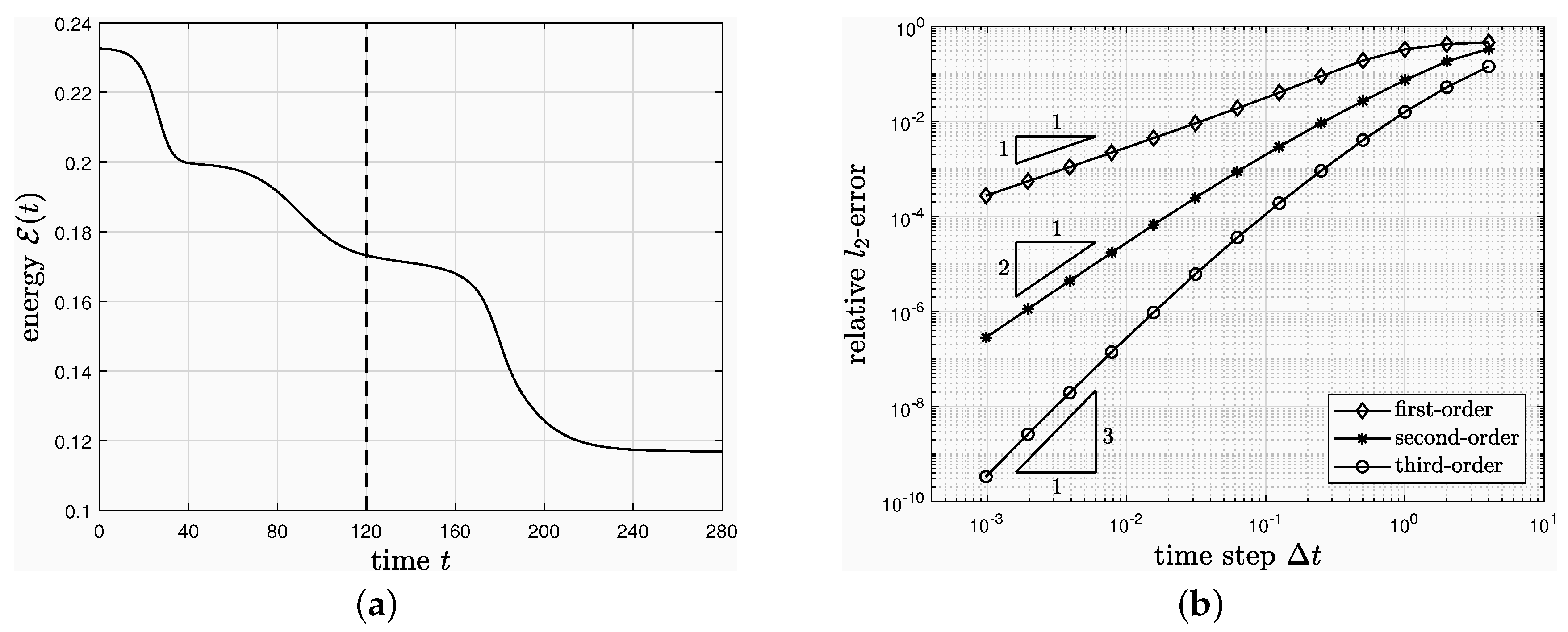
4.1. Convergence Test

We demonstrate the convergence of the proposed schemes with the initial conditions

$$\begin{array}{ccc}\hfill c_1(x,0)& =& \frac{1}{3}+0.01cos\frac{3}{2}x,c_2(x,0)=\frac{1}{3}+0.02cosx,\hfill \\ \hfill c_3(x,0)& =& 1-c_1(x,0)-c_2(x,0)\hfill \end{array}$$

on $\mathsf{\Omega }=[0,2\pi ]$. We set $ϵ=0.25$ and compute $\mathbf{c}(x,t)$ for $0<t\le 280$. The grid size is fixed to $h=2\pi /64$, which provides enough spatial accuracy. To estimate the convergence rate with respect to $\Delta t$, simulations are performed by varying $\Delta t=2^{-10},2^{-9},\dots ,2^2$. We take the quadruply over-resolved numerical solution using the third-order scheme as the reference solution. Figure 1a,b shows the evolution of $\mathcal{E}\left(t\right)$ for the reference solution and the relative $l_2$-errors of $\mathbf{c}(x,120)$ (this time is indicated by a dashed line in Figure 1a) for various time steps, respectively. It is observed that the schemes give desired order of accuracy in time.

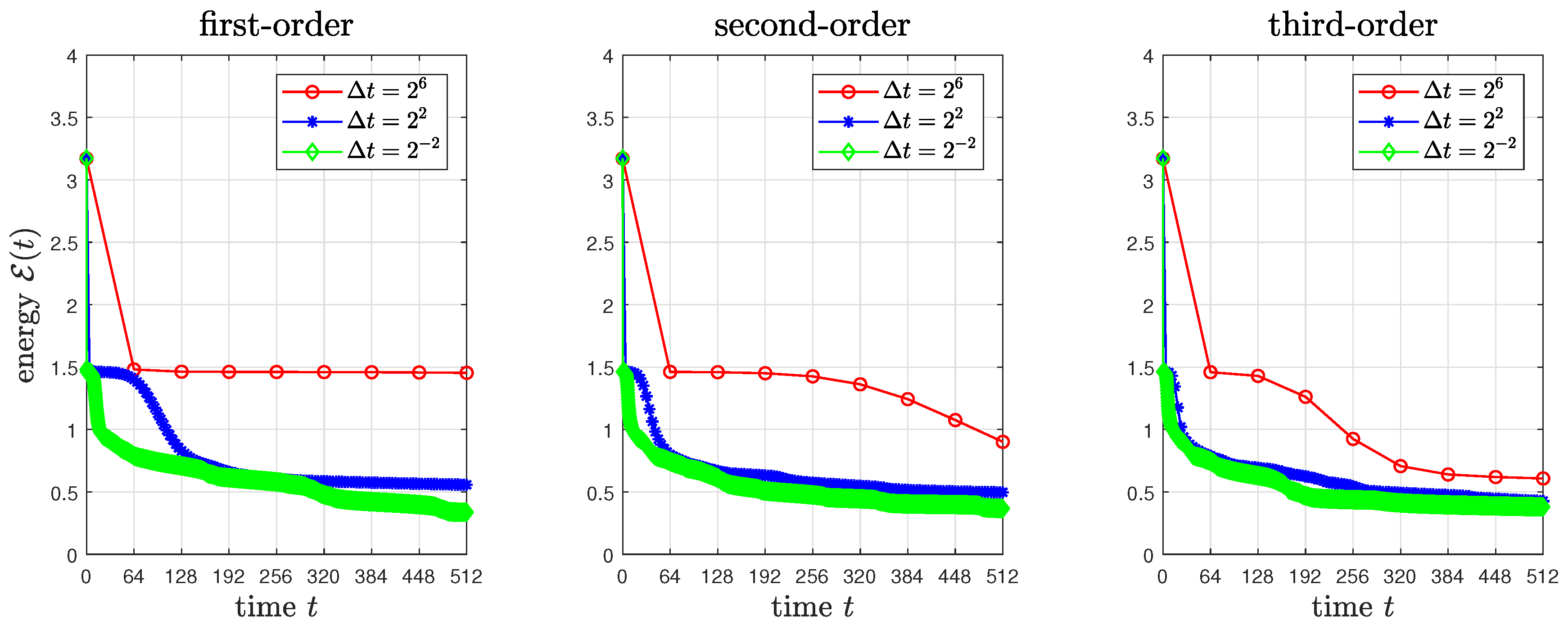
4.2. Energy Stability of the Proposed Schemes

To investigate the energy stability of the proposed schemes, we consider the phase separation of a ternary system with the initial conditions

$$\begin{array}{c}{c}_1(x,y,0)=\frac{1}{3}+\mathrm{rand}(x,y),c_2(x,y,0)=\frac{1}{3}+\mathrm{rand}(x,y),\hfill \\ c_3(x,y,0)=1-c_1(x,y,0)-c_2(x,y,0)\hfill \end{array}$$

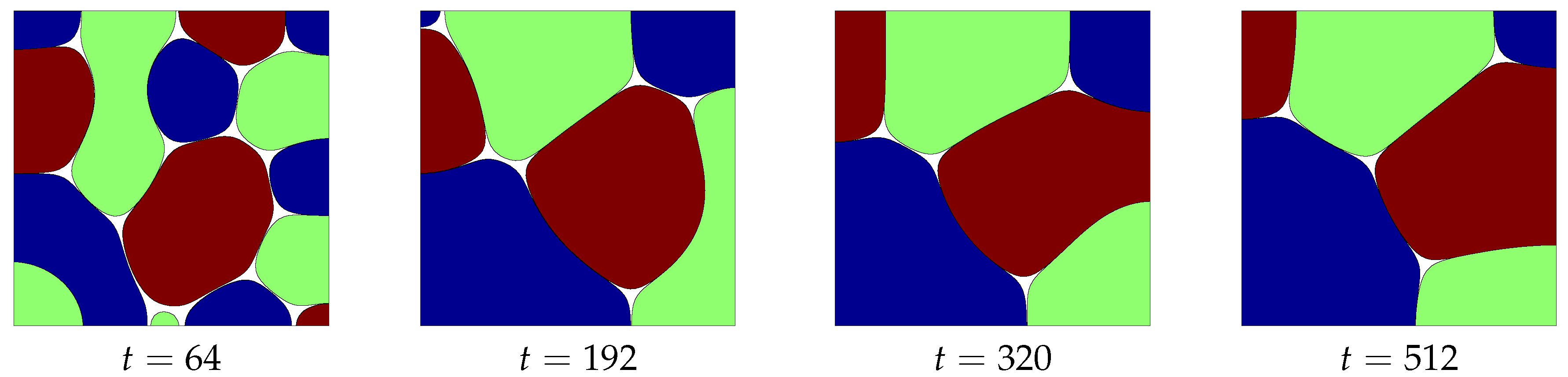
on $\mathsf{\Omega }=[0,2\pi ]\times [0,2\pi ]$. Here, $\mathrm{rand}(x,y)$ is a random number between $-0.1$ and $0.1$, and we use $ϵ=0.1$ and $h=2\pi /64$. Figure 2 shows the evolution of $\mathcal{E}\left(t\right)$ using the first-, second-, and third-order schemes with different time steps. All energy curves are nonincreasing in time even for sufficiently large time steps. Figure 3 shows the evolution of $\mathbf{c}(x,y,t)$ using the third-order scheme with $\Delta t=2^{-2}$.

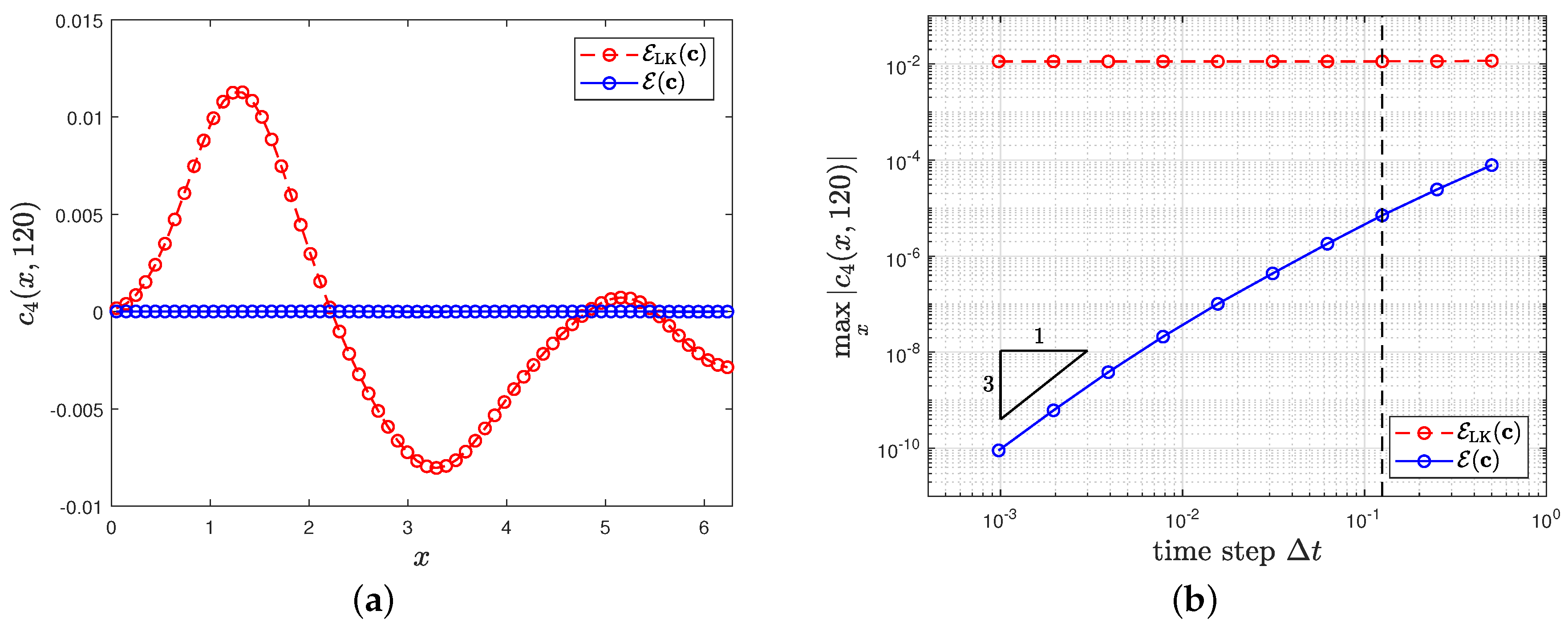
4.3. Consistency of Null-Phase

To confirm whether consistency of null-phase guarantees, we consider that only three phases are present but the simulation is performed using a quaternary system, i.e., we take the initial conditions as

$$\begin{array}{ccc}\hfill c_1(x,0)& =& \frac{1}{3}+0.01cos\frac{3}{2}x,c_2(x,0)=\frac{1}{3}+0.02cosx,\hfill \\ \hfill c_3(x,0)& =& 1-c_1(x,0)-c_2(x,0),c_4(x,0)=0\hfill \end{array}$$

on $\mathsf{\Omega }=[0,2\pi ]$. For ${\mathcal{E}}_{\mathrm{LK}}\left(\mathbf{c}\right)$, we employ the convex splitting in [17] and also apply the third-order scheme in Equation (10) with $\mathbf{R}$ in (14). We use $ϵ=0.25$, $h=2\pi /64$, and the third-order scheme and compute $\mathbf{c}(x,t)$ for $0<t\le 120$. Figure 4a,b shows $c_4(x,120)$ obtained with $\Delta t=2^{-3}$ and ${max}_x\left|c_4(x,120)\right|$ for various time steps, respectively, for two models ${\mathcal{E}}_{\mathrm{LK}}\left(\mathbf{c}\right)$ and $\mathcal{E}\left(\mathbf{c}\right)$. As shown in Figure 4, ${\mathcal{E}}_{\mathrm{LK}}\left(\mathbf{c}\right)$ generates $c_4$, even though the initial condition for $c_4$ is zero. We believe that this generation is not a result of numerical computation but a consequence of the model error not satisfying Criterion A. On the other hand, for $\mathcal{E}\left(\mathbf{c}\right)$, the maximum of $c_4$ is only controlled by the accuracy of the numerical scheme.

4.4. No Additional Phase Generation on Interface

To test whether spurious phase generation takes place on interfaces, we consider the phase separation of a quaternary system with the initial conditions

$$\begin{array}{cc}{c}_1(x,y,0)=\frac{1}{4}+\mathrm{rand}(x,y),\hfill & c_2(x,y,0)=\frac{1}{4}+\mathrm{rand}(x,y),\hfill \\ c_3(x,y,0)=\frac{1}{4}+\mathrm{rand}(x,y),\hfill & c_4(x,y,0)=1-{\sum }_{i=1}^3{c}_i(x,y,0)\hfill \end{array}$$

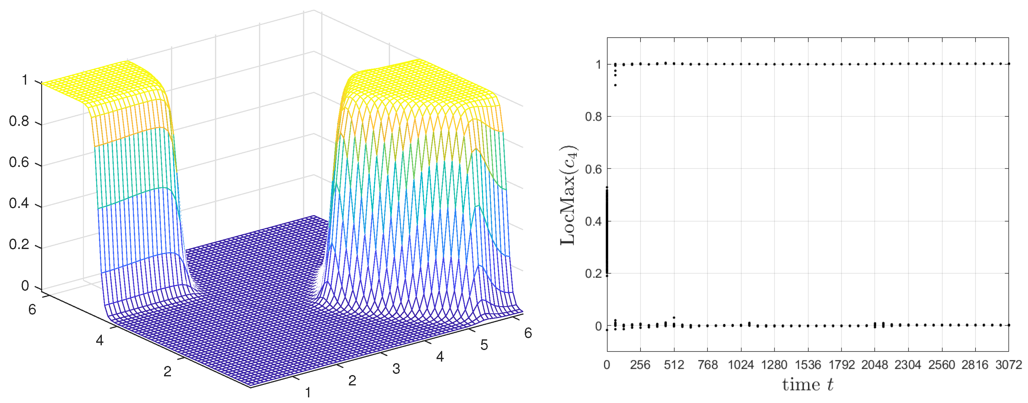
on $\mathsf{\Omega }=[0,2\pi ]\times [0,2\pi ]$. Here, $rand(x,y)$ is a random number between $-0.1$ and $0.1$. For ${\mathcal{E}}_{\mathrm{LK}}\left(\mathbf{c}\right)$, we employ the convex splitting in [17] and also apply the third-order scheme in Equation (10) with $\mathbf{R}$ in Equation (14). We use $ϵ=0.05$, $h=2\pi /64$, and $\Delta t=2^2$. Figure 5 and Figure 6 show $c_4(x,y,T=3072)$ and local maximum of $c_4(x,y,t)$ for $0\le t\le T$ using the third-order scheme for two models ${\mathcal{E}}_{\mathrm{LK}}\left(\mathbf{c}\right)$ and $\mathcal{E}\left(\mathbf{c}\right)$, respectively.

As shown in Figure 5, ${\mathcal{E}}_{\mathrm{LK}}\left(\mathbf{c}\right)$ generates spurious phase at two triple junction points where the first, second, and third components meet. On the other hand, $\mathcal{E}\left(\mathbf{c}\right)$ in Figure 6 suppresses the formation of spurious phases on interfaces almost completely. To quantify the spurious phase generation, we define $\mathrm{LocalMax}\left(c_i\right)$ at time t as a set of local maxima of $c_i(x,y,t)$ in $\mathsf{\Omega }$. We observe many local maxima near $0.25$ at the beginning of evolution but only two maxima 0 and 1 are expected for the fully separated phases. The model with $\mathcal{E}\left(\mathbf{c}\right)$ shown in Figure 6 gives well separated phases over time, whereas the model with ${\mathcal{E}}_{\mathrm{LK}}\left(\mathbf{c}\right)$ has another local maximum at about $0.043$ due to the spurious phases at the junction points. We believe that this spurious phases generation is not a result of numerical computation but a consequence of the model error not satisfying Criterion B.

5. Conclusions

In this paper, we consider the multi-component CH system where all phase variables are nonlinearly coupled. To study the dynamics of this system, we propose the high-order energy stable scheme based on the convex splitting idea. To handle the nonconvex, nonconcave term in the energy, we add an auxiliary term, which yields a convex–concave decomposition of the energy. We combine the convex splitting with the specially designed implicit–explicit RK method thus developed the high-order cCS scheme. We confirmed that the schemes give desired order of accuracy in time and are unconditionally energy stable. By using the scheme, we also demonstrated that the use of $\mathcal{E}\left(\mathbf{c}\right)$ is crucial and gives very significant qualitative improvement of the results compared to the additive model ${\mathcal{E}}_{\mathrm{LK}}\left(\mathbf{c}\right)$.