Blended Root Finding Algorithm Outperforms Bisection and Regula Falsi Algorithms


Computer Science Department, Missouri University of Science and Technology, Rolla, MO 65409, USA
Mathematics 2019, 7(11), 1118; https://doi.org/10.3390/math7111118
Submission received: 5 October 2019
/
Revised: 6 November 2019
/
Accepted: 11 November 2019
/
Published: 16 November 2019
(This article belongs to the Special Issue Numerical Modeling and Analysis)
Abstract
:Finding the roots of an equation is a fundamental problem in various fields, including numerical computing, social and physical sciences. Numerical techniques are used when an analytic solution is not available. There is not a single algorithm that works best for every function. We designed and implemented a new algorithm that is a dynamic blend of the bisection and regula falsi algorithms. The implementation results validate that the new algorithm outperforms both bisection and regula falsi algorithms. It is also observed that the new algorithm outperforms the secant algorithm and the Newton–Raphson algorithm because the new algorithm requires fewer computational iterations and is guaranteed to find a root. The theoretical and empirical evidence shows that the average computational complexity of the new algorithm is considerably less than that of the classical algorithms.
1. Introduction
Non-linear equations arise in most disciplines including computer science, natural sciences (civil engineering, electrical engineering, mechanical engineering), biological engineering and social sciences (psychology, economics), etc. Problems such as minimization, target shooting, orbital motion, plenary motion, etc., often lead to finding roots of non-linear functional equations [1,2,3,4,5,6].
There are classical root-finding algorithms: bisection, false position, Newton–Raphson, modified Newton–Raphson, secant and modified secant method, for finding roots of a non-linear equation f(x) = 0 [7,8,9,10,11]. From these algorithms, the developer has to explore and exploit the algorithm suitable under specified constraints on the function and the domain. Although some researchers have implemented genetic algorithms to find the roots of equations and compared the results with the results of classical algorithms [12], it is not the intent of this paper to go into that area. Finding the roots of an equation is a fundamental problem in engineering fields. Every book on numerical methods has details of these methods and recently, papers are making differing claims on their performance [13,14]. There is not a single algorithm that works best for every function. We present a new blended algorithm that outperforms all the existing algorithms. See Section 4 for experimental data validating the performance of the new algorithm.
Most optimization problems lead to solving equations for the value of an optimizing parameter, hence determining the root of a related equation. Sometimes, in applications, we may need to determine when will two functions g(x) and h(x) be equal, i.e., g(x) = h(x). This translates into finding roots of the classical equation f(x) = g(x) − h(x) = 0. Similarly, the optimal value of g(x) can be determined by a root of the equation = 0, which implies an equation = f(x) = 0. Numerical techniques are used when an analytic solution is not available, see Section 2.
Thus, a root-finding algorithm implies solving an equation defined by a function. Some root-finding algorithms do not guarantee that they will find a root. If such an algorithm does not find a root, that does not mean that no root exists. Even though classical methods have been developed and used for decades, enhancements are progressively made to improve the performance of these methods. No single classical method outperforms another method on all functions [15,16]. A method may outperform other methods on one dataset, and may produce inferior results on another dataset. Different methods have different strengths/weaknesses. A dynamic new blended algorithm (blend of bisection and false position) is presented here by taking advantage of the best in bisection and false position methods to locate the roots. Its computational efficiency is validated by empirical evidence by comparing it with the existing methods. The new blended algorithm is a tested technique that outperforms other existing methods by curtailing the number of iterations required for approximations (Table 1), while retaining the accuracy of the approximate root. Table 2 is a listing of functions from literature used to test the validity of results.
This paper is organized as follows. Section 2 is a brief description of the classical methods bisection, regula falsi, Newton–Raphson, secant; their strengths and pitfalls. Section 3 describes the new blended algorithm. Section 4 gives a theoretical justification for the blended algorithm. Section 5 presents experimental results validating the performance of the new algorithm. Section 6 is the conclusion.
2. Background
There are four classical methods for finding roots of non-linear equations: bisection, false position, Newton–Raphson and secant. For completeness, we briefly clarify methods for (1) root approximation, (2) error calculation and (3) termination criteria. Since there is no single optimal algorithm for root approximation, we will provide a new blended algorithm that outperforms bisection and regula falsi methods. Normally, when faced with competing choices, the simplest is the accurate one.
We restrain this discussion to finding a single root instead of all the roots of an equation. In case an equation has several roots, we can delineate an interval where the desired root is to be found.
2.1. Bisection Method
The bisection method is (1) based on binary chopping of irrelevant subintervals, (2) a virtual binary search, and (3) guaranteed to converge to the root, see Algorithm 1. The bisection method is static, the length of the subinterval at each iteration is independent of the real-valued function and R denotes the set of all real numbers. No matter what the function is, the root-error upper bound is fixed at each iteration and can be determined a priori. By specifying the root-error tolerance, the upper bound on the number of iterations can be predetermined quickly.
Problem If a function f:[a, b] → R, is such that (1) f(x) is continuous, (2) R is the set of all real numbers and (3) f(a) and f(b) are of opposite signs, i.e., f(a)·f(b) < 0, then there exists a root r ∈ [a, b] such that f(r) = 0.
| Algorithm 1: Bisection Method |
| 1. Input: f and [a, b], ∈, maxIterations |
| 2. Output: root r, bracketing interval [ak, bk] |
| 3. //initialize |
| 4. k = 1; [ak, bk] = [a, b] |
| 5. repeat |
| 6. //compute the mid-point |
| 7. |
| 8. if f(ak)·f(rk) < 0, |
| 9. ak+1 = ak; bk+1 = rk |
| 10. elseif f(rk)·f(b1) < 0, |
| 11. ak+1 = rk; bk+1 = bk |
| 12. endif |
| 13. r = rk |
| 14. k = k+1; |
| 15. until |f(r)| < ∈ or k > maxIterations |
The algorithm proceeds using [a1, b1] = [a, b] as the initial interval of continuity of f. The first approximate root is
, the middle point of the interval [a1, b1]. The actual root lies in the interval [a1, r1] or [r1, b1]. If f(r1) = 0, r1 is the root. If f(a1) and f(r1) are of opposite sign, then f(a1)·f(r1) < 0, and the true root lies in [a1,r1]. If f(r1) and f(b1) are of opposite sign, then f(r1)·f(b1) < 0, and the true root lies in [r1,b1]. The new interval is denoted by [a2, b2]. At each iteration, the new root and next root bracketing sub-interval is generated. In general, for each iteration k, the approximation is the middle point of [ak, bk], if f(ak)·f(rk) < 0, the root lies in [ak, rk] else if f(rk)·f(bk) < 0, the root lies in [rk, bk] or rk is the root. Then the next interval is denoted by [ak+1, bk+1] where rk is one of its endpoints. The iterations continue until the termination criteria are satisfied.
2.1.1. Advantages of the Bisection Method
Since the method brackets the root, at each iteration the length of the root-bracketing interval is halved. Thus, the method guarantees the decline in error in the approximate solution at each iteration. The convergence of the bisection method is certain because it is simply based on halving the length of the bracketing interval containing the root.
2.1.2. Drawbacks of the Bisection Method
Though the convergence of the bisection method is guaranteed, its rate of convergence is slow, and as such it is quite difficult to extend to use for systems of equations. If for any iteration, root approximation is very close to an endpoint of bracketing interval, bisection does not take advantage of this information, it will take some pre-determined number of iterations to reach the root [7].
2.2. False Position (Regula Falsi) Method
The motivation for innovative methods arises from the poor performance of the bisection method. The false position method is known by various names, for example, the double false position, regula falsi or linear interpolation. It is a very old method for solving equations in one unknown. This method differs from bisection in the way the estimates are calculated. The false position is a dynamic method; it takes advantage of the location of the root to make a conceivably better appropriate selection. Unfortunately, this method does not perform as well as expected, for all functions, see Figure 1, Figure 2, Figure 3 and Figure 4.
Here also, the function f:[a, b] → R is such that (1) f(x) is continuous, (2) R is the set of all real numbers and (3) f(a) and f(b) are of opposite signs, i.e., f(a)·f(b) < 0. The algorithm uses a, b as the two initial estimates of the root. The false position method uses both endpoints as two starting values ro = a, r1 = b. The secant line through points (r0, f(r0)) and (r1, f(r1)) intersects the x-axis to yield the next estimate, r2. For successive estimates, the false position method intersects the secant line through (rn−1, f(rn−1)) and (rn−2, f(rn−2)) with the x-axis for the approximation, rn,
for n ≥ 2.
The approximations, rn, are ensured to be bracketed as in the case of bisection method. And one should note that the length of the brackets do not necessarily tend to zero. The pseudo-code of the Algorithm 2 is as follows.
| Algorithm 2: False Position Method |
| 1. Input: f and [a, b], ∈, maxIterations |
| 2. Output: root r, bracketing interval [ak, bk] |
| 3. //initialize |
| 4. r0 = a; r1 = b |
| 5. k = 1; [ak, bk] = [a, b] |
| 6. repeat |
| 7. //compute the secant line -point |
| 8. rk = ak − |
| 9. if f(ak)·f(rk) < 0, |
| 10. ak+1 = ak; bk+1 = rk |
| 11. elseif f(rk)·f(b1) < 0, |
| 12. ak+1 = rk; bk+1 = bk |
| 13. endif |
| 14. r = rk |
| 15. k = k+1; |
| 16. until |f(r)| < ∈ or k > maxIterations |
2.2.1. Justification
The root approximation error calculation in the bisection method is straight forward (see Section 4); in each iteration root approximation error is halved, i.e., root approximation error in the n-th step is no more than . This is not the case for the false position method. If a is sufficiently close to the root r, then f(a) is close to f(r) due to continuity of f. Then the slope of the secant line, , is approximately equal to . The closer b is to r, the closer the secant line is to tangent, f′(r), though, it is not required that f be differentiable. Since = , the slope of secant line, it becomes the slope of the tangent line slope as b becomes a or r. The closer the secant line is to the tangent line, the faster the convergence of iterations [17], because the Newton method is faster than the secant method.
In Section 3, we present a dynamic algorithm blend of bisection and false position methods.
2.2.2. Advantages of the False Position Method
It is guaranteed to converge due to the decreasing length of the root-bracketing interval. It is fast when you know the linear nature of the function.
2.2.3. Drawbacks of the False Position Method
For the false position method, there is no way to determine a priori the number of iterations needed for convergence. And one should note that the length of the brackets does not necessarily tend to zero. If we cannot ensure that the function can be interpolated by a linear function, then applying the false position method can result in worse results than the bisection method. The problem occurs when the function is convex, concave up or concave down. According to [18], for a concave down function, the left endpoint remains stationary and the right endpoint updates in each iteration. For concave up function, the right endpoint remains stationary and the left endpoint updates in each iteration. This is not an accurate statement, it works for some of the functions, not all the functions. Figure 1, Figure 2, Figure 3 and Figure 4 contradict their statement. It depends on the convexity of the function, not concavity up or down. When the root is very close to the endpoints of the interval, the convergence of the sequence of approximations can become extremely slow.
In the example in Figure 1, Figure 2, Figure 3 and Figure 4, four functions are used with the same tolerance and 10 as the upper limit of the number of iterations for display purposes. The purpose is to show how the algorithm works for the false position method. In the interest of simplicity of plots, algorithms terminate before reaching the error-tolerance.
2.3. Newton–Raphson Method
Newton–Raphson is also called a fixed-point iteration method. This method requires that the function be differentiable. If the function f(x) is differentiable on the domain of the function, and r0 is the initial guess, then the first approximation r1 is obtained by intersection of the tangent at (r0, f(r0)) with the x-axis, and is defined by
and successive approximations are
for n ≥ 2.
This method converges provided |g′(x)| < 1 where g(x) = x − for x in the domain of f(x). For functions where there is a singularity such that it reverses sign at the singularity, the Newton–Raphson method may converge on the singularity.
2.3.1. Advantages of the Newton–Raphson Method
The convergence rate is linear, and this method is very fast as compared to the bisection and false position methods. If f(k)(x) = 0 for integers k < m, then m is the multiplicity of the root. If we know the multiplicity, m, of the root, it can be further improved with faster convergence to the root [7]. The updated iteration formula becomes,
for n ≥ 1.
2.3.2. Disadvantages of the Newton–Raphson Method
The only pitfall is that it fails if the derivative, f′(x), is near zero at some iteration. For example, Newton–Raphson method fails to compute r1 for f(x) = x2 − 1 where r0 = 0. But it does not create a problem in some cases where the singularity in f’(x) cancels with f(x). For example, f(x) = x3 with r0 = 0 does result in r1 = 0.
2.4. Secant Method, Modified Secant Method
The secant method requires that the function be differentiable. When it is not easy to compute the derivative of the function, the secant method approximates the derivative with the slope of a secant line. Thus, in the absence of a derivative of the function, the secant method is a modification of the Newton–Raphson method. It does not need differentiability as well as bracketing. The false position method ensures that approximations are bracketed, and the secant method simply uses the last two values to approximate the tangent. Thus, the secant method is not guaranteed to converge.
The convergence rate of the secant method is super linear. Thus, the convergence rate is between that of the bisection method and the Newton–Raphson’s method. The secant method requires two initial values, whereas Newton–Raphson requires only one starting value. If the function f(x) is differentiable, and r0, r1 are two initial guesses, then the approximations of the secant method can be written as
for n ≥ 2.
If the secant line is closer to the tangent line, we can get a better estimate. The closer the points defining the secant line, the better the approximation of the secant line is to the tangent line. To accomplish this improvement, we replace rn−2 by a value even closer to rn−1. Thus, for a better estimate of the slope of the secant line, we can define a small positive constant, , so that it replaces rn−2 with rn−1 − δ (or even rn−1 δ before computing the next iteration as
or
The success of this method will depend on the choice of sufficiently small real positive . For practical reasons, we choose positive δ, such that 0 < < ||.
Advantages and Shortcomings
It has the advantage of finding a bracketing-interval quickly, but the choice of delta must be made adaptively, otherwise, the algorithm runs the risk of missing the root.
Some researchers, experimented on f(x) = x − cos(x) on a closed interval [0,1] and concluded that the secant method is better than the bisection and Newton–Raphson methods [12,19]. It is not accurate to make a conclusion from one function. We show that this statement is not accurate, see Table 3, Table 4, Table 5, Table 6 and Table 7.
2.5. Genetic Algorithms and Swarm Intelligence
Genetic algorithm design and swarm intelligence is not the purpose of this paper, but for completeness, we make a passing reference to what some researchers have found. The genetic algorithm is based on the concept of chromosomes population, genotype, phenotype, objective function and fitness values. MATLAB has built-in functions ga for implementing genetic algorithms, and gatool for user friendly GUI interactive experiments. Genetic algorithms are a wide field on its own, and we will not spend much time on this except to comment how the new algorithm compares with the genetic algorithm findings by other researchers [12].
Several researchers including [12,16,19] have attempted to use the genetic algorithm to compare with the classical methods. They have conflicting experiences, probably depending on the function and constraints they use. Moazzam et al. [16] solved the transcendental equation x2 − x − 2 = 0 by the genetic algorithm as well as the bisection and false position methods. The bisection, false position and genetic algorithms take 21, 17 and 7 iterations in Microsoft Visual C++, respectively. They announced that the genetic algorithm is better than classical methods. We find that the new blended algorithm (blend of the bisection and false position methods) outperforms all their findings [12]. Nayak et al. [19] implemented the genetic algorithm on f(x) = x2 + 2x − 7, and Sirinivasa et al. [12] experimented on f(x) = x2. They made no comparison of genetic results with classical algorithms.
Swarm intelligence is another idea of coordinating massive numbers of individual technology entities to work together. This kind of nature-inspired artificial intelligence resulting from the swarm principles can offer insights to help humans solve complicated real-world problems. Swarm intelligence (SI) optimization algorithms have attracted significant attention due to their ability to solve complex optimization problems. The underlying idea behind all SI algorithms is similar, and various SI algorithms differ in their details. They are beyond the scope of this paper, but worth exploring. We will explore genetic algorithms, swarm intelligence and statistical analysis for solving related engineering problems in a future project.
2.6. Effectiveness and Efficacy of Root Approximation Iterations
2.6.1. Methods for Root-Error Calculation for Termination Criterion
There are various ways to measure error when approximating a root of an equation at successive iterations to continue to a more accurate approximate root. To determine rn for which f(rn) 0, we proceed to analyze as follows.
The iterated root approximation error can be
or
AbsoluteRootError = |rn − rn−1|
Since a root can be zero, in order to avoid division by small numbers, it is preferable to use absolute error |rn − rn−1| for convergence testing. Another reason is that if rn = 2−n, then is always 1. It can never be less than 1, so the relative root-error tolerance does not work on all functions.
Since the function value is expected to be zero at the root, an alternate, cognitively more appealing error test, is to use |f(rn)| for error consideration. There are three versions of this concept. They are
or
or
for comparison criteria. Since f(rn) is to be close to zero, in order to avoid division by small numbers, we discard using and since |f(rn−1) − f(rn)| can be close to zero without |f(rn)| being close to zero, we discard using |f(rn−1) − f(rn)| in favor of using only |f(rn)|, trueValue error. For example, f(rn) = (n−1)/n is such an example. To avoid using the latter two criteria for this reason, we exploit the first one, |f(rn)|.
TrueValueError = |f(rn)|
AbsoluteValueError = |f(rn−1) − f(rn)|
Now we are left with two options for error analysis |rn − rn−1| and |f(rn). Since rn and rn−1 can be closer to each other without f(rn) being closer to zero, between the options |rn − rn−1| and |f(rn)|, we find that |f(rn)|is the only reliable metric for analyzing approximation error because we can have a sequence {rn} where |rn − rn−1| goes to zero, but |f(rn)| does not go to zero. For example, if rn = 1 + 1/n, and f(rn) = rn, then |rn − rn−1| → 0, but |f(rn)| → 1. This example justifies reasoning. Hence, we use this criterion for error analysis for all the methods uniformly in order to circumvent pathological cases.
2.6.2. Stopping Criteria for Halting Condition
Stopping criteria plays a major role in simulations. We start with an initial guess(es), and by iteratively applying the selected criteria, we get a sequence of root values of an increasingly accurate estimation of the root, hopefully, converging to a real root. The tradeoff between accuracy and efficiency is the accuracy of the outcome. In order to obtain n significant digit accuracy [7], let ∈s be the stopping error and let ∈a be the approximation error at any iteration. If ∈a < ∈s the algorithm stops iterating. With ∈s = 5/10n−1, we have n significant digit accuracy in the outcome. In pathological cases, ∈a may never be useful and we have to specify upper bound on the number of iterations. We use both the error tolerance and iteration bound. The program terminates whichever is satisfied first.
3. Blended Algorithm
Instead of brute force application of the bisection or false position method solely, we selectively apply the most relevant method at each step to redefine the approximate root and bracketing interval. Thus, we construct a new blended algorithm, Algorithm 3, that outperforms the bisection and false position methods. It also outperforms the Newton–Raphson and secant methods (Table 3, Table 4, Table 5, Table 6 and Table 7) as long as the f(a)·f(b) < 0 is determined. At each iteration, the root estimate is computed with both bisection and false position methods, and the hybrid of the two is selected for the next approximation. This prevents the unnecessary iterations performed in either method (see Table 1 column 2). This method does not require differentiability of the function as required by Newton–Raphson and secant methods. The blended algorithm outperforms them when f(a)·f(b) < 0.
| Algorithm 3: Blended Bisection and False Position |
| 1. Input: f and [a, b], ∈, maxIterations |
| 2. Output: root r, bracketing interval [ak+1, bk+1] |
| 3. //initialize |
| 4. k = 0; a1 = a, b1 = b |
| 5. repeat |
| 6. //compute the mid point |
| 7. mk = , and ∈m = |f(mk)| |
| 8. //compute the secant line point, |
| 9. sk = ak − and ∈s = |f(sk)| |
| 10. if |f(mk)| < |f(sk)|, |
| 11. // f(mk) is closer to zero, Bisection method determines bracketing interval [bak+1, bbk+1] |
| 12. rk = mk |
| 13. ∈a = ∈m |
| 14. if f(ak)·f(rk) < 0, |
| 15. bak+1 = ak; bbk+1 = rk |
| 16. else |
| 17. bak+1 = rk; bbk+1 = bk |
| 18. endif |
| 19. else |
| 20. // f(sk) is closer to zero, False Position method determines bracketing interval [fak+1, fbk+1] |
| 21. rk = sk |
| 22. ∈a = ∈s |
| 23. if f(ak)·f(rk) < 0, |
| 24. fak+1 = ak; fbk+1 = rk |
| 25. else |
| 26. fak+1 = rk; fbk+1 = bk |
| 27. endif |
| 28. //Since the root is bracketed by both [bak+1, bbk+1] and [fak+1, fbk+1] |
| 29. [ak+1, bk+1] = [bak+1, bbk+1] ∩ [fak+1, fbk+1] |
| 30. // outcome: iteration complexity, root, and error of approximation |
| 31. iterationCount = k |
| 32. r = rk |
| 33. error = ∈a = |f(r)| |
| 34. k = k + 1 |
| 35. until |f(r)| < ∈ or k > maxIterations |
4. Complexity Issue
The new algorithm is a blend of the bisection and false position algorithms. The number of iterations to find a root depends on the criteria used to determine the root accuracy. If f(x) is used, then complexity depends on the function as well as the method. If relative error is used, it does not work for every function, as seen in Section 2.6. Most of the time, absolute error, ∈, is used as the stopping criteria. For functions on interval [a, b] with the bisection method, the upper bound nb(∈) on the number of iterations can be predetermined from < ∈ and is lg ((b − a)/∈). For the false position method, it depends on the convexity and location of the root near the endpoint of the bracketing interval. The bound nf(∈) for the number of iterations for the false position method cannot be predetermined, it can be less, nf(∈) < nb(∈) = lg ((b − a)/∈) (see Table 1) or can be greater, nf(∈) > nb(∈) = lg ((b − a)/∈) (see Figure 1, Figure 2, Figure 3 and Figure 4). The complexity of the genetic algorithm was found to be close to the false position algorithm [16]. The number of iterations, n(∈), in the new algorithm is less than min(nf(∈), nb(∈)). This is confirmed from the algorithm and is validated with the empirical computations in Section 5. Newton–Raphson and secant methods have quadratic convergence, but are not guaranteed to converge unless additional constraints are imposed on the functions.
5. Discussions
Many researchers focused their attention toward using such methods to solve their problems. The roots are calculated, along with the number of iterations within a specified tolerance. All the existing methods are compared. Error analysis is performed. It is determined that the blended algorithm (blend of bisection and false position) outperforms the other algorithms.
5.1. Empirical Testing Evidence
We have tested our new algorithm against other methods on examples used in the literature (Table 2) and validated that the new algorithm outperforms these methods. We have not included the genetic algorithm testing here, but our tests compare with previously announced results to show it outperforms the genetic algorithm as well (Table 1).
5.2. Experiments Using MATLAB
Moaazzam used Microsoft Visual C++ to find roots [16]. We used MATLAB R2018b64bit on MacMojave2.2GHz16GB. For validation purposes, we used the same quadratic equation for root of x2 − x − 2 = 0 on interval [1,4]. To find a root of this equation, the bisection method made 19 iterations to find a root value 2 and the false position method made 15 iterations (see Table 1). The genetic algorithm [16] made 6 iterations while our new improved algorithm made 2 iterations. They did not compare the genetic algorithm with secant or Newton–Raphson. The genetic algorithm was no better than the Newton–Raphson method. Interestingly, Ehiwario [19] compared bisection, Newton–Raphson and secant method, and claimed the secant method was better. That is also false as Table 1 shows that among the classical and genetic algorithms, Newton–Raphson outperforms them. Overall, the experiments have validated that the new algorithm outperforms all the classical algorithms in terms of the number of iterations required to find a root. Table 2 is a listing of (1) functions, (2) the domain of the function and (3) referenced authors who experimented with these functions. We tested the new algorithm on all of these functions and demonstrated the improvement by the algorithm by using the most cited function in the references.
Though the root approximation is almost the same in all methods, as expected, yet the number of iterations used to reach the root shows the improvement by the new algorithm. Table 1 is a description of the results of all the algorithms comparing the number of iterations used by each algorithm, the approximate root within those iterations, the root error and the bracketing interval of the approximate root for x2 − x − 2 = 0. Table 1 is a summary of the actual implementations of all these algorithms with the name of method, number of iterations performed, approximate root, error and bracketing interval containing the root. Table 3, Table 4, Table 5, Table 6 and Table 7 are detailed MATLAB output tables to support Table 2. Since it is hard to interpret the numbers in the tables of the algorithm outputs, graph plots are a preferred way to visualize the algorithm behavior. The plots of the execution of the algorithms are given in Figure 5, Figure 6, Figure 7, Figure 8 and Figure 9. The iterations column shows that the new blended algorithm is faster than other algorithms.
6. Conclusions
We have designed and implemented a new algorithm, a dynamic blend of the bisection and regula falsi methods. The algorithm was implemented in MATLAB R2018B 64 bit (maci64) on a MacBook Pro MacOS Mojave2.2GHz intel Core i716 GB2400MHz DDR4 Radeon Pro555X 4 GB. The count of iterations required to determine the root clearly shows the improvement of the new algorithm (Table 2). However, as desired and expected, the root approximation is almost the same in all algorithms. The implementation validates that the new algorithm outperforms in terms of number of computation iterations in both the bisection and false position algorithms all the time by a considerable margin. It is also observed that the new algorithm outperforms secant method and Newton–Raphson method (Table 1).
The algorithm was tested on all functions cited in Table 1. These functions were used by other researchers listed in the references. The most cited example was selected in the paper for comparison purposes. The results validate that the blended algorithm is effective both conceptually and computationally.
We find that some researchers have also used genetic algorithms. In this paper, we observed that the new algorithm uses fewer iterations than their findings on genetic algorithms. In the future, for better treatment of genetic algorithms as they pertain to root finding, we will develop our own genetic algorithms, as the blended algorithm over the bisection and false position methods presented in this paper.
Swarm intelligence is another idea of coordinating massive numbers of individual technology entities to work together. This kind of nature-inspired artificial intelligence resulting from the swarm principles can offer insights to help humans to solve complicated real-world problems. The underlying idea behind all SI algorithms is similar, and various SI algorithms differ in their details. We will explore genetic algorithms, swarm intelligence and statistical analysis for solving related engineering problems in a future project.
Funding
This research received no external funding.
Acknowledgments
The help from Clayton Price (teaching at the Missouri University of Science and Technology) for editing is sincerely and greatly appreciated. We also thank the referees for suggestions to improve the presentation of this paper.
Conflicts of Interest
The author declares no conflict of interest.
References
- Datta, B.N. Lecture Notes on Numerical Solution of Root Finding Problems. 2012. Available online: www.math.niu.edu/~dattab (accessed on 15 January 2019).
- Calhoun, D. Available online: https://math.boisestate.edu/~calhoun/teaching/matlab-tutorials/lab_16/html/lab_16.html (accessed on 13 June 2019).
- Thinzar, C.; Aye, N. Detection the storm movement by sub pixel registration approach of Newton Raphson method. Int. J. E Educ. E Bus. E Manag. E Learn. 2014, 4, 28–31. [Google Scholar]
- Ali, A.J.M. The application of numerical approximation methods upon digital images. Am. J. Signal Process. 2017, 7, 39–43. [Google Scholar] [CrossRef]
- Bruck, H.A.; McNeill, S.R.; Sutton, M.A.; Peters, W.H. Digital image correlation using Newton-Raphson method of partial differential correction. Exp. Mech. 1989, 29, 261–267. [Google Scholar] [CrossRef]
- Cofaru, C.; Philips, W.; van Paepegem, W. Pixel-level robust digital image correlation. Opt. Express 2013, 21, 29979–29999. [Google Scholar] [CrossRef] [PubMed]
- Chapra, S.C.; Canale, R.P. Numerical Methods for Engineers, 7th ed.; McGraw-Hill Publishers: Boston, MA, USA, 2015. [Google Scholar]
- Autar, K.K.; Egwu, E. Numerical Methods with Applications. 2008. Available online: http://www.numericalmethods.eng.usf.edu (accessed on 20 February 2019).
- Wolfram Mathematica. Available online: http://www.efunda.com/math/num_rootfinding-cfm (accessed on 15 February 2014).
- Charles, A.; Cooper, W.W. Non-linear power of adjacent extreme points methods in linear programming. Econometrica 2008, 25, 132–153. [Google Scholar] [CrossRef]
- Young, H.D.; Freedman, R.A. University Physics with Modern Physics, 11th ed.; Addison Wesley: Boston, MA, USA, 2004. [Google Scholar]
- Srivastava, R.B.; Srivastava, S. Comparison of numerical rate of convergence of bisection, Newton and secant methods. J. Chem. Biol. Phys. Sci. 2011, 2, 472–479. [Google Scholar]
- Iwetan, C.N.; Fuwape, I.A.; Olajide, M.S.; Adenodi, R.A. Comparative study of the bisection and Newton methods in solving for zero and extremes of a single-variable function. J. NAMP 2012, 21, 173–176. [Google Scholar]
- Ehiwario, J.C.; Aghamie, S.O. Comparative study of bisection, Newton-Raphson and secant methods of root-finding problems. IOSR J. Eng. 2014, 4, 2278–8719. [Google Scholar]
- Sivanandam, S.; Deepa, S. Genetic algorithm implementation using matlab. In Introduction to Genetic Algorithms; Springer: Berlin/Heidelberg, Germany, 2008; pp. 211–262. [Google Scholar] [CrossRef]
- Moazzam, G.; Chakraborty, A.; Bhuiyan, A. A robust method for solving transcendental equations. Int. J. Comput. Sci. Issues 2012, 9, 413–419. [Google Scholar]
- Harder, D.W. Numerical Analysis for Engineering. Available online: https://ece.uwaterloo.ca/~dwharder/NumericalAnalysis/10RootFinding/falseposition/ (accessed on 11 June 2019).
- Mathews, J.H.; Fink, K.D. Numerical Methods Using Matlab, 4th ed.; Prentice-Hall Inc.: Upper Saddle River, NJ, USA, 2004; ISBN 0-13-065248-2. [Google Scholar]
- Nayak, T.; Dash, T. Solution to quadratic equation using genetic algorithm. In Proceedings of the National Conference on AIRES-2012, Vishakhapatnam, India, 29–30 June 2012. [Google Scholar]
Figure 1.
Convex function concave up, right endpoint fixed.

Figure 2.
Convex function concave up, left endpoint fixed.

Figure 3.
Convex function concave down, right endpoint fixed.

Figure 4.
Convex function concave down, left endpoint fixed.

Figure 5.
Plot of blended algorithm execution.

Figure 6.
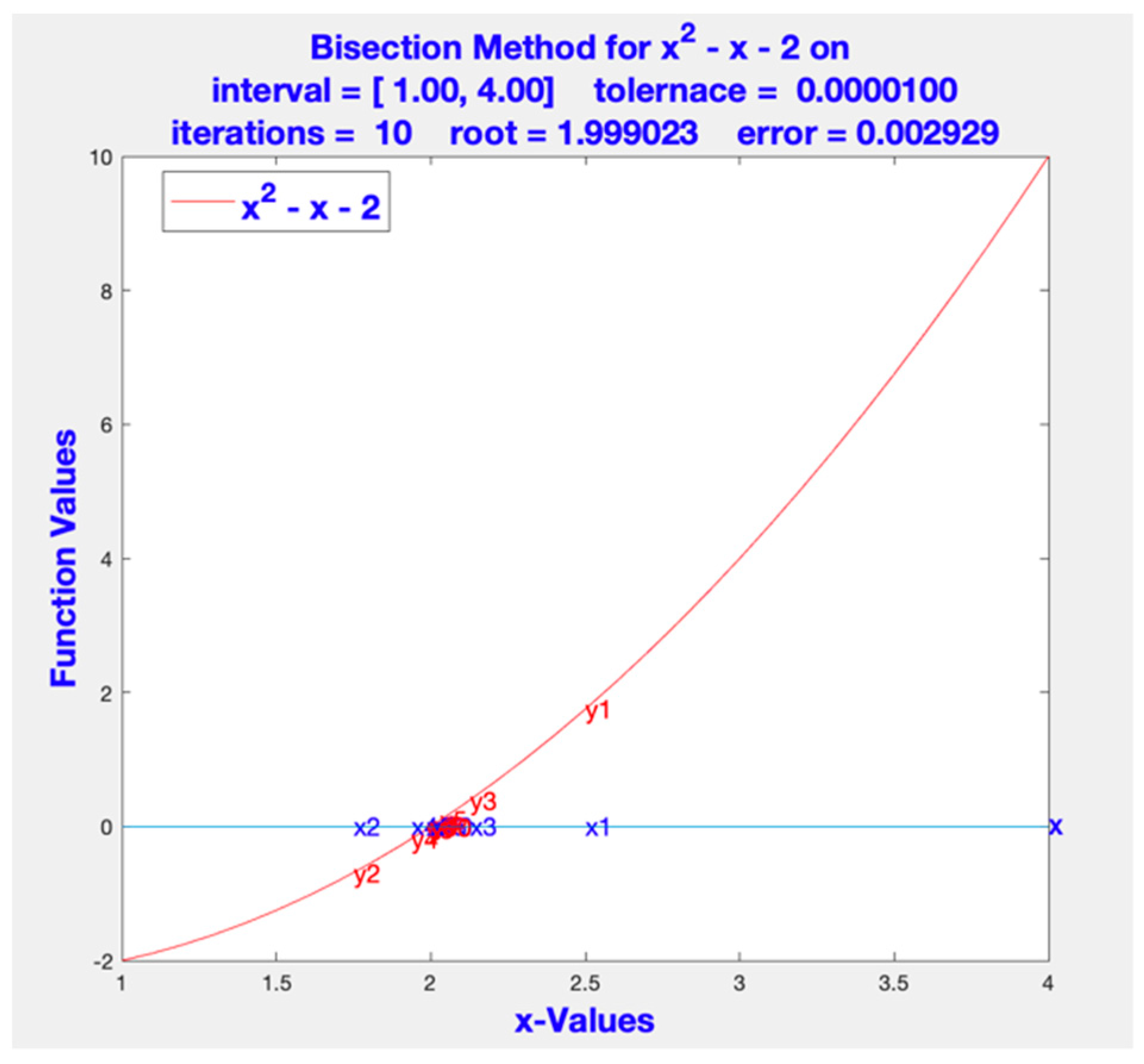
Plot of bisection algorithm execution.

Figure 7.
Plot of false position algorithm execution.

Figure 8.
Plot of Newton–Raphson algorithm execution.

Figure 9.
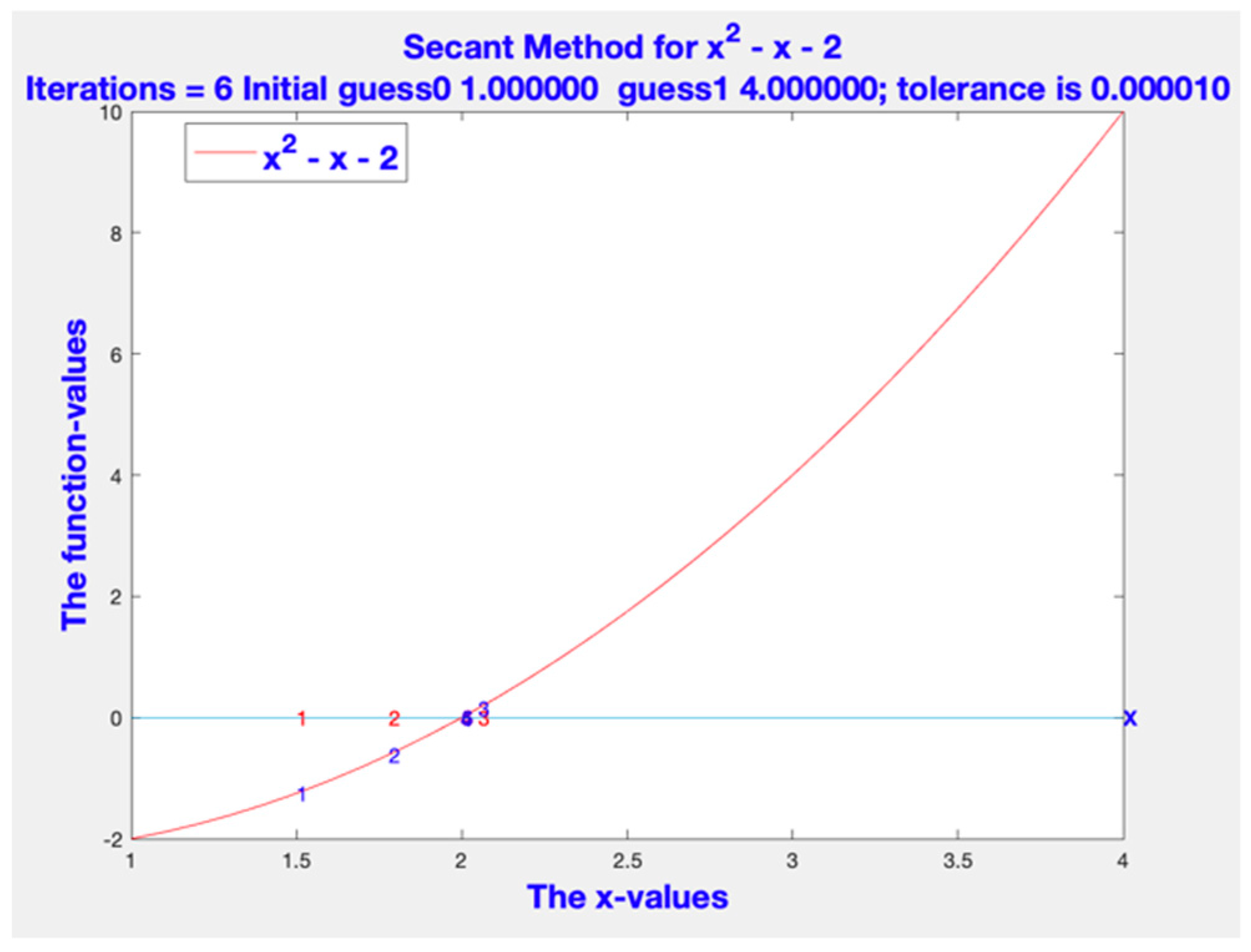
Plot of secant algorithm execution.


Table 1.
Comparison of classical algorithms iterations, AppRoot, error and interval bounds.
| Method | Iterations | AppRoot | Error | LowerB | UpperB |
|---|---|---|---|---|---|
| Bisection | 19 | 2.0000019 | 0.0000057 | 1.999996 | 2.000002 |
| FalsePosititon | 15 | 1.9999984 | 0.0000048 | 1.999998 | 4 |
| Secant | 6 | 2.0000001 | 0 | na | na |
| NewtonRaphson | 5 | 2 | 0 | na | na |
| Hybrid | 2 | 2 | 0 | 1.916667 | 2.05 |
Table 2.
From the literature function, domain interval and author of the function.
| Defining Function | Interval | Reference |
|---|---|---|
| x2 − 3 | [1, 2] | Harder |
| x2 − 5 | [2, 7] | Srivastava |
| x2 − 10 | [3, 4] | Harder |
| x2 − x − 2 | [1, 4] | Moazzam |
| x2 + 2x − 7 | [1, 3] | Nayak |
| x2 + 5x + 2 | [−6, 0] | Sivanandam |
| x3 − 2 | [0, 2] | Harder |
| xex − 7 | [−1, 1] | Calhun |
| x − cosx | [0, 1] | Ehiwario |
| xsin(x) − 1 | [0, 2] | Mathew |
| 4x4 + 3x3 + 2x2 + x + 1 | [−6, 0] | Sivanandam |
Table 3.
Blended algorithm efficiency iterations, AppRoot, error and interval bounds.
| Blended DEMO | |||||
|---|---|---|---|---|---|
| Hybrid Method for function x2 − x − 2 | |||||
| Continuity Interval = [1.00, 4.00] | ErrorTolerance = 0.0000100 | ||||
| Iterations | Root | FunctionValue | |||
| 2 | 2 | 0 | |||
| Itera | AppRoot | Error | Lbound | Ubound | |
| 1 | 1.5 | 1.25 | 1.5 | 2.5 | |
| 2 | 2 | 0 | 1.916667 | 2.5 | |
| Hybrid Root = 2.0000000, FunctionValue = 0.0000000, Error = 0.0000000 | |||||
| Elapsed time is 0.697339 seconds. | |||||
Table 4.
Bisection algorithm, iterations, AppRoot, error and interval bounds.
| BISECTION DEMO | |||||
|---|---|---|---|---|---|
| Bisection Method for function x2 − x − 2 | |||||
| Continuity Interval = [1.000, 4.000] | ErrorTolerance = 0.0000100 | ||||
| Iterations | Root | FunctionValue | |||
| 19 | 2 | 0.00001 | |||
| Itera | AppRoot | Error | Lbound | Ubound | |
| 1 | 2.5 | 1.75 | 1 | 2.5 | |
| 2 | 1.75 | 0.6875 | 1.75 | 2.5 | |
| 3 | 2.125 | 0.390625 | 1.75 | 2.125 | |
| 4 | 1.9375 | 0.183594 | 1.9375 | 2.125 | |
| 5 | 2.03125 | 0.094727 | 1.9375 | 2.03125 | |
| 6 | 1.984375 | 0.046631 | 1.984375 | 2.03125 | |
| 7 | 2.007812 | 0.023499 | 1.984375 | 2.007812 | |
| 8 | 1.996094 | 0.011703 | 1.996094 | 2.007812 | |
| 9 | 2.001953 | 0.005863 | 1.996094 | 2.001953 | |
| 10 | 1.999023 | 0.002929 | 1.999023 | 2.001953 | |
| 11 | 2.000488 | 0.001465 | 1.999023 | 2.000488 | |
| 12 | 1.999756 | 0.000732 | 1.999756 | 2.000488 | |
| 13 | 2.000122 | 0.000366 | 1.999756 | 2.000122 | |
| 14 | 1.999939 | 0.000183 | 1.999939 | 2.000122 | |
| 15 | 2.000031 | 0.000092 | 1.999939 | 2.000031 | |
| 16 | 1.999985 | 0.000046 | 1.999985 | 2.000031 | |
| 17 | 2.000008 | 0.000023 | 1.999985 | 2.000008 | |
| 18 | 1.999996 | 0.000011 | 1.999996 | 2.000008 | |
| 19 | 2.000002 | 0.000006 | 1.999996 | 2.000002 | |
| Bisection Root = 2.0000019, FunctionValue = 0.0000057, Error = 0.0000057 | |||||
| Elapsed time is 0.260100 seconds. | |||||
Table 5.
False position algorithm, iterations, AppRoot, error and interval bounds.
| FALSE POSITION DEMO | |||||
|---|---|---|---|---|---|
| False Position Method for function x2 − x − 2 | |||||
| Initial [Guesse0, Guess1] = [1.00, 4.00] | ErrorTolerance: 0.0000100 | ||||
| Iterations | Root | FunctionValue | |||
| 15 | 1.999998 | −0.000005 | |||
| Itera | AppRoot | Error | Lbound | Ubound | |
| 1 | 1.5 | 1.25 | 1.5 | 4 | |
| 2 | 1.777778 | 0.617284 | 1.777778 | 4 | |
| 3 | 1.906977 | 0.270416 | 1.906977 | 4 | |
| 4 | 1.962085 | 0.112307 | 1.962085 | 4 | |
| 5 | 1.984718 | 0.045612 | 1.984718 | 4 | |
| 6 | 1.993869 | 0.018357 | 1.993869 | 4 | |
| 7 | 1.997544 | 0.007361 | 1.997544 | 4 | |
| 8 | 1.999017 | 0.002947 | 1.999017 | 4 | |
| 9 | 1.999607 | 0.001179 | 1.999607 | 4 | |
| 10 | 1.999843 | 0.000472 | 1.999843 | 4 | |
| 11 | 1.999937 | 0.000189 | 1.999937 | 4 | |
| 12 | 1.999975 | 0.000075 | 1.999975 | 4 | |
| 13 | 1.99999 | 0.00003 | 1.99999 | 4 | |
| 14 | 1.999996 | 0.000012 | 1.999996 | 4 | |
| 15 | 1.999998 | 0.000005 | 1.999998 | 4 | |
| FalsePosition Root = 1.9999984, FuncValue = −0.0000048, Error = 0.0000048 | |||||
| Elapsed time is 0.263154 seconds. | |||||
Table 6.
Newton–Raphson algorithm, iterations, AppRoot and error.
| NEWTON_RAPHSON DEMO | |||||
|---|---|---|---|---|---|
| NewtonRaphson Method for function = x2 − x − 2 | |||||
| Initial Guess = 1.000000; ErrorTolerance = 0.00001 actual iterations = 5 | |||||
| Iteration | AppRoot | Error | |||
| 1 | 3 | 4 | |||
| 2 | 2.2 | 0.64 | |||
| 3 | 2.011765 | 0.035433 | |||
| 4 | 2.000046 | 0.000137 | |||
| 5 | 2 | 0 | |||
| Newton-Raphson Root = 2.0000000, FuncValue = 0.000000, Error = 0.0000000 | |||||
| Elapsed time is 0.189108 seconds. | |||||
Table 7.
Secant algorithm, iterations, AppRoot and error.
| SECANT DEMO | |||||
|---|---|---|---|---|---|
| Secant Method for function x2 − x − 2 | |||||
| Initial Guess0: 1.000000, Guess1: 4.000000; | ErrorTolerance: 0.000010 | ||||
| Iteration | AppRoot | Error | |||
| 1 | 1.5 | 1.25 | |||
| 2 | 1.777778 | 0.617284 | |||
| 3 | 2.04878 | 0.148721 | |||
| 4 | 1.996165 | 0.011491 | |||
| 5 | 1.999939 | 0.000184 | |||
| 6 | 2 | 0 | |||
| Secant Root = 2.0000001, FunctionValue = 0.0000002, Error = 0.0000002 | |||||
| Elapsed time is 0.597723 seconds. | |||||
© 2019 by the author. Licensee MDPI, Basel, Switzerland. This article is an open access article distributed under the terms and conditions of the Creative Commons Attribution (CC BY) license (http://creativecommons.org/licenses/by/4.0/).
Share and Cite
MDPI and ACS Style
Sabharwal, C.L. Blended Root Finding Algorithm Outperforms Bisection and Regula Falsi Algorithms. Mathematics 2019, 7, 1118. https://doi.org/10.3390/math7111118
AMA Style
Sabharwal CL. Blended Root Finding Algorithm Outperforms Bisection and Regula Falsi Algorithms. Mathematics. 2019; 7(11):1118. https://doi.org/10.3390/math7111118
Chicago/Turabian StyleSabharwal, Chaman Lal. 2019. "Blended Root Finding Algorithm Outperforms Bisection and Regula Falsi Algorithms" Mathematics 7, no. 11: 1118. https://doi.org/10.3390/math7111118
Note that from the first issue of 2016, this journal uses article numbers instead of page numbers. See further details here.