Reliability Evaluation for a Stochastic Flow Network Based on Upper and Lower Boundary Vectors

Abstract

For stochastic flow network (SFN), given all the lower (or upper) boundary points, the classic problem is to calculate the probability that the capacity vectors are greater than or equal to the lower boundary points (less than or equal to the upper boundary points). However, in some practical cases, SFN reliability would be evaluated between the lower and upper boundary points at the same time. The evaluation of SFN reliability with upper and lower boundary points at the same time is the focus of this paper. Because of intricate relationships among upper and lower boundary points, a decomposition approach is developed to obtain several simplified subsets. SFN reliability is calculated according to these subsets by means of the inclusion-exclusion principle. Two heuristic options are then established in order to calculate SFN reliability in an efficient direction based on the lower and upper boundary points.

1. Introduction

In the field of network management, one of the main aims is to guarantee that the requirement mission (such as demand) can be successfully completed under certain constraints and uncertain situations. To achieve the goal, the first undertaking is to evaluate network performance. In general, a network is presented by arcs and nodes. To deal with the uncertain situations regarding any probability distribution on the arc in a network, the concept of stochastic flow network (SFN) [1,2,3,4,5,6,7,8,9,10,11,12,13] is applied. One of the most important characteristics for SFN is that the capacity of each arc is a random variable according to a certain probability distribution. In previous literature [1,2,3,4,5,6,7,8,9,10,11,12,13], researchers have modeled different systems with the stochastic property as SFN, such as supply chain [1,2], manufacturing [3,4], social network [5], computer [6,7,8], electronic transaction network [9], and project [10]. There are some attributes of the SFN that have been considered in previous works, including time [3,10] and budget [1,9,10]. The capacity can be presented as processing time in the manufacturing systems [3,4], bandwidth in the computer network [6,7,8] or delivery loading in the supply chain network [1,2]. For instance, in [6], a computer network system with error rates was modeled as an SFN to evaluate the system quality. Yeh [1] addressed a reliability problem for a stochastic flow network under different budget allocations. Lin and Pan [8] evaluated the performance of the computer network under a time constraint with retransmission mechanism. Therefore, SFN can cope with the concerns regarding the uncertain situations and certain constraints.

For the network performance, SFN reliability is proposed and is defined as the probability that the requirement can be delivered successfully under constraints through the SFN. Among the common tools are network-based algorithms [1,2,3,4,5,6,7,8,9,10,11,12,13] for the demand d, in which d is the required quantity from the source to the sink. SFN reliability is at least d units of flow which can be successfully sent from a source node to a sink node. The classical SFN reliability formula is R_d = ∑Pr{X | at least d units of flow can be successfully sent from a source node to a sink node under X (system states) in the SFN}. Rather than listing all the capacity vectors X, finding all lower or upper boundary points is an efficient way to calculate SFN reliability. Note that the lower and upper boundary points are the minimal and maximal capacity vectors to satisfy demand or requirement in the SFN. Given all the lower (or upper) boundary points, several algorithms, such as the improved recursive sum of disjoint products [14] and state space decomposition [15,16], can be used to efficiently calculate SFN reliability.

However, in some practical issues, SFN reliability would be evaluated according to the lower and upper boundary points at the same time. For instance, the probability that required flows between two different demands are successfully transmitted should be known. Besides, in the performance of the project, Lin [10] proposed an algorithm to establish the upper and lower boundary points that satisfy time T and budget B constraints simultaneously. Lin [10] showed that all feasible project state vectors are contained in the minimal and maximal boundary points. Note that there is no SFN reliability evaluation in terms of the lower and upper boundary points simultaneously because of intricate relationships and domination property. Hence, the main purpose of this study is to evaluate SFN reliability with the lower and upper boundary points at the same time in such a way that the related probability evaluation can be addressed. Because of the intricate relationship among all boundary points, a decomposition approach based on upper and lower boundary points is developed to obtain several simplified subsets of feasible capacity vectors. Note that each subset is firstly formed with one upper boundary point and all lower boundary points. The relationships between certain upper boundary points and all lower boundary points in the subset are formulated. Then, the number of lower boundary points in the subset can be further reduced sharply. A special “minimum” operator termed “ ↓” is developed to calculate SFN reliability according to the subsets. In order to calculate SFN reliability in an efficient direction based on the lower and upper boundary points, two heuristic options for the shared boundary points are established. With this inclusion-exclusion principle, an algorithm is proposed to evaluate SFN reliability with the lower and upper boundary points.

The remainder of this paper is outlined as follows. Section 2.1 describes the SFN model. The lower and upper boundary points are introduced in Section 2.2. SFN reliability is presented by using the simplified subsets in Section 3.1 and is evaluated according to the special operator developed in Section 3.2. Heuristic options are also developed for efficient calculation. In Section 4, an algorithm is presented based on the formula and options in Section 3. The proposed algorithm is presented in Section 4. For readability, a simple network is demonstrated to illustrate the proposed algorithm in Section 5. In Section 6, a real case is presented with some numerical experiments. A conclusion is depicted in Section 7.

2. SFN Model with SFN Reliability

Let G ≡ (A, M) denote a stochastic flow network (SFN) in which A = {a_t | t = 1, 2, …, k} is the set of arcs, M = {W_t | t = 1, 2, …, k} where W_t is the maximal capacity of a_t. Note that every arc a_t exhibits multiple states (capacities) in terms of a given probability distribution, which can be obtained from the historical database. Then, the G in this study satisfies the following assumptions.

2.1. Assumptions

Assumptions 1.

The state of each arc is a random variable according to a given probability distribution that can be obtained from the historical database.

Assumptions 2.

The states of different arcs are statistically independent.

Besides, nomenclatures are listed below.

2.2. Nomenclature

X ≤ Y	(x1: x2, …, xn) ≤ (y1, y2, …, yn): xi ≤ yi for each i = 1, 2, …, n.
X < Y	(x1, x2, …, xn) < (y1, y2, …, yn): X ≤ Y and xi < yi for at least one i.
X$\bcancel{\le }$Y	(x1, x2, …, xn) $\bcancel{\le }$ (y1, y2, …, yn): neither X ≥ Y nor X < Y.

Under G, a (current) state vector is termed X = (x₁, x₂, …, x_k) where x_t is termed the state of a_t. SFN reliability R_G is defined as the probabilities of all feasible X, satisfying the specific constraints. However, it is time-consuming to search for all the feasible X and to sum their probabilities under a complex G since the number of X would violently increase. In order to calculate the R_G in an efficient way, the lower and upper boundary points, $X_i^L$ and $X_j^U$, are derived, respectively for i = 1, 2, …, n and j = 1, 2, …, m. Note that $X_i^L$ and $X_j^U$ are the minimal and maximal capacity vectors. Let X_L,U = {X | $X_i^L$ ≤ X ≤ $X_j^U$} ∀ i, j. The definitions for $X_i^L$ and $X_j^U$ are presented as follows.

Definition 1.

X is one of$X_i^L$if X ∈ X_L,U and Y ∉ X_L,U with Y < X.

Definition 2.

X is one of$X_j^U$if X ∈ X_L,U and Y ∉ X_L,U with Y > X.

All the feasible X are between at least one $X_i^L$ and at least one $X_i^L$. That is, if X ∈ X_L,U, X is feasible and R_G can be presented as follows.

R_G = Pr{X | X ∈ X_L,U}.

(1)

By means of $X_i^L$ and $X_j^U$, R_G can be rewritten as follows.

$$R_{\mathrm{G}}=\mathrm{Pr}\{X|X\in X_L{,}_U\}=\mathrm{Pr}\{X|X_i^L\le X\le X_j^U\}\forall i,j.$$

(2)

3. SFN Reliability Evaluation

It is difficult to compute R_G since there are complex structures and relationships among multiple $X_i^L$ and $X_j^U$. The decomposition technique is used to derive several simplified subsets.

3.1. Simplified Subsets for SFN Reliability

For convenience, every $X_j^U$ is a foundation to generate subset S_j from {X | $X_i^L$ ≤ X ≤ $X_j^U$} for all i. Let S_j be ${\displaystyle {\cup }_{i=1}^n\left\{X\right|X_i^L\le X\le X_j^U\}}$, for j = 1, 2, …, m, meaning that X ∈ S_j is a state vector between this certain $X_j^U$ and all of $X_i^L$ for i = 1, 2, …, n. According to the definition of X_L,U = {X | $X_i^L$ ≤ X ≤ $X_j^U$} ∀i, j, SFN reliability R_G can be rewritten by means of S_j as follows.

$$R_{\mathrm{G}}=\mathrm{Pr}\left\{X\right|X\in X_L{,}_U\}=\mathrm{Pr}\{{\displaystyle {\cup }_{j=1}^m\left\{X\right|X\in S_j\}}\}=\mathrm{Pr}({\displaystyle \underset{j=1}{\overset{m}{\cup }}{S}_j}).$$

(3)

Focusing on a certain S_j, relationships between this $X_j^U$ and $X_i^L$ for i = 1, 2, …, n can be formulated as follows.

$$I_i^j=\{\begin{array}{l}1,if{X}_i^L\le X_j^U,\\ 0,otherwise.\end{array}$$

(4)

For example, $I_2^2$ = 1 in Figure 1 because $X_2^L$ ≤ $X_2^U$. Furthermore, the following theorem can be utilized to simplify S_j for the calculation efficiency.

Theorem 1.

If$I_i^j$= 0, then {X |$X_i^L$≤ X ≤$X_j^U$} = ∅ and S_j can be simplified as

$$S_j={\displaystyle {\cup }_{i:I_i^j=1}^{}\left\{X\right|X_i^L\le X\le X_j^U\}}\mathrm{for}j=1,2,\dots ,m.$$

(5)

Proof of Theorem 1.

Suppose that there are two capacity vectors: X = (x₁, x₂, …, x_k) is an $X_i^L$ and Y = (y₁, y₂, …, y_k) is an $X_j^U$ with $I_i^j$ = 0 (i.e., X $\bcancel{\mathsf{\le }}$ Y). It is evident that at least one x_q where x_q > y_q and at least one x_p where x_p < y_p (q ≠ p). □

Bringing with the simplified S_j, R_G = $\mathrm{Pr}({\displaystyle \underset{j=1}{\overset{m}{\cup }}{S}_j})$ can be further expanded as the form of the inclusion-exclusion principle as follows.

$$\begin{array}{ll}{R}_{\mathrm{G}}& =\mathrm{Pr}({\displaystyle \underset{j=1}{\overset{m}{\cup }}{S}_j})\\ & ={\displaystyle \sum _{j=1}^m\mathrm{Pr}(S_j)}-{\displaystyle \sum _{{\theta }_1,{\theta }_2:{\theta }_1<{\theta }_2}\mathrm{Pr}(S_{{\theta }_1}\cap S_{{\theta }_2})}+{\displaystyle \sum _{{\theta }_1,{\theta }_2,{\theta }_3:{\theta }_1<{\theta }_2<{\theta }_3}\mathrm{Pr}(S_{{\theta }_1}\cap S_{{\theta }_2}\cap S_{{\theta }_3})}-\dots \\ & +{(-1)}^{n-1}\mathrm{Pr}({\displaystyle \underset{j=1}{\overset{m}{\cap }}{S}_j)}\end{array}$$

(6)

where ${\theta }_{•}$ is defined as the index of an S_j for j = 1, 2, …, m.

3.2. Evaluation R_G in Terms of the Inclusion-Exclusion Principle

Calculating every term of Equation (6) in an effective way is necessary. Suppose that there are q X: X¹, X², …, X^q. A special “minimum” operator termed “ ↓” is defined as follows.

$$X^1\downarrow X^2\downarrow \dots \downarrow X^q\equiv \underset{v=1,2,\dots ,q}{\min }(x_t^v)\forall t.$$

(7)

To be specific, ${\overline{M}}^{{\theta }_1,{\theta }_2}$= (x₁, x₂, …, x_k) is denoted as a shared upper boundary point for $S_{{\theta }_1}$ and $S_{{\theta }_2}$ and is derived via

$${\overline{M}}^{{\theta }_1,{\theta }_2}=X_{{\theta }_1}^U\downarrow X_{{\theta }_2}^U=\underset{}{\min }(x_t^{{\theta }_1},x_t^{{\theta }_2})\mathrm{for}t=1,2,\dots ,k.$$

(8)

Focus on every term $\mathrm{Pr}(S_{{\theta }_1}\cap S_{{\theta }_2})$ in ${\displaystyle \sum _{{\theta }_1,{\theta }_2:{\theta }_1<{\theta }_2}\mathrm{Pr}(S_{{\theta }_1}\cap S_{{\theta }_2})}$ of Equation (6). There are probabilities of the intersection of $S_{{\theta }_1}$ and $S_{{\theta }_2}$ such that there exists a shared upper boundary point ${\overline{M}}^{{\theta }_1,{\theta }_2}$ (instead of $X_{{\theta }_1}^U$ and $X_{{\theta }_2}^U$). Therefore, $\mathrm{Pr}(S_{{\theta }_1}\cap S_{{\theta }_2})$ can be presented as follows.

$$\mathrm{Pr}(S_{{\theta }_1}\cap S_{{\theta }_2})=\mathrm{Pr}\left({\displaystyle {\cup }_{i:I_i^{{\theta }_{{}_1}}=1,I_i^{{\theta }_{{}_2}}=1}^{}\left\{X\right|X_i^L\le X\le {\overline{M}}^{{\theta }_{{}_1},{\theta }_{{}_2}}\}}\right).$$

(9)

In a similar manner, every term $\mathrm{Pr}(S_{{\theta }_1}\cap S_{{\theta }_2}\cap S_{{\theta }_3})$ in the expansion of ${\displaystyle \sum _{{\theta }_1,{\theta }_2,{\theta }_3:{\theta }_1<{\theta }_2<{\theta }_3}\mathrm{Pr}(S_{{\theta }_1}\cap S_{{\theta }_2}\cap S_{{\theta }_3})}$ can be represented as

$$\mathrm{Pr}(S_{{\theta }_1}\cap S_{{\theta }_2}\cap S_{{\theta }_3})=\mathrm{Pr}\left({\displaystyle {\cup }_{i:I_i^{{\theta }_{{}_1}}=1,I_i^{{\theta }_{{}_2}}=1,I_i^{{\theta }_{{}_3}}=1}^{}\left\{X\right|X_i^L\le X\le {\overline{M}}^{{\theta }_{{}_1},{\theta }_{{}_2},{\theta }_3}\}}\right).$$

(10)

That is, the term $\mathrm{Pr}(S_{{\theta }_1}\cap S_{{\theta }_2}\cap S_{{\theta }_3})$ can also be evaluated with a shared upper boundary vector ${\overline{M}}^{{\theta }_{{}_1},{\theta }_{{}_2},{\theta }_3}$.

Without loss of generality for $\mathrm{Pr}(S_{{\theta }_1}\cap S_{{\theta }_2}\cap \dots \cap S_{{\theta }_p})$ with p ≤ m, each term in Equation (6) is presented and calculated by one shared upper boundary vector ${\overline{M}}^{{\theta }_1,{\theta }_2,\dots ,{\theta }_p}$ as follows.

$$\mathrm{Pr}(S_{{\theta }_1}\cap S_{{\theta }_2}\cap \dots \cap S_{{\theta }_p})=\mathrm{Pr}\left({\displaystyle {\cup }_{i:I_i^{{\eta }_{{}_1}}=1,I_i^{{\eta }_{{}_2}}=1,\dots ,I_i^{{\eta }_p}=1}^{}\left\{X\right|X_i^L\le X\le {\overline{M}}^{{\theta }_1,{\theta }_2,\dots ,{\theta }_p}\}}\right).$$

(11)

Overall, a shared upper boundary point ${\overline{M}}^{{\theta }_1,{\theta }_2,\dots ,{\theta }_p}$ is firstly generated for each term $\mathrm{Pr}(S_{{\theta }_1}\cap S_{{\theta }_2}\cap \dots \cap S_{{\theta }_p})$ in Equation (6). There are several existing algorithms, such as the improved recursive sum of disjoint products [14] and state space decomposition [15,16], which can be used to calculate the probability above all $X_i^L$ bounding by ${\overline{M}}^{{\theta }_1,{\theta }_2,\dots ,{\theta }_p}$.

3.3. Heuristic Rules for the Shared Boundary Point

Yeh [17] pointed out that the number of terms in probability evaluation affects the computational efficiency of the algorithms [14,15,16] to compute the probabilities. In Section 3.1, every $X_j^U$ is a foundation to generate subset S_j from {X | $X_i^L\le X\le X_j^U$} for all i. The number of S_j is determined by the number of $X_j^U$ (i.e., |S_j| =|$X_j^U$|). Intuitively, the computational efficiency to calculate SFN reliability would be affected by the number of subsets. Hence, the lower boundary points $X_i^L$ can also act as the foundation to generate subsets P_i where

$$P_i={\displaystyle {\cup }_{i:I_i^j=1}^{}\left\{X\right|X_i^L\le X\le X_j^U\}}\mathrm{for}i=1,2,\dots ,n.$$

(12)

According to P_i, SFN reliability can also be shown as

$$\begin{array}{ll}{R}_{\mathrm{G}}& =\mathrm{Pr}({\displaystyle \underset{i=1}{\overset{n}{\cup }}{P}_i})\\ & ={\displaystyle \sum _{i=1}^n\mathrm{Pr}(P_i)}-{\displaystyle \sum _{{\theta }_1,{\theta }_2:{\theta }_1<{\theta }_2}\mathrm{Pr}(P_{{\theta }_1}\cap P_{{\theta }_2})}+{\displaystyle \sum _{{\theta }_1,{\theta }_2,{\theta }_3:{\theta }_1<{\theta }_2<{\theta }_3}\mathrm{Pr}(P_{{\theta }_1}\cap P_{{\theta }_2}\cap P_{{\theta }_3})}-\dots \\ & +{(-1)}^{n-1}\mathrm{Pr}({\displaystyle \underset{i=1}{\overset{n}{\cap }}{P}_i)}\end{array}$$

(13)

Each term, $\mathrm{Pr}(P_{{\theta }_1}\cap P_{{\theta }_2}\cap \dots \cap P_{{\theta }_p})$ with p ≤ n, is also presented and calculated as follows.

$$\mathrm{Pr}(P_{{\theta }_1}\cap P_{{\theta }_2}\cap \dots \cap P_{{\theta }_p})=\mathrm{Pr}\left({\displaystyle {\cup }_{j:I_{{\theta }_{{}_1}}^j=1,I_{{\theta }_2}^j=1,\dots ,I_{{\theta }_{{}_p}}^j=1}^{}\left\{X\right|{\underset{\_}{M}}^{{\theta }_1,{\theta }_2,\dots ,{\theta }_p}\le X\le X_j^U\}}\right).$$

(14)

where a shared lower boundary point ${\underset{\_}{M}}^{{\theta }_1,{\theta }_2,\dots ,{\theta }_p}$ is calculate based on a special “maximum” operator termed “ ↑”. There are q X: X¹, X², …, X^q, and ↑ is defined as follows.

$$X^1\uparrow X^2\uparrow \dots \uparrow X^q\equiv \underset{v=1,2,\dots ,q}{\max }(x_t^v)\forall t.$$

(15)

Note that the operator “↑” is primarily manipulated at $X_i^L$ for i = 1, 2, …, n. The number of P_i is determined by the number of $X_i^L$ (i.e., |P_i| =|$X_i^L$|). Overall, a shared lower boundary point ${\underset{\_}{M}}^{{\theta }_1,{\theta }_2,\dots ,{\theta }_p}$ is firstly generated for each term in Equation (14). There are several existing algorithms, such as the improved recursive sum of disjoint products [14] and state space decomposition [15,16], which can be used to calculate the probability under all $X_j^U$ bounding by ${\underset{\_}{M}}^{{\theta }_1,{\theta }_2,\dots ,{\theta }_p}$.

Currently, there are two kinds of subsets, S_j and P_i, generated by either $X_i^L$ or $X_j^U$ as the foundations to calculate SFN reliability R_G. Since the number of terms in Equation (6) or Equation (13) affects the computational efficiency, two options are established as follows.

Option 1.

When | $X_j^U$ | ≤ |$X_i^L$|, Equation (6) is applied to calculate R_G.

Option 2.

When |$X_j^U$ |≥|$X_i^L$|, Equation (13) is applied to calculate R_G.

Calculation of the fewer terms is more efficient for probability evaluation. Obviously, the number of upper and lower boundary points would affect the number of terms in either Equation (6) or (13). The above options guide the direction of the computation such that the fewer terms are generated in probability evaluation. For instance, suppose that there are three lower boundary points and two upper boundary points: $X_1^L$ = (1, 2, 1, 2, 1), $X_2^L$ = (2, 3, 2, 1, 1) and $X_3^L$ = (1, 2, 1, 1, 2); and $X_1^U$ = (3, 2, 3, 3, 3) and $X_2^U$ = (3, 3, 3, 2, 3) as shown in Figure 1. If Equation (6) is conducted, three terms are calculated to obtain R_G: Pr(S₁), Pr(S₂), and Pr(S₁ ∩ S₂). If Equation (13) is conducted, seven terms are calculated to obtain R_G: Pr(P₁), Pr(P₂), Pr(P₃), Pr(P₁ ∩ P₂), Pr(P₁ ∩ P₃), Pr(P₂ ∩ P₃), and Pr(P₁ ∩ P₂ ∩ P₂). Hence, it is obvious that option 1 (|$X_j^U$| ≤ |$X_i^L$|) is a more efficient direction for the probability evaluation in this case.

4. Proposed Algorithm to Evaluate SFN Reliability

To calculate R_G by the built model above, an algorithm is developed as follows in Algorithm 1.

Algorithm 1a.

Input: all $X_i^L$ and $X_j^U$

Set η = True and RG = 0 //η is a flag for either Equation (11) or Equation (14).

IF |$X_j^U$| ≤ |$X_i^L$| //Apply Equation (11) to calculate RG (Option 1)

FOR p = 1 to m

Set Rp = 0 //temporary reliability

FOR each combination with p Sj: $S_{{\theta }_1},S_{{\theta }_2},\dots ,S_{{\theta }_p}$ where θ1 < θ2 < …< θp

Set ${\overline{M}}^{{\theta }_1,{\theta }_2,\dots ,{\theta }_p}$ = $X_{{\theta }_1}^U$ ↓ $X_{{\theta }_2}^U$ ↓ …↓ $X_{{\theta }_p}^U$. // generate a shared upper boundary point.

Calculate

$\mathrm{Pr}(S_{{\theta }_1}\cap S_{{\theta }_2}\cap \dots \cap S_{{\theta }_p})$ = Pr(${\displaystyle {\cup }_{i:I_i^{{\eta }_{{}_1}}=1,I_i^{{\eta }_{{}_2}}=1,\dots ,I_i^{{\eta }_p}=1}^{}\left\{X\right|X_i^L\le X\le {\overline{M}}^{{\theta }_1,{\theta }_2,\dots ,{\theta }_p}\}}$) by using the improved recursive sum of disjoint products [14].

Rp ← Rp + $\mathrm{Pr}(S_{{\theta }_1}\cap S_{{\theta }_2}\cap \dots \cap S_{{\theta }_p})$

END FOR

IF η == True

RG ← RG + Rp

Else

RG ← RG − Rp

η ← !η //reverse the flag.

END FOR

ELSE |$X_j^U$| ≥ |$X_i^L$| //Apply Equation (14) to calculate RG (Option 2)

FOR p = 1 to n

Set Rp = 0 //temporary reliability

FOR each combination with n Pj: $P_{{\theta }_1},P_{{\theta }_2},\dots ,P_{{\theta }_p}$ where θ1 < θ2 < …< θp

Set ${\underset{\_}{M}}^{{\theta }_1,{\theta }_2,\dots ,{\theta }_p}$ = $X_{{\theta }_1}^L$ ↑ $X_{{\theta }_2}^L$ ↑ …↑ $X_{{\theta }_p}^L$. // generate a shared lower boundary point.

Calculate

$\mathrm{Pr}(P_{{\theta }_1}\cap P_{{\theta }_2}\cap \dots \cap P_{{\theta }_p})$ = Pr(${\displaystyle {\cup }_{j:I_{{\theta }_{{}_1}}^j=1,I_{{\theta }_2}^j=1,\dots ,I_{{\theta }_{{}_p}}^j=1}^{}\left\{X\right|{\underset{\_}{M}}^{{\theta }_1,{\theta }_2,\dots ,{\theta }_p}\le X\le X_j^U\}}$) by using the improved recursive sum of disjoint products [14].

Rp ← Rp + $\mathrm{Pr}(P_{{\theta }_1}\cap P_{{\theta }_2}\cap \dots \cap P_{{\theta }_p})$

END FOR

IF η == True

RG ← RG + Rp

Else

RG ← RG − Rp

η ← !η //reverse the flag.

END FOR

Output: RG

5. An Numerical Example

An example is presented to demonstrate the proposed algorithm step by step. The capacity state and the corresponding probability are shown in

Table 1. Data of the small example.

Arc	State	Probability	Arc	State	Probability
a1	3	0.30	a4	3	0.20
	2	0.50		2	0.50
	1	0.20		1	0.30
a2	3	0.20	a5	3	0.25
	2	0.70		2	0.40
	1	0.10		1	0.35
a3	3	0.30
	2	0.50
	1	0.20

. Suppose that there are three lower boundary points and two upper boundary points: $X_1^L$ = (1, 2, 1, 2, 1), $X_2^L$ = (2, 3, 2, 1, 1) and $X_3^L$ = (1, 2, 1, 1, 2); and $X_1^U$ = (3, 2, 3, 3, 3) and $X_2^U$ = (3, 3, 3, 2, 3). According to the states, the relationships of $X_i^L$ and $X_j^U$ are displayed in Figure 1. SFN reliability R_G can be calculated according to the following.

Algorithm 1b.

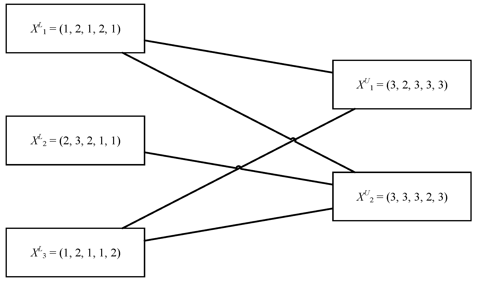
Input: all $X_i^L$ and $X_j^U$: $X_1^L$ = (1, 2, 1, 2, 1), $X_2^L$ = (2, 3, 2, 1, 1), $X_3^L$ = (1, 2, 1, 1, 2), and $X_1^U$ = (3, 2, 3, 3, 3) and $X_2^U$ = (3, 3, 3, 2, 3).

Set η = True and RG = 0.

Since the condition |$X_j^U$| ≤ |$X_i^L$| is true, apply Equation (11) to calculate RG.

Set R1 = 0.

FORS1

Set ${\overline{M}}^1$ = $X_1^U$ = (3, 2, 3, 3, 3).

From the relationship, $I_1^1=1$, $I_2^1=0$, $I_3^1=1$.

Pr(S1) = Pr(${\displaystyle {\cup }_{i:1,3}^{}\left\{X\right|X_i^L\le X\le {\overline{M}}^1\}}$) = 0.8457.

R1 ← R1 + Pr(S1) = 0.8457

FORS2

Set ${\overline{M}}^2$ = $X_2^U$ = (3, 3, 3, 2, 3).

From the relationship, $I_1^2=1$, $I_2^2=1$, $I_3^2=1$.

Pr(S2) = Pr(${\displaystyle {\cup }_{i:1,2,3}^{}\left\{X\right|X_i^L\le X\le {\overline{M}}^2\}}$) = 0.7555.

R1 ← R1 + Pr(S2) = 1.6013

END FOR

RG ← RG + R1 = 1.6013

η = False //reverse the flag.

FOR p = 2 //the second term $\mathrm{Pr}(S_{{\theta }_1}\cap S_{{\theta }_2})$

Set R2 = 0.

FOR S1, S2 //the first combination with two Sj

Set ${\overline{M}}^2$ = $X_1^U$ ↓ $X_2^U$= (3, 2, 3, 2, 3).

From the relationships, $I_1^1=1$, $I_2^1=0$, $I_3^1=1$ and $I_1^2=1$, $I_2^2=1$, $I_3^2=1$.  Pr(S1 ∩ S2) = Pr(${\displaystyle {\cup }_{i:1,3}^{}\left\{X\right|X_i^L\le X\le {\overline{M}}^2\}}$) = 0.6757.

R2 ← R2 + Pr(S1 ∩ S2) = 0.6757

END FOR

RG ← RG − R2 = 0.9255

I = True //reverse the flag.

Output: RG = 0.9255

In the numerical example, SFN reliability R_G is 0.9255. By the enumeration approach, 3⁵ = 243 capacity vectors are listed from (1, 1, 1, 1, 1) to (3, 3, 3, 3, 3) firstly. Each vector is confirmed whether to be feasible. Finally, the probabilities of every feasible state vector are added up to obtain R_G. On the contrary, the proposed algorithm only calculates Pr(S₁), Pr(S₂), and Pr(S₁ ∩ S₂), to obtain R_G, with the corresponding shared upper boundary point.

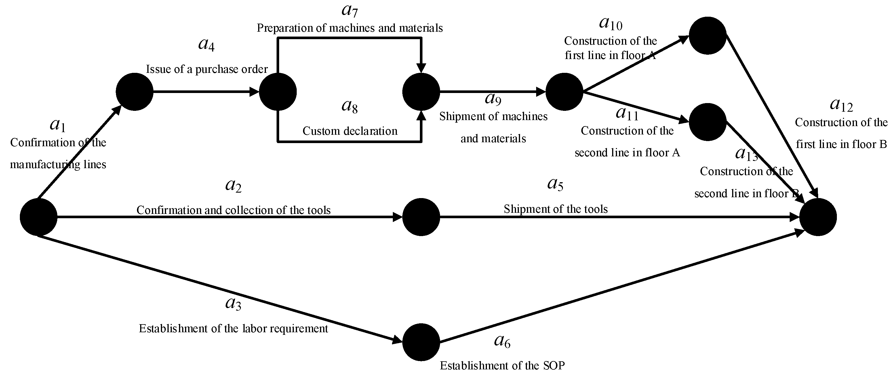
6. Case Study

This section studies a notebook manufacturer whose headquarters is located in Taiwan. The manufacturer is planning to launch a construction project of new manufacturing lines in Chengdu, China. A project manager plans to ensure that the project can be completed within the expected time and budget. By executing the algorithm in literature [10], the upper and lower boundary points can be generated in terms of different times and budgets, respectively.

In detail, the project consists of 13 main activities, and the project is transformed to an SFN as shown in Figure 2. The durations and the corresponding cost of each activity are displayed in

Table 2. Durations, costs, and probabilities of each activity.

Arc	Activity	Duration (Days)	Cost (CNY)	Probability
a1	Confirmation of the manufacturing lines	3	4500	0.20
		5	3000	0.40
		7	1500	0.40
a2	Confirmation and collection of the tools	2	8400	0.10
		7	4200	0.70
		10	3000	0.20
a3	Establishment of the labor requirement	7	4500	0.10
		14	3000	0.60
		21	1500	0.30
a4	Issue of a purchase order	14	2400	0.10
		28	1200	0.70
		42	600	0.20
a5	Shipment of the tools	20	20,000	0.70
		30	15,000	0.30
a6	Establishment of the SOP	7	1800	0.20
		14	1200	0.70
		18	600	0.10
a7	Preparation of machines and materials	12	7200	0.05
		14	6000	0.90
		16	4800	0.05
a8	Custom declaration	14	1200	0.20
		21	600	0.80
a9	Shipment of machines and materials	21	40,000	0.70
		31	30,000	0.30
a10	Construction of the first line in floor A	11	10,200	0.05
		18	9000	0.05
		25	7400	0.90
a11	Construction of the second line in floor A	5	10,200	0.05
		12	9000	0.05
		19	7400	0.90
a12	Construction of the first line in floor B	7	10,200	0.05
		14	9000	0.05
		21	7400	0.90
a13	Construction of the second line in floor B	5	10,200	0.05
		12	9000	0.05
		19	7400	0.90

.

Table 3. Experimental results.

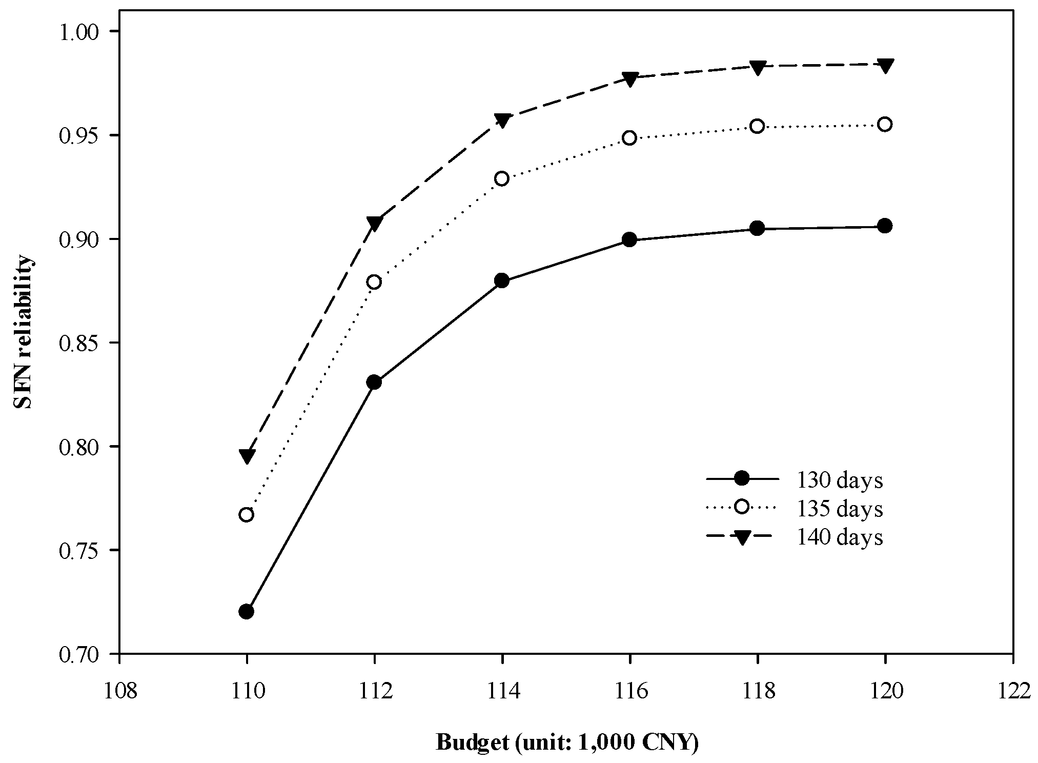
	Time (Unit: Day)
Budget Unit: 1000 CNY	130	135	140
110	0.565067	0.721672	0.772429
112	0.669611	0.832017	0.884594
114	0.71561	0.881236	0.934397
116	0.734547	0.900869	0.954106
118	0.739934	0.906411	0.959655
120	0.740957	0.907454	0.960698

shows the experimental results from 130 to 140 days and from 110,000 to 120,000 (CNY). Besides, Figure 3 presents the patterns of project reliability in terms of the time and budget. Suppose, under 112,000 CNY and 140 days, the project can be completed with 88.4594% probability. The experimental results also provide the managers with managerial implications. For instance, suppose that the managers plan to guarantee SFN reliability 0.9 under 135 days. The minimum budget should be 116,000.

7. Conclusions

SFN reliability R_G is utilized for quality evaluation of the stochastic flow networks (SFN) and is defined as the probability of all feasible capacity vectors, satisfying certain constraints, such as demand, cost or time, etc. However, for the probability calculation, previous researches, including the improved recursive sum of disjoint products [14] and state space decomposition [15,16], focused on the unilateral boundary points. In some certain cases, upper and lower boundary points, $X_j^U$ and $X_i^L$, are necessary to apply at the same time. For instance, there are time and budget constraints in the literature [10] considered to generate $X_j^U$ and $X_i^L$, simultaneously. It is a challenge to calculate the probabilities of the capacity vectors contained in $X_j^U$ and $X_i^L$ to obtain R_G due to the complex relationships.

In order to evaluate SFN reliability with $X_j^U$ and $X_i^L$, this paper proposes a decomposition of the feasible areas into several subsets S_j to calculate R_G in terms of an $X_j^U$. For computational efficiency, the relationships between $X_j^U$ and all $X_i^L$ in S_j is formulated to reduce the computational loading. Then, SFN reliability R_G is formatted as the inclusion-exclusion principle by means of S_j. To calculate the probability of each term in the inclusion-exclusion principle with S_j, a special “minimum” operator termed “ ↓” is developed to generate a shared boundary vector such that each term only has one unilateral boundary point. Finally, two heuristic options for the shared boundary points are established to calculate R_G in an efficient direction. The main merit of the heuristic options is to generate less terms for the calculation of R_G such that the computational loading is mitigated.

It is suggested that by using the proposed algorithm with the lower and upper boundary points, the reliability evaluation can be addressed for practical issues: the required flow between two different demands and project reliability with time and budget constraints.

References

- Yeh, W.C.; Chu, T.C. A novel multi-distribution multi-state flow network and its reliability optimization problem. Reliab. Eng. Syst. Saf. 2018, 176, 209–217. [Google Scholar] [CrossRef]
- Huang, C.F. Evaluation of system reliability for a stochastic delivery-flow distribution network with inventory. Ann. Oper. Res. 2019, 277, 33–45. [Google Scholar] [CrossRef]
- Lin, Y.K.; Huang, D.H. Reliability analysis for a hybrid flow shop with due date consideration. Reliab. Eng. Syst. Saf. 2017. [Google Scholar] [CrossRef]
- Chang, P.C. Reliability estimation for a stochastic production system with finite buffer storage by a simulation approach. Ann. Oper. Res. 2017, 277, 119–133. [Google Scholar] [CrossRef]
- Schneider, K.; Rainwater, C.; Pohl, E.; Hernandez, I.; Ramirez-Marquez, J.E. Social network analysis via multi-state reliability and conditional influence models. Reliab. Eng. Syst. Saf. 2013, 109, 99–109. [Google Scholar] [CrossRef]
- Lin, Y.K.; Huang, C.F. A multi-state computer network within transmission error rate and time constraints. J. Chin. Inst. Ind. Eng. 2012, 29, 477–484. [Google Scholar] [CrossRef]
- Yeh, C.T.; Fiondella, L. Optimal redundancy allocation to maximize multi-state computer network reliability subject to correlated failures. Reliab. Eng. Syst. Saf. 2017, 166, 138–150. [Google Scholar] [CrossRef]
- Lin, Y.K.; Pan, C.L. Considering retransmission mechanism and latency for network reliability evaluation in a stochastic computer network. J. Ind. Prod. Eng. 2014, 31, 350–358. [Google Scholar] [CrossRef]
- Yeh, C.T. An improved NSGA2 to solve a bi-objective optimization problem of multi-state electronic transaction network. Reliab. Eng. Syst. Saf. 2019, 191, 106578. [Google Scholar] [CrossRef]
- Lin, Y.K. Project management for arbitrary random durations and cost attributes by applying network approaches. Comput. Math. Appl. 2008, 56, 2650–2655. [Google Scholar] [CrossRef]
- Zarezadeh, S.; Ashrafi, S.; Asadi, M. Network Reliability Modeling Based on a Geometric Counting Process. Mathematics 2018, 6, 197. [Google Scholar] [CrossRef]
- El Khadiri, M.; Yeh, W.C. An efficient alternative to the exact evaluation of the quickest path flow network reliability problem. Comput. Oper. Res. 2016, 76, 22–32. [Google Scholar] [CrossRef]
- Niu, Y.F.; Xu X, Z. Reliability evaluation of multi-state systems under cost consideration. Appl. Math. Model. 2012, 36, 4261–4270. [Google Scholar] [CrossRef]
- Bai, G.H.; Zuo, M.J.; Tian, Z.G. Ordering heuristics for reliability evaluation of multistate networks. IEEE Trans. Reliab. 2015, 64, 1015–1023. [Google Scholar] [CrossRef]
- Aven, T. Reliability evaluation of multistate systems with multistate components. IEEE Trans. Reliab. 1985, 34, 473–479. [Google Scholar] [CrossRef]
- Bai, G.; Tian, Z.; Zuo, M.J. Reliability evaluation of multistate networks: An improved algorithm using state-space decomposition and experimental comparison. IISE Trans. 2018, 50, 407–418. [Google Scholar] [CrossRef]
- Yeh, W.C. An improved sum-of-disjoint-products technique for the symbolic network reliability analysis with known minimal paths. Reliab. Eng. Syst. Saf. 2007, 92, 260–268. [Google Scholar] [CrossRef]