Removing Twins in Graphs to Break Symmetries

Abstract

Determining vertex subsets are known tools to provide information about automorphism groups of graphs and, consequently about symmetries of graphs. In this paper, we provide both lower and upper bounds of the minimum size of such vertex subsets, called the determining number of the graph. These bounds, which are performed for arbitrary graphs, allow us to compute the determining number in two different graph families such are cographs and unit interval graphs.

1. Introduction and Preliminaries

The graph isomorphism problem is not known to be solvable in polynomial time nor to be NP-complete (see [1]) and moreover, it is well known that constructing the automorphism group is at least as difficult (in terms of computational complexity) as solving the graph isomorphism problem (see [2]). Therefore, it is interesting to provide tools that give information about such automorphism groups.

Determining sets were introduced simultaneously by Boutin [3] and Erwin and Harary [4] (they called them fixing sets) in 2006, to deal with the problem of identifying the automorphism group of a graph. These sets are a generalization of resolving sets, independently introduced by Slater [5] and Harary and Melter [6], motivated by the problem of identifying the location of an intruder in a network, by means of distances. Resolving sets and some related sets were recently studied in [7,8,9,10,11,12]. Determining sets and resolving sets were jointly studied (see [13,14]). Furthermore, determining sets are closely related to the notion of “symmetry breaking”, firstly studied by Alberson and Collins [15] in 1996. The interest of this notion, beyond the information it provides about the automorphism group, was pointed out by Bailey and Cameron in their survey paper [16] of 2011, citing Babai’s words [17]:

“In fact, breaking regularity is one of the key tools in the design of algorithms for graph isomorphism; the graph isomorphism problem has therefore been one of the strongest motivators of the study of all sorts of resolving/discriminating sets, and perhaps the only deep motivator of the study of those in contexts where no group is present.”

In this paper, we deepen the study of determining sets of general graphs, providing both lower and upper bounds of this parameter in terms of the so-called twin graph. We follow the same spirit as other works that find general bounds involving other aspects of graphs, such as the number of automorphisms [3] or the number of orbits [4]. Furthermore, our bounds allow us to obtain the determining number of some graph classes (cographs and unit interval graphs), which is a problem of interest due to the NP-hardness of the computation of this parameter in arbitrary graphs [18]. Indeed, many papers in the literature are devoted to study the determining number of specific graph families: trees [4,13], Cartesian products [4,13,19], Kneser and Johnson graphs [3,20], twin-free graphs [14], and Cayley graphs [21]; among others.

We now introduce the definitions and notations that we shall need throughout the rest of the paper. All graphs considered here are finite, simple and undirected. An automorphism of a graph G is a bijective mapping $\varphi :V(G)⟶V(G)$ so that $\varphi (u)\varphi (v)\in E(G)$ if and only if $uv\in E(G)$. The set $\mathrm{Aut}(G)$ of all automorphisms of G forms a group under composition, and its identity element is denoted by $i{d}_G$. We recall the definition of determining set and determining number from [3].

Definition 1

([3]). A subset S of the vertices of a graph G is called a determining set if whenever $g,h\in \mathrm{Aut}(G)$ agree on the vertices of S, they agree on all vertices of G. That is, S is a determining set if whenever g and h are automorphisms with the property that $g(s)=h(s)$ for all $s\in S$, then $g=h$. The determining number of a graph G is the smallest integer r so that G has a determining set of size r. Denote this by $\mathrm{Det}(G)$.

We quote from [3] the following example illustrating this concept.

Example 1.

The Petersen graph is shown in Figure 1, where the vertices are identified with the 2-subsets of a 5-set. The Persersen graph has a determining number equal to three and examples of minimum determining sets of this graph are $S=\{\{1,2\},\{2,4\},\{2,5\}\}$ and $T=\{\{1,2\},\{2,3\},\{3,4\}\}$ (see [3]).

The following useful characterization of determining sets, in terms of the stabilizer of a vertex subset, can be also found in [3]. The stabilizer of a vertex subset $S\subseteq V(G)$ is the automorphism subset ${\mathrm{Stab}}_G(S)=\{\varphi \in \mathrm{Aut}(G):\varphi (u)=u,\forall u\in S\}$. Observe that ${\mathrm{Stab}}_G(S)={\bigcap }_{s\in S}{\mathrm{Stab}}_G(\{s\})$, and moreover $S\subseteq T$ implies that ${\mathrm{Stab}}_G(T)\subseteq {\mathrm{Stab}}_G(S)$.

Proposition 1

([3]). Let S be a subset of the vertices of a graph G. Then S is a determining set of G if and only if ${\mathrm{Stab}}_G(S)=\{i{d}_G\}$.

We now quote from [22] the construction of the twin graph $G^1$ associated with a given graph G. This graph will be the main tool to obtain our new bounds. For a vertex $u\in V(G)$, the open and the closed neighborhood of u are respectively denoted by $N(u)$ and $N\left[u\right]$ and the degree of u is $deg(u)=|N(u)|$. We say that two different vertices $u,v\in V(G)$ are twins when $N(u)=N(v)$ or $N\left[u\right]=N\left[v\right]$. This notion induces the following equivalence relation on $V(G)$: $u\equiv v$ if and only if either $u=v$ or u and v are twins. This allows defining the twin class of u as $\left[u\right]=\{v\in V(G):u\equiv v\}$. We say that a twin class is trivial if it contains just one vertex and non-trivial in other case. When each twin class is trivial, we say that G is twin-free. For $S\subseteq V(G)$, we write $\left[S\right]={\cup }_{u\in S}\left[u\right]$.

Assuming that there are exactly $n^{(1)}$ different equivalence classes, we can consider the partition $\left[u_1\right],\dots ,\left[u_{n^{(1)}}\right]$ of $V(G)$ induced by them, where every $u_i$ is a representative of $\left[u_i\right]$. The twin graph of G, denoted by $G^1$, is the graph with vertex set the set of equivalence classes of G. The vertex of $G^1$ representing the equivalence class $\left[u\right]$ is denoted by $u^1$. The edge set is $E(G^1)=\{u^1{v}^1:uv\in E(G)\}$. For $S\subseteq V(G)$, we denote $S^1=\{u^1\in V(G^1):u\in S\}$.

Please note that $G^1$ is well defined, as shown in the following lemma.

Lemma 1

([22]). Let $G^1$ be the twin graph of a graph G. Then, $u^1{v}^1\in E(G^1)$ if and only if $xy\in E(G)$ for all $x\in \left[u\right]$, $y\in \left[v\right]$.

We illustrate the construction of the twin graph of a given graph G with the following example.

Example 2.

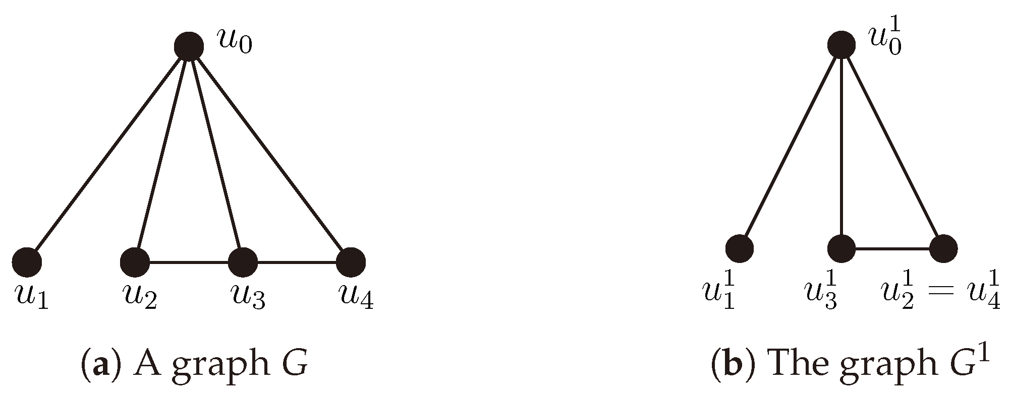
A graph G and its twin graph$G^1$are shown in Figure 2a,b, respectively. Please note that$u_2$and$u_4$are twin vertices of G, so$u_2^1=u_4^1$in$G^1$.

This paper is organized as follows. In Section 2 we use the twin graph $G^1$ to provide a lower bound of the determining number of an arbitrary graph G, whereas in Section 3 we use similar tools to give an upper bound. Section 4 is devoted to use these bounds to compute the determining number of cographs and unit interval graphs. We conclude the paper in Section 5 with some remarks and future work.

2. A Lower Bound of $\mathbf{Det}(\mathit{G})$ from Removing Twins

In this section, we present a new lower bound of the determining number of a graph. A lower bound in terms of both orders of G and $G^1$ is already known (see [14]).

Lemma 2

([14]). Let G be a graph of order n such that $G^1$ has order $n^{(1)}$. Then,

$$n-n^{(1)}\le \mathrm{Det}(G).$$

We present a different approach that relates the determining numbers of G and $G^1$. To this end, we need to define the following natural mapping between the automorphism groups of both G and $G^1$:

$$\tilde{\mathcal{T}}:\mathrm{Aut}(G)\to \mathrm{Aut}(G^1)$$

given by $\tilde{\mathcal{T}}(\varphi )(u^1)=\varphi {(u)}^1$. In the following lemma, we show that this mapping is a well-defined group automorphism.

Lemma 3.

For every graph G, the mapping$\tilde{\mathcal{T}}$satisfies the following properties:

1. 

$\tilde{\mathcal{T}}$is well-defined.

2. 

$\tilde{\mathcal{T}}$is a group homomorphism.

Proof. 

• Firstly, we have to check that $\tilde{\mathcal{T}}(\varphi )(u^1)$ does not depend on the choice of the representative of $u^1$. By definition of graph automorphism, it is clear that $N(u)=N(v)$ if and only if $N(\varphi (u))=N(\varphi (v))$, and also $N\left[u\right]=N\left[v\right]$ if and only if $N[\varphi (u)]=N[\varphi (v)]$, so $u,v$ are twin vertices if and only of $\varphi (u),\varphi (v)$ are twin vertices. Let $u,v\in V(G)$ be two different vertices such that $v^1=u^1$, then $u,v$ are twin vertices and $\varphi (v),\varphi (u)$ are also twin vertices, that means that $\varphi {(v)}^1=\varphi {(u)}^1$. Therefore ${\tilde{\mathcal{T}}}_G(\varphi )(u^1)=\varphi {(u)}^1=\varphi {(v)}^1=\tilde{\mathcal{T}}(\varphi )(v^1)$.
  On the other hand, for $u^1,v^1\in V(G^1)$, Lemma 1 yields $u^1{v}^1\in E(G^1)$ if and only if $uv\in E(G)$, or equivalently $\varphi (u)\varphi (v)\in E(G)$, that is $\varphi {(u)}^1\varphi {(v)}^1=\tilde{\mathcal{T}}(\varphi )(u^1)\tilde{\mathcal{T}}(\varphi )(v^1)\in E(G^1)$, as desired.
• Clearly $\tilde{\mathcal{T}}(\varphi \circ {\varphi }^{\prime })(u^1)=(\varphi \circ {\varphi }^{\prime }){(u)}^1=\varphi {({\varphi }^{\prime }(u))}^1=\tilde{\mathcal{T}}(\varphi )({\varphi }^{\prime }{(u)}^1)=\tilde{\mathcal{T}}(\varphi )\circ \tilde{\mathcal{T}}({\varphi }^{\prime })(u^1)$, so $\tilde{\mathcal{T}}(\varphi \circ {\varphi }^{\prime })=\tilde{\mathcal{T}}(\varphi )\circ \tilde{\mathcal{T}}({\varphi }^{\prime })$. □

We will also need the following definition of a special type of vertex subset. We say that a set $\Omega \subseteq V(G)$ is a plenty twin set if no pair of vertices of $V(G)\setminus \Omega$ are twins. Equivalently, $\Omega$ is a plenty twin set if it contains all but at most one vertices of every non-trivial twin class. In particular, this gives that every determining set is a plenty twin set (see [14], proof of Lemma 3.3). However, there are plenty twin sets that are not determining sets, as we show with the following example.

Example 3.

The graph G in Figure 3 has exactly two non-trivial twin classes,$\left[u_1\right]=\{u_1,v_1\},\left[u_2\right]=\{u_2,v_2\}$, therefore$\{u_1,u_2\}$is a plenty twin set. Moreover, the mapping φ satisfying$\varphi (w)=w$for every vertex$w\in \{u,u_1,v_1,u_2,v_2\}$,$\varphi (a_1)=a_2,\varphi (a_2)=a_1,\varphi (b_1)=b_2,\varphi (b_2)=b_1$is a non-trivial graph automorphism fixing both$u_1,u_2$, so$\{u_1,u_2\}$is not a determining set of G.

A basic property of plenty twin sets is the following.

Lemma 4.

If Ω is a plenty twin set of a graph G, then${\Omega }^1$is a plenty twin set of$G^1$.

Proof. 

On the contrary, let us assume that there is a pair of twins $x^1,y^1\in V(G^1)\setminus {\Omega }^1$. Thus, we have that $x,y\in V(G)\setminus [\Omega ]$, and so $\left[x\right]=\{x\}$ and $\left[y\right]=\{y\}$, because $\Omega$ is a plenty twin set.

In particular, $x,y$ are not twins in G, and so we may assume without loss of generality the existence of a vertex $z\in V(G)\setminus \{x,y\}$ such that $z\in N_G(x)$ and $z\notin N_G(y)$. By Lemma 1, $z^1\in N_{G^1}(x^1)$ and $z^1\notin N_{G^1}(y^1)$. This contradicts the fact that $x^1$ and $y^1$ are twins. □

In the following lemma, we present the general behaviour of the stabilizer of a vertex subset under the mapping $\tilde{\mathcal{T}}$ and also the special situation of plenty twin sets.

Lemma 5.

Let G be a graph. For any subset$S\subseteq V(G)$, it holds that

$$\tilde{\mathcal{T}}({\mathrm{Stab}}_G(S))\subseteq {\mathrm{Stab}}_{G^1}(S^1).$$

Furthermore, if S is a plenty twin set, then the equality holds.

Proof. 

Let $\varphi \in \mathrm{Aut}(G)$ such that $\varphi (u)=u$ for all $u\in S$. Thus, $\tilde{\mathcal{T}}(\varphi )(u^1)=\varphi {(u)}^1=u^1$, and so $\tilde{\mathcal{T}}(\varphi )\in {\mathrm{Stab}}_{G^1}(S^1)$, which gives the desired inclusion.

Now, assume that S is a plenty twin set and let $\psi \in {\mathrm{Stab}}_{G^1}(S^1)$, and let us construct the mapping $\varphi :V(G)⟶V(G)$ in the following way. If $u\in V(G)$ satisfies $u^1\in S^1$ then we define $\varphi (u)=u$ (in particular $\varphi (u)=u$ for all $u\in S$). In this case, it is clear that $\psi (u^1)=u^1=\varphi {(u)}^1$. On the other hand, if $u\in V(G)$ satisfies $u^1\in V(G^1)\setminus S^1$ then, $\psi (u^1)\in V(G^1)\setminus S^1$, because $\psi \in {\mathrm{Stab}}_{G^1}(S^1)$. Thus there exists $v^1\in V(G^1)\setminus S^1$ such that $\psi (u^1)=v^1$. Using that S is a plenty twin set, we obtain that $\left[v\right]=\{v\}$, and we define $\varphi (u)=v$. Please note that in this case, again $\psi (u^1)=v^1=\varphi {(u)}^1$.

Let us check that $\varphi$ is an automorphism of G. Indeed, $uv\in E(G)$ if and only if $u^1{v}^1\in E(G^1)$, which is equivalent to $\varphi {(u)}^1\varphi {(v)}^1=\psi (u^1)\psi (v^1)\in E(G^1)$ since $\psi$ is an automorphism of $G^1$. Again, this is equivalent to $\varphi (u)\varphi (v)\in E(G)$, by Lemma 1. This proves that $\varphi \in \mathrm{Aut}(G)$.

By construction, $\psi (u^1)=\varphi {(u)}^1=\tilde{\mathcal{T}}(\varphi )(u^1)$ for all $u\in V(G)$, and so $\psi =\tilde{\mathcal{T}}(\varphi )$. Furthermore, $\varphi$ fixes each element of S, which means $\varphi \in {\mathrm{Stab}}_{\mathrm{G}}(\mathrm{S})$. Therefore, $\tilde{\mathcal{T}}({\mathrm{Stab}}_G(S))\supseteq {\mathrm{Stab}}_{G^1}(S^1)$. □

We now present the announced lower bound of the determining number of a graph, in terms of the corresponding parameter of its twin graph.

Theorem 1.

If S is a determining set of a graph G then$S^1$is a determining set of the twin graph$G^1$. Consequently,$\mathrm{Det}(G^1)\le \mathrm{Det}(G)$and this bound is tight.

Proof. 

Let S be a determining set of G. Thus, S is a plenty twin set and Lemma 5 gives

$${\tilde{\mathcal{T}}}_G({\mathrm{Stab}}_G(S))={\mathrm{Stab}}_{G^1}(S^1).$$

(1)

On the other hand, $\tilde{\mathcal{T}}$ is a group homomorphism and ${\mathrm{Stab}}_G(S)=\{i{d}_G\}$, which implies that $\tilde{\mathcal{T}}({\mathrm{Stab}}_G(S))=\tilde{\mathcal{T}}(\{i{d}_G\})=\{i{d}_{G^1}\}.$ Combining this with Equality (1), we obtain that ${\mathrm{Stab}}_{G^1}(S^1)=\{i{d}_{G^1}\}$ and $S^1$ is a determining set of $G^1$. Furthermore, $|S^1|\le |S|$ and therefore $\mathrm{Det}(G^1)\le \mathrm{Det}(G)$.

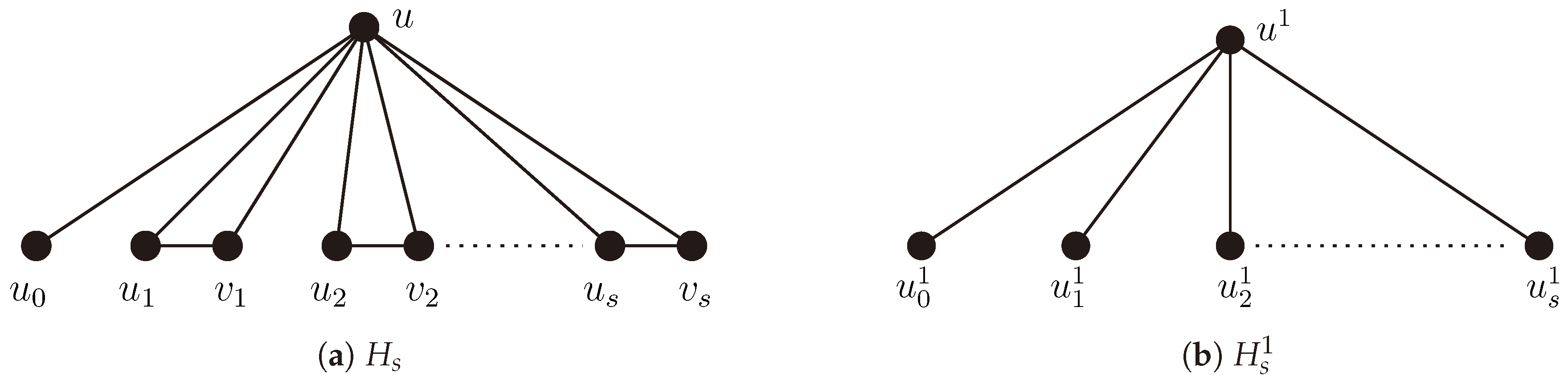
To prove the tightness of the bound, let $H_s$, with $s\ge 1$, be a graph with vertex set $V(H_s)=\{u,u_0\}\cup \{u_1,v_1,\dots ,u_s,v_s\}$ and edge set $E(H_s)=\{u{u}_i:0\le i\le s\}\cup \{u{v}_i:1\le i\le s\}\cup \{u_i{v}_i:1\le i\le s\}$; its twin graph $H_s^1$ is a star on $s+2$ vertices (see Figure 4). It is easy to check that $S=\{u_1,\dots ,u_s\}$ and $S^1=\{u_1^1,\dots ,u_s^1\}$ are minimum determining sets of $H_s$ and $H_s^1$, respectively, and so $\mathrm{Det}(H_s)=\mathrm{Det}(H_s^1)=s$. □

In order to compare our new lower bound with that showed in Lemma 2, we provide the following two examples.

Example 4.

Consider the graph G with$s+2$ vertices consisting of a complete graph with $s\ge 3$ vertices, a vertex v that is not a neighbor of any vertex in the complete graph and a vertex u which is a neighbor of v and of every vertex in the complete graph (see Figure 5a). Clearly $G^1$ is a path with three vertices (see Figure 5b), so $n^{(1)}=3$ and $\mathrm{Det}(G^1)=1$. Therefore $\mathrm{Det}(G^1)=1<n-n^{(1)}=s+2-3=s-1$ and in this case, the lower bound in Lemma 2 is greater than the new one.

Example 5.

Consider the graph G, with$n=3s+3$vertices ($s\ge 3$), shown in Figure 6a, whose twin graph$G^1$is depicted in Figure 6b. In this case,$n^{(1)}=n-1$and$S=\{u_1^1,u_2^1,\cdots u_{s-1}^1\}$is a minimum determining set of$G^1$, so$\mathrm{Det}(G^1)=s-1$. Therefore$n-n^{(1)}=1<\mathrm{Det}(G^1)$and our new lower bound is a better option than the old one.

Therefore, both lower bounds are independent and we obtain the following corollary.

Corollary 1.

Let G be a graph. Then, it holds that

$$max\{n-n^{(1)},\mathrm{Det}(G^1)\}\le \mathrm{Det}(G).$$

3. An Upper Bound on $\mathbf{Det}(\mathit{G})$ from Removing Twins

In the previous section, we explored the relationship between the determining number of graphs G and $G^1$, and thereby providing a new general lower bound for the determining number of a graph. We now focus on using such relationship to obtain an upper bound for the determining number.

Our strategy is now to obtain a twin-free graph by iterating the process of building $G^1$ from G. Contrary to what one might think, the twin graph $G^1$ of a graph G is not twin-free in general (see Figure 7).

This fact suggests the iterative process of defining, for any integer $i\ge 2$, the graph $G^i$ as the twin graph of $G^{i-1}$; its order is denoted by $n^{(i)}$. So, having in mind that G is a finite graph, we can iterate this process thus obtaining a graph sequence $G=G^0,G^1,\dots ,G^r$, where $G^r$ is the only twin-free graph of the sequence. Clearly, if G is a non twin-free graph with n vertices, then $1\le r\le n-1$. The following example illustrates the extreme case $r=n-1$.

Example 6.

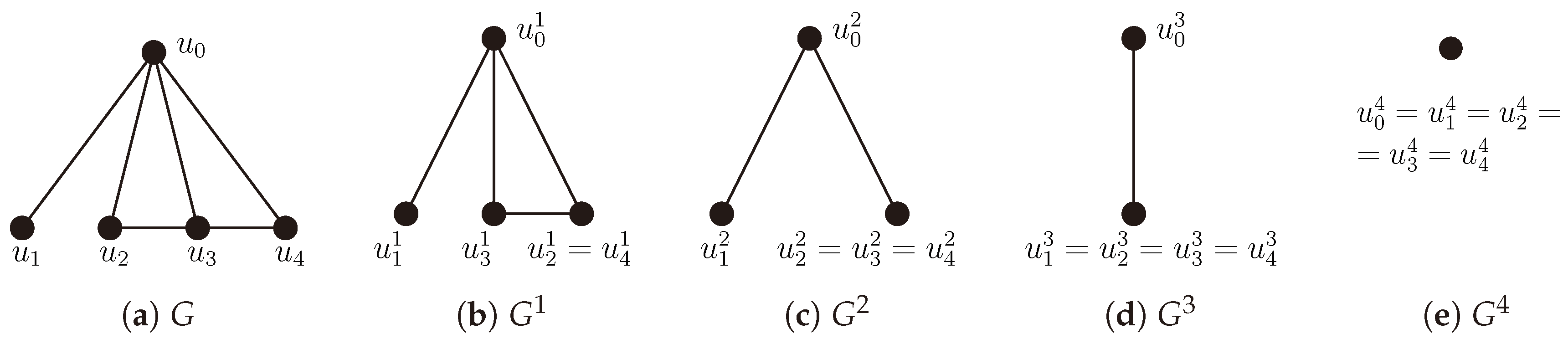
In Figure 8 we show a graph G with$n=5$vertices, and its sequence of twin graphs$G^1,G^2,G^3,G^4$. Please note that$G,G^1,G^2,G^3$are not twin-free whereas$G^4$is, so$r=4=5-1=n-1$.

We denote by ${\mathcal{T}}^i:V(G^{i-1})\to V(G^i)$ the natural projection of $G^{i-1}$ onto its twin graph $G^i$, for any $1\le i\le r$. Let us denote $u^i=({\mathcal{T}}^i\circ {\mathcal{T}}^{i-1}\circ \dots \circ {\mathcal{T}}^1)(u)$ and ${\left[u\right]}^i=\{v\in V(G):u^i=v^i\}$ for any vertex $u\in V(G)$. In general, for any subset $S\subseteq V(G)$, we denote by $S^i=\{u^i\in V(G^i):u\in S\}$, note that it is a vertex subset of $G^i$, and by ${\left[S\right]}^i=\{u\in V(G):u^i\in S^i\}$, note that it is a vertex subset of G.

The proof of the following properties is trivial.

Lemma 6.

Let G be a graph, let$u\in V(G)$and let$S\subseteq V(G)$. Then, the following statements hold

1. 

${\left[u\right]}^1=\left[u\right]$and${\left[S\right]}^1=\left[S\right]$.

2. 

$\left[u\right]\subseteq {\left[u\right]}^i$and this inclusion is not an equality in general, for$i\ge 2$.

3. 

$S\subseteq {\left[S\right]}^1\subseteq {\left[S\right]}^2\subseteq \dots \subseteq {\left[S\right]}^r\subseteq V(G)$. In particular, if S is a plenty twin set, then${\left[S\right]}^i$is also a plenty twin set, for every i.

Remark 1.

In Figure 8 we can see an example of the second property of Lemma 6. In this case${\left[u_4\right]}^1=\{u_2,u_4\}⊊{\left[u_4\right]}^2=\{u_2,u_3,u_4\}⊊{\left[u_4\right]}^3=\{u_1,u_2,u_3,u_4\}⊊{\left[u_4\right]}^4=\{u_0,u_1,u_2,u_3,u_4\}$.

The iterated application of the construction process of the twin graph easily provides this straightforward generalization of Lemma 4.

Lemma 7.

If Ω is a plenty twin set of a graph G, then${\Omega }^i$is a plenty twin set of$G^i$, for$i\ge 1$.

We now present three technical lemmas that will be useful to obtain the main result of this section. These lemmas collect the behavior of plenty twin sets and their stabilizers under the successive twin graph operations.

Lemma 8.

Let Ω be a plenty twin set of a graph G, and let$x\in V(G)$. If$x\in V(G)\setminus {[\Omega ]}^i$for some$i\ge 1$, then${\left[x\right]}^i=\{x\}$.

Proof. 

We proceed by induction on $i\ge 1$. For $i=1$, let $x\in V(G)\setminus {[\Omega ]}^1=V(G)\setminus [\Omega ]$; in particular, $x\notin \Omega$. Suppose on the contrary that there exists $y\ne x$ such that $y\in {\left[x\right]}^1=\left[x\right]$. Then, x and y are twin vertices of G, and using that $\Omega$ is a plenty twin set, we obtain that $y\in \Omega$. However, this means $x\in \left[y\right]\subseteq [\Omega ]$, which is a contradiction.

Our inductive hypothesis is the following: if $x\in V(G)\setminus {[\Omega ]}^{i-1}$ then ${\left[x\right]}^{i-1}=\{x\}$. Suppose now that $x\in V(G)\setminus {[\Omega ]}^i$ (and so $x^i\notin {\Omega }^i$ by definition of ${\Omega }^i$); in particular, by Statement 3 of Lemma 6, $x\notin {[\Omega ]}^{i-1}$ (and so $x^{i-1}\notin {\Omega }^{i-1}$) and by the inductive hypothesis ${\left[x\right]}^{i-1}=\{x\}$. Assume that there exists $y\ne x$ such that $y\in {\left[x\right]}^i$, which yields $x^i=y^i$. This implies that $x^{i-1}$ and $y^{i-1}$ are twins in $G^{i-1}$. We know that ${\left[x\right]}^{i-1}=\{x\}$, so $y^{i-1}\ne x^{i-1}$. On the other hand, ${\Omega }^{i-1}$ is a plenty twin set because of Lemma 7, so $y^{i-1}\in {\Omega }^{i-1}$. Finally, this gives that $x^i=y^i\in {\Omega }^i$, a contradiction. □

Lemma 9.

Let Ω be a plenty twin set of a graph G. Then, for every$i\ge 1$,

$${\mathrm{Stab}}_{G^{i-1}}({\Omega }^{i-1})={\mathrm{Stab}}_{G^{i-1}}({({\mathcal{T}}^i)}^{-1}({\Omega }^i)).$$

Proof. 

Recall that $G^0=G$ and ${\Omega }^0=\Omega$. We only have to prove the inclusion ${\mathrm{Stab}}_{G^{i-1}}({\Omega }^{i-1})\subseteq {\mathrm{Stab}}_{G^{i-1}}({({\mathcal{T}}^i)}^{-1}({\Omega }^i))$, so let $\varphi \in {\mathrm{Stab}}_{G^{i-1}}({\Omega }^{i-1})$ and let $u^{i-1}\in {({\mathcal{T}}^i)}^{-1}({\Omega }^i)$. We need to show that $\varphi (u^{i-1})=u^{i-1}$. If $u_{i-1}\in {\Omega }^{i-1}$, then $\varphi (u^{i-1})=u^{i-1}$, by hypothesis about $\varphi$. Assume now that $u_{i-1}\in {({\mathcal{T}}^i)}^{-1}({\Omega }^i)\setminus {\Omega }^{i-1}$. Then ${\mathcal{T}}^i(u^{i-1})=u^i\in {\Omega }^i$.

On the other hand, $\varphi \in {\mathrm{Stab}}_{G^{i-1}}({\Omega }^{i-1})$ implies that ${\tilde{\mathcal{T}}}^i(\varphi )\in {\tilde{\mathcal{T}}}^i({\mathrm{Stab}}_{G^{i-1}}({\Omega }^{i-1}))={\mathrm{Stab}}_{G^i}({\Omega }^i)$, by Lemma 5, and so ${\tilde{\mathcal{T}}}^i(\varphi )(u^i)=u^i$. Moreover, by definition, ${\tilde{\mathcal{T}}}^i(\varphi )(u^i)={(\varphi (u^{i-1}))}^1$, and this means that ${(\varphi (u^{i-1}))}^1=u^i$. In other words, $\varphi (u^{i-1})$ and $u^{i-1}$ belong to the same twin class in $G^{i-1}$.

Finally, if $\varphi (u^{i-1})\ne u^{i-1}$, using that ${\Omega }^{i-1}$ is a plenty twin set not containing $u^{i-1}$, we have that $\varphi (u^{i-1})\in {\Omega }^{i-1}$, however this is not possible because $\varphi$ is a bijective mapping that fixes every vertex in ${\Omega }^{i-1}$, and no vertex outside ${\Omega }^{i-1}$ have its image in ${\Omega }^{i-1}$. So $\varphi (u^{i-1})=u^{i-1}$, as desired. □

Lemma 10.

Let G be a graph, and let$\Omega \subseteq V(G)$be a plenty twin set. Then, for each$i\ge 1$:

$${\mathrm{Stab}}_G(\Omega )={\mathrm{Stab}}_G({[\Omega ]}^i).$$

Proof. 

We proceed by induction on $i\ge 1$. Firstly, for $i=1$, Lemma 9 gives ${\mathrm{Stab}}_G(\Omega )={\mathrm{Stab}}_G({({\mathcal{T}}^1)}^{-1}({\Omega }^1))$ and ${({\mathcal{T}}^1)}^{-1}({\Omega }^1)={[\Omega ]}^1$, by definition.

We now assume that ${\mathrm{Stab}}_G(\Omega )={\mathrm{Stab}}_G({[\Omega ]}^{i-1})$. Let $\varphi \in {\mathrm{Stab}}_G(\Omega )={\mathrm{Stab}}_G({[\Omega ]}^{i-1})$. We need to prove that $\varphi \in {\mathrm{Stab}}_G({[\Omega ]}^i)$. Indeed, the iteration of Lemma 5 on the plenty twin set ${[\Omega ]}^{i-1}$ gives ${\tilde{\mathcal{T}}}^{i-1}\circ \dots \circ {\tilde{\mathcal{T}}}^1({\mathrm{Stab}}_G({[\Omega ]}^{i-1})={\mathrm{Stab}}_{G^{i-1}}({\mathcal{T}}^{i-1}\circ \dots \circ {\mathcal{T}}^1({[\Omega ]}^{i-1}))={\mathrm{Stab}}_{G^{i-1}}({\Omega }^{i-1})$. Furthermore, by using again Lemma 9, we obtain that ${\mathrm{Stab}}_{G^{i-1}}({\Omega }^{i-1})={\mathrm{Stab}}_{G^{i-1}}({({\mathcal{T}}^i)}^{-1}({\Omega }^i))$. This means that ${\tilde{\mathcal{T}}}^{i-1}\circ \dots \circ {\tilde{\mathcal{T}}}^1(\varphi )\in {\mathrm{Stab}}_{G^{i-1}}({\Omega }^{i-1})={\mathrm{Stab}}_{G^{i-1}}({({\mathcal{T}}^i)}^{-1}({\Omega }^i))$.

Let $x\in {[\Omega ]}^i\setminus {[\Omega ]}^{i-1}$. This implies that $x^{i-1}\notin {\Omega }^{i-1}$ but $x^i\in {\Omega }^i$, so $x^{i-1}\in {({\mathcal{T}}^i)}^{-1}({\Omega }^i)$. Hence, ${\tilde{\mathcal{T}}}^{i-1}\circ \dots \circ {\tilde{\mathcal{T}}}^1(\varphi )(x^{i-1})=x^{i-1}$. On the other hand, ${\tilde{\mathcal{T}}}^{i-1}\circ \dots \circ {\tilde{\mathcal{T}}}^1(\varphi )(x^{i-1})=\varphi {(x)}^{i-1}$ by definition. Thus, $\varphi {(x)}^{i-1}=x^{i-1}$, which implies that $\varphi (x)\in {\left[x\right]}^{i-1}=\{x\}$, by Lemma 8, so $\varphi (x)=x$. Hence, $\varphi \in {\mathrm{Stab}}_G({[\Omega ]}^i)$. □

We finally present the main result of this section, that provides an upper bound for $\mathrm{Det}(G)$.

Theorem 2.

Let G be a graph of order n, and let r be the smallest integer such that$G^r$is twin-free. Then,

$$\mathrm{Det}(G)\le n-n^{(1)}+\mathrm{Det}(G^r)$$

and moreover, this bound is tight.

We first prove the following assertion.

Claim 1. For any plenty twin set $\Omega$ of G, we have that

$${\mathrm{Stab}}_G({[\Omega ]}^r)\cap \mathrm{Ker}({\tilde{\mathcal{T}}}^r\circ \dots \circ {\tilde{\mathcal{T}}}^1)=\{i{d}_G\}.$$

Proof. 

(Proof of Claim 1)

Let $\varphi \in {\mathrm{Stab}}_G({[\Omega ]}^r)\cap \mathrm{Ker}({\tilde{\mathcal{T}}}^r\circ \dots \circ {\tilde{\mathcal{T}}}^1)$ and let $u\in V(G)$. We need to prove that $\varphi (u)=u$. Clearly, we may assume that $u\in V(G)\setminus {[\Omega ]}^r$. Since $\varphi \in \mathrm{Ker}({\tilde{\mathcal{T}}}^r\circ \dots \circ {\tilde{\mathcal{T}}}^1)$, we have that ${\tilde{\mathcal{T}}}^r\circ \dots \circ {\tilde{\mathcal{T}}}^1(\varphi )(u^r)=u^r$, but ${\tilde{\mathcal{T}}}^r\circ \dots \circ {\tilde{\mathcal{T}}}^1(\varphi )(u^r)=\varphi {(u)}^r$ by definition. Thus, $\varphi {(u)}^r=u^r$, or equivalently $\varphi (u)\in {\left[u\right]}^r=\{u\}$, where the last equality is a consequence of Lemma 8, as ${[\Omega ]}^r$ is a plenty set. Therefore, $\varphi (u)=u$ and this proves the claim.

Let R be a minimum determining set of $G^r$, and let $S\subseteq V(G)$ be a subset of cardinality $\left|R\right|$ such that $S^r=R$. By Lemma 5, we have that $\tilde{\mathcal{T}}({\mathrm{Stab}}_G(S))\subseteq {\mathrm{Stab}}_{G^1}(S^1)$, and therefore we obtain that ${\tilde{\mathcal{T}}}^2\circ \tilde{\mathcal{T}}({\mathrm{Stab}}_G(S))\subseteq {\tilde{\mathcal{T}}}^2({\mathrm{Stab}}_{G^1}(S^1))\subseteq {\mathrm{Stab}}_{G^2}(S^2)$, where the last inclusion is given again by the same lemma. Thus, iterating this process yields

$${\tilde{\mathcal{T}}}^r\circ \dots \circ {\tilde{\mathcal{T}}}^1({\mathrm{Stab}}_G(S))\subseteq {\mathrm{Stab}}_{G^r}(S^r)={\mathrm{Stab}}_{G^r}(R)=\{i{d}_{G^r}\}$$

since R is a determining set of $G^r$. Hence, ${\mathrm{Stab}}_G(S)\subseteq \mathrm{Ker}({\tilde{\mathcal{T}}}^r\circ \dots \circ {\tilde{\mathcal{T}}}^1)$.

On the other hand, let $\Omega \subseteq V(G)$ be a vertex subset composed by all but one vertices of each twin class in G. Clearly, $\Omega$ is a plenty twin set and $|\Omega |=n-n^{(1)}$. Lemma 10 yields ${\mathrm{Stab}}_G(\Omega )={\mathrm{Stab}}_G({[\Omega ]}^r)$, and Claim 1 yields ${\mathrm{Stab}}_G({[\Omega ]}^r)\cap \mathrm{Ker}({\tilde{\mathcal{T}}}^r\circ \dots \circ {\tilde{\mathcal{T}}}^1)=\{i{d}_G\}$. Therefore, we obtain that ${\mathrm{Stab}}_G(\Omega )\cap \mathrm{Ker}({\tilde{\mathcal{T}}}^r\circ \dots \circ {\tilde{\mathcal{T}}}^1)=\{i{d}_G\}$ but ${\mathrm{Stab}}_G(\Omega )\cap {\mathrm{Stab}}_G(S)\subseteq {\mathrm{Stab}}_G(\Omega )\cap \mathrm{Ker}({\tilde{\mathcal{T}}}^r\circ \dots \circ {\tilde{\mathcal{T}}}^1)=\{i{d}_G\}$. This means that ${\mathrm{Stab}}_G(S\cup \Omega )={\mathrm{Stab}}_G(S)\cap {\mathrm{Stab}}_G(\Omega )=\{i{d}_G\}$ and so $S\cup \Omega$ is a determining set of G. This gives the desired bound, since $\left|S\right|=\mathrm{Det}(G^r)$ and $|\Omega |=n-n^{(1)}$.

To show the tightness of the bound, we consider the graph G in Figure 9a, with $2s+4$ vertices ($s\ge 2$). Clearly, $G^1$ (see Figure 9b) is not twin-free whereas $G^2$ is (see Figure 9c). Moreover, $S=\{u_1,u_2,\cdots ,u_{s-1},w\}$ is a minimum determining set of G, so $\mathrm{Det}(G)=s$. On the other hand, $R=\{u_1^2,u_2^2,\cdots ,u_{s-1}^2\}$ is a minimum determining set of $G^2$ and $\mathrm{Det}(G^2)=s-1$. Finally, note that $n-n^{(1)}=1$ and therefore $\mathrm{Det}(G)=n-n^{(1)}+\mathrm{Det}(G^2)$. □

Corollary 2.

Let r be the smallest integer such that$G^r$is twin-free. Then,

$$max\{n-n^{(1)},\mathrm{Det}(G^1)\}\le \mathrm{Det}(G)\le n-n^{(1)}+\mathrm{Det}(G^r).$$

Remark 2.

It is proved in [14] that a twin-free graph has determining number at most the half of its order. Then,${\displaystyle max\{n-n^{(1)},\mathrm{Det}(G^1)\}\le \mathrm{Det}(G)\le n-n^{(1)}+\frac{n^{(r)}}{2}.}$

4. Determining Number of Cographs and Unit Interval Graphs

As an application of the bounds obtained in the previous sections, we can compute the determining number of cographs and unit interval graphs. A cograph is a graph that can be constructed from the single-vertex graph $K_1$ by complementation and disjoint union. This graph class was independently described by several authors (see [23,24,25,26]). Examples of cographs are, among others, the complete graphs, the complete bipartite graphs, the cluster graphs and the threshold graphs.

Proposition 2.

Let G be a cograph of order n with twin graph$G^1$of order$n^{(1)}$, then

$$\mathrm{Det}(G)=n-n^{(1)}.$$

Proof. 

Cographs are precisely the graphs without an induced $P_4$ as a subgraph (see [27,28]), and so the resulting graph from removing any vertex of a cograph is also a cograph. Thus, given a cograph G, $G^1$ can be seen as a graph obtained by deletion of vertices of G, so it is clear that $G^1$ is also a cograph. Iterating this argument we obtain that $G^i$ is a cograph, for any index i; in particular, if r is the smallest integer such that $G^r$ is twin-free, then $G^r$ is a cograph.

It is known that a non-trivial cograph has at least a pair of twins (see [27]), hence $G^r$ is necessarily isomorphic to $K_1$, and so $\mathrm{Det}(G^r)=\mathrm{Det}(K_1)=0$. Finally, by Corollary 2, we obtain that $n-n^{(1)}\le max\{n-n^{(1)},\mathrm{Det}(G^1)\}\le \mathrm{Det}(G)\le n-n^{(1)}+\mathrm{Det}(G^r)=n-n^{(1)}$, and $\mathrm{Det}(G)=n-n^{(1)}$, as desired. □

Please note that the proof of Theorem 2 and Proposition 2 give that minimum determining sets of cographs are exactly plenty twin sets with $n-n^{(1)}$ vertices, that is, containing exactly all but one vertices of every non-trivial twin class. In the following example we illustrate this property of cographs.

Example 7.

The graph in Figure 10a is a cograph (see [29]) with$n=7$vertices and its twin graph, that is shown in Figure 10b, has$n^{(1)}=4$vertices. Therefore,$Det(G)=n-n^{(1)}=3$and$\Omega =\{a,c,e\}$is a minimum determining set of G because it is composed by all but one vertices of each non-trivial twin class of G.

We now focus on unit interval graphs. A graph is a unit interval graph if it is possible to assign to each of its vertices a unit interval of the real line in such a way that two vertices are adjacent exactly if the associated intervals intersect (see [30]). We will apply again our previous results to bound the determining number of these graphs, and we first need the following technical lemma.

Lemma 11.

Let S be a vertex subset of a graph G, and let$x\in V(G)\setminus S$be such that for every$y\in V(G)\setminus (S\cup \{x\})$either$deg(x)\ne deg(y)$or$(N(x)\setminus N(y))\cap S\ne \varnothing$. Then,${\mathrm{Stab}}_G(S)={\mathrm{Stab}}_G(S\cup \{x\})$.

Proof. 

Clearly we just need to prove that ${\mathrm{Stab}}_G(S)\subseteq {\mathrm{Stab}}_G(S\cup \{x\})$. To this end, let $\varphi \in {\mathrm{Stab}}_G(S)$, which means that $\varphi (u)=u$, for every $u\in S$. Let us see that $\varphi (x)=x$. Suppose, on the contrary, that $\varphi (x)=y\ne x$, (note that $y\notin S$, because if $y\in S$ then, $y=\varphi (y)$). Clearly $deg(x)=deg(\varphi (x))=deg(y)$, because automorphisms preserve degrees of vertices, so $(N(x)\setminus N(y))\cap S\ne \varnothing$, by hypothesis. Let $z\in (N(x)\setminus N(y))\cap S$. Then, $z\in N(x)$ and $\varphi (z)\in N(\varphi (x))=N(y)$. On the other hand, $z\in S$ implies that $\varphi (z)=z$, a contradiction with $z\notin N(y)$. □

Proposition 3.

Let G be a connected unit interval graph of order n with twin graph$G^1$of order$n^{(1)}$. Then,$\mathrm{Det}(G)\in \{n-n^{(1)},n-n^{(1)}+1\}$.

Proof. 

It is well known that unit interval graphs and indifference graphs are equivalent graphs classes (see [31]), so the vertices of G can be represented as real numbers $\{x_1,\dots ,x_n\}$, with $x_i<x_j$ when $i<j$, and $E(G)=\{x_i{x}_j:|x_i-x_j|\le 1\}$.

We first consider the particular case when G is a connected unit interval twin-free graph. Let us see that, in this case, ${\mathrm{Stab}}_G(\{x_1,\dots ,x_{i-1}\})={\mathrm{Stab}}_G(\{x_1,\dots ,x_{i-1},x_i\})$, for every $i\in \{2,\cdots n\}$. If $i=n$, clearly ${\mathrm{Stab}}_G(\{x_1,\dots ,x_{n-1}\})={\mathrm{Stab}}_G(\{x_1,\dots ,x_{n-1},x_n\})$. We now fix $i\in \{2,\cdots n-1\}$, and suppose that $(N(x_i)\setminus N(x_j))\cap \{x_1,\dots ,x_{i-1}\}\ne \varnothing$, for every $j\in \{i+1,\cdots ,n\}$. Then, by Lemma 11, we obtain ${\mathrm{Stab}}_G(\{x_1,\dots ,x_{i-1}\})={\mathrm{Stab}}_G(\{x_1,\dots ,x_{i-1},x_i\})$.

Assume now that there exits $j>i$ such that $N(x_i)\cap \{x_1,\dots ,x_{i-1}\}\subseteq N(x_j)\cap \{x_1,\dots ,x_{i-1}\}$. Since G is twin-free, there is $x_k\in (N(x_i)\setminus N(x_j))\cup (N(x_j)\setminus N(x_i))$. Please note that $N(x_i)\cap \{x_1,\dots ,x_{i-1}\}\ne \varnothing$, since G is connected, and the hypothesis of this case $N(x_i)\cap \{x_1,\dots ,x_{i-1}\}\subseteq N(x_j)\cap \{x_1,\dots ,x_{i-1}\}$ gives that $|x_i-x_j|\le 1$. This also means that $N(x_i)\cap \{x_{i+1},\dots ,x_n\}\subseteq N(x_j)\cap \{x_{i+1},\dots ,x_n\}$ and therefore, $N\left[x_i\right]\subseteq N\left[x_j\right]$. This means that $deg(x_i)\le deg(x_j)$. In addition, $x_k\in N(x_j)\setminus N(x_i)$ gives that $deg(x_i)<deg(x_j)$. Again, by Lemma 11, ${\mathrm{Stab}}_G(\{x_1,\dots ,x_{i-1}\})={\mathrm{Stab}}_G(\{x_1,\dots ,x_{i-1},x_i\})$.

Applying repeatedly this condition we obtain that ${\mathrm{Stab}}_G(\{x_1\})={\mathrm{Stab}}_G(\{x_1,\dots ,x_n\})={\mathrm{Stab}}_G(V(G))$. So $\{x_1\}$ is a determining set of G and $\mathrm{Det}(G)\in \{0,1\}$, whenever G is a connected unit interval twin-free graph.

Finally, let us consider the general case and let G be any connected unit interval graph. Observe that every $G^i$ is also a connected unit interval graph. In particular, if r is the smallest integer such that $G^r$ is twin-free, then $\mathrm{Det}(G^r)\in \{0,1\}$. Finally, by Corollary 2, we obtain that $n-n^{(1)}\le \mathrm{Det}(G)\le n-n^{(1)}+\mathrm{Det}(G^r)\le n-n^{(1)}+1$, as desired. □

We illustrate the behavior of minimum determining sets of unit interval graphs with the following examples.

Example 8.

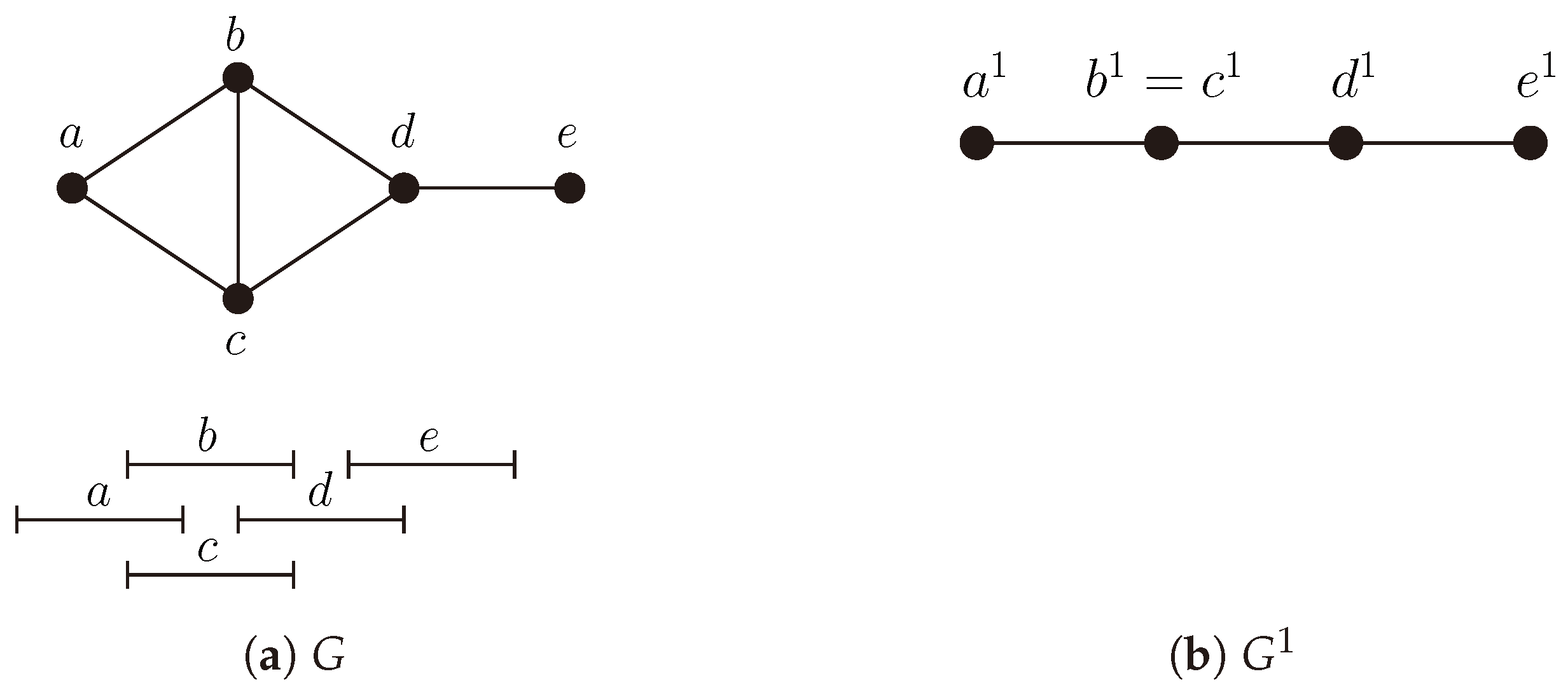
We show a unit interval graph G and its representation through intersections of intervals of length one (see [32]) in Figure 11a. The twin graph of G is in Figure 11b and it is clearly a twin-free graph satisfying$\mathrm{Det}(G^1)=1$. Proposition 3 gives$\mathrm{Det}(G)\in \{n-n^{(1)},n-n^{(1)}+1\}=\{5-4,5-4+1\}=\{1,2\}$. In this case, it is easy to check that$\mathrm{Det}(G)=n-n^{(1)}=1$and both$\{b\}$and$\{c\}$are minimum determining sets of G.

Example 9.

We now show a unit interval graph G and its representation through intersections of intervals of length one in Figure 12a. The twin graph of G (see Figure 12b) is a twin-free graph satisfying$\mathrm{Det}(G^1)=1$. In this case, it is easy to check that $\mathrm{Det}(G)=n-n^{(1)}+1=2$and$\{b,f\}$is an example of minimum determining set of G.

5. Concluding Remarks

In this paper, we provided a lower bound and an upper bound, each of them being tight, of the determining number of general graphs. We also showed that our lower bound is independent from the one obtained in [14]. The main tool that we used is the twin graph, defined in [22] to study the metric dimension of graphs, and which has proven to be also useful for obtaining determining sets and for computing the determining number. Indeed, as an application of our bounds, we computed the exact value of the determining number of cographs. In the case of unit interval graphs, we placed this parameter in an set of two consecutive integers. In both cases, the obtained values depend only on the number of vertices of both graphs G and its twin graph $G^1$.

We think that our bounds could be useful to deal with other graph families (e.g., distance-hereditary graphs or parity graphs) in order to obtain the exact value of their determining numbers, or at least to bound the range of possible values. Actually, we could find other techniques, different from twin deletion, to provide new bounds of the determining number of a graph: addition of vertices or edges, vertex contraction, etc. Furthermore, it could be of interest to apply all those techniques to other types of sets different from determining sets such as dominating sets, cut sets, and independent sets.

References

- Garey, M.R.; Johnson, D.S. Computers and Intractability: A Guide to the Theory of NP-Completeness; W. H. Freeman & Co.: New York, NY, USA, 1979. [Google Scholar]
- Luks, E.M. Isomorphism of Graphs of Bounded Valence Can Be Tested in Polynomial Time. J. Comput. Syst. Sci. 1982, 25, 42–65. [Google Scholar] [CrossRef]
- Boutin, D.L. Identifying Graph Automorphisms Using Determining Sets. Electron. J. Combin. 2006, 13, 78. [Google Scholar]
- Erwin, D.; Harary, F. Destroying automorphisms by fixing nodes. Discret. Math. 2006, 306, 3244–3252. [Google Scholar] [CrossRef]
- Slater, P.J. Leaves of trees. Congr. Numer. 1975, 14, 549–559. [Google Scholar]
- Harary, F.; Melter, R. On the metric dimension of a graph. Ars Combin. 1976, 2, 191–195. [Google Scholar]
- Barragán-Ramírez, G.A.; Estrada-Moreno, A.; Ramírez-Cruz, Y.; Rodríguez-Velázquez, J. The Simultaneous Local Metric Dimension of Graph Families. Symmetry 2017, 9, 132. [Google Scholar] [CrossRef]
- Imran, S.; Siddiqui, M.K.; Imran, M.; Hussain, M.; Bilal, H.M.; Cheema, I.Z.; Tabraiz, A.; Saleem, Z. Computing the Metric Dimension of Gear Graphs. Symmetry 2018, 10, 209. [Google Scholar] [CrossRef]
- Imran, S.; Siddiqui, M.K.; Imran, M.; Hussain, M. On Metric Dimensions of Symmetric Graphs Obtained by Rooted Product. Mathematics 2018, 6, 191. [Google Scholar] [CrossRef]
- Hussain, Z.; Munir, M.; Chaudhary, M.; Kang, S.M. Computing Metric Dimension and Metric Basis of 2D Lattice of Alpha-Boron Nanotubes. Symmetry 2018, 10, 300. [Google Scholar] [CrossRef]
- Liu, J.-B.; Kashif, A.; Rashid, T.; Javaid, M. Fractional Metric Dimension of Generalized Jahangir Graph. Mathematics 2019, 7, 100. [Google Scholar] [CrossRef]
- Wang, J.; Miao, L.; Liu, Y. Characterization of n-Vertex Graphs of Metric Dimension n - 3 by Metric Matrix. Mathematics 2019, 7, 479. [Google Scholar] [CrossRef]
- Cáceres, J.; Garijo, D.; Puertas, M.L.; Seara, C. On the determining number and the metric dimension of graphs. Electron. J. Combin. 2010, 17, 63. [Google Scholar]
- Garijo, D.; González, A.; Márquez, A. The difference between the metric dimension and the determining number of a graph. Appl. Math. Comput. 2014, 249, 487–501. [Google Scholar] [CrossRef]
- Albertson, M.O.; Collins, K.L. Symmetry Breaking in Graphs. Electron. J. Combin. 1996, 3, R18. [Google Scholar]
- Bailey, R.F.; Cameron, P.J. Base size, metric dimension and other invariants of groups and graphs. Bull. Lond. Math. Soc. 2011, 43, 209–242. [Google Scholar] [CrossRef]
- Babai, L. On the complexity of canonical labeling of strongly regular graphs. SIAM J. Comput. 1980, 9, 212–216. [Google Scholar] [CrossRef]
- Blaha, K.D. Minimum Bases for Permutation Groups: The Greedy Approximation. J. Algorithms 1992, 13, 297–306. [Google Scholar] [CrossRef]
- Boutin, D.L. The Determining Number of a Cartesian Product. J. Graph Theory 2009, 61, 77–87. [Google Scholar] [CrossRef]
- Cáceres, J.; Garijo, D.; González, A.; Márquez, A.; Puertas, M.L. The determining number of Kneser graphs. Discret. Math. Theor. Comput. Sci. 2013, 15, 1–14. [Google Scholar]
- Javaid, I.; Azhar, M.N.; Salman, M. Metric Dimension and Determining Number of Cayley Graphs. World Appl. Sci. J. 2012, 18, 1800–1812. [Google Scholar]
- Hernando, C.; Mora, M.; Pelayo, I.M.; Seara, C.; Wood, D.R. Extremal Graph Theory for Metric Dimension and Diameter. Electron. J. Combin. 2010, 17, 30. [Google Scholar] [CrossRef]
- Lerchs, H. On Cliques and Kernels; Technical Report; Department of Computer Science, University of Toronto: Toronto, ON, USA, 1971. [Google Scholar]
- Seinsche, D. On a property of the class of n-colorable graphs. J. Comb. Theory (B) 1974, 16, 191–193. [Google Scholar] [CrossRef]
- Sumner, D.P. Dacey graphs. J. Austral. Math. Soc. 1974, 18, 492–502. [Google Scholar] [CrossRef]
- Jung, H.A. On a class of posets and the corresponding comparability graphs. J. Comb. Theory (B) 1978, 24, 125–133. [Google Scholar] [CrossRef]
- Corneil, D.G.; Lerchs, H.; Stewart-Burlingham, L. Complement reducible graphs. Discret. Appl. Math. 1981, 3, 163–174. [Google Scholar] [CrossRef]
- Corneil, D.G.; Perl, Y.; Stewart, L. Cographs: recognition, application and algorithms. Congr. Numer. 1984, 43, 249–258. [Google Scholar]
- Randerath, B.; Schiermeyer, I. Vertex Colouring and Forbidden Subgraphs—A Survey. Graphs Combin. 2004, 20, 1–40. [Google Scholar] [CrossRef]
- Fishburn, P.C. Interval graphs and interval orders. Discret. Math. 1985, 55, 135–149. [Google Scholar] [CrossRef]
- Roberts, F.S. Indifference graphs. In Proof Techniques in Graph Theory (Proceedings of the Second Ann Arbor Graph Theory Conference, Ann Arbor, MI, USA, 1968); Academic Press: New York, NY, USA, 1969; pp. 139–146. [Google Scholar]
- Hanlon, P. Counting Interval Graphs. Trans. Amer. Math. Soc. 1982, 272, 383–426. [Google Scholar] [CrossRef]
Figure 1.
The Petersen graph.
Figure 2.
A graph G and its twin graph .
Figure 3.
is a plenty twin set but it is not a determining set.
Figure 4.
.
Figure 5.
Figure 6.
Figure 7.
is not necessarily a twin-free graph.
Figure 8.
The sequence of twin graphs obtained from G.
Figure 9.
Figure 10.
A cograph G and its twin graph .
Figure 11.
A unit interval G and its twin graph .
Figure 12.
© 2019 by the authors. Licensee MDPI, Basel, Switzerland. This article is an open access article distributed under the terms and conditions of the Creative Commons Attribution (CC BY) license (http://creativecommons.org/licenses/by/4.0/).
Share and Cite
MDPI and ACS Style
González, A.; Puertas, M.L. Removing Twins in Graphs to Break Symmetries. Mathematics 2019, 7, 1111. https://doi.org/10.3390/math7111111
AMA Style
González A, Puertas ML. Removing Twins in Graphs to Break Symmetries. Mathematics. 2019; 7(11):1111. https://doi.org/10.3390/math7111111
Chicago/Turabian StyleGonzález, Antonio, and María Luz Puertas. 2019. "Removing Twins in Graphs to Break Symmetries" Mathematics 7, no. 11: 1111. https://doi.org/10.3390/math7111111
Note that from the first issue of 2016, this journal uses article numbers instead of page numbers. See further details here.