Numerically Efficient Methods for Variational Fractional Wave Equations: An Explicit Four-Step Scheme

Abstract

In this work, we investigate numerically a one-dimensional wave equation in generalized form. The system considers the presence of constant damping and functional anomalous diffusion of the Riesz type. Reaction terms are also considered, in such way that the mathematical model can be presented in variational form when damping is not present. As opposed to previous efforts available in the literature, the reaction terms are not only functions of the solution. Instead, we consider the presence of smooth functions that depend on fractional derivatives of the solution function. Using a finite-difference approach, we propose a numerical scheme to approximate the solutions of the fractional wave equation. Along with this integrator, we propose discrete forms of the local and the total energy operators. In a first stage, we show rigorously that the energy properties of the continuous system are mimicked by our discrete methodology. In particular, we prove that the discrete system is dissipative (respectively, conservative) when damping is present (respectively, absent), in agreement with the continuous model. The theoretical numerical analysis of this system is more complicated in light of the presence of the functional form of the anomalous diffusion. To solve this problem, some novel technical lemmas are proved and used to establish the stability and the quadratic convergence of the scheme. Finally, we provide some computer simulations to show the capability of the scheme to conserve/dissipate the energy. Various fractional problems with functional forms of the anomalous diffusion of the solution are considered to that effect.

1. Introduction

The design of energy-preserving methods for physical systems has been a fruitful avenue of research in the last decades. Historically, the problem of designing energy-conserving methods may date back to the decade of the 1970s [1,2]. However, L. Vázquez and coauthors were probably the first researchers who pointed out the physical and mathematical significance of designing this type of schemes [3]. Various seminal papers by Vázquez and his coworkers were published in the 1990s, including various energy-conserving numerical schemes to solve partial differential equations such as the Schrödinger equation [4], the sine-Gordon equation [5,6], the Klein–Gordon equations [7], and even systems consisting of ordinary differential equations [8]. In those papers, the authors established thoroughly the capability of their schemes to preserve the energy properties of the continuous problem. Moreover, they employed a discrete form of the energy method to establish rigorously the stability and the convergence properties of the schemes. After the publication of those works, the investigation on energy-conserving schemes became a highly transited route of investigation, and many interesting articles were proposed in the specialized literature. As examples, some energy-preserving methods have been proposed to simulate the nonlinear dynamics of three-dimensional beams undergoing finite rotations [9], to approximate the kinematics of geometrically exact rods [10] and to design algorithms for frictionless dynamic contact problems [11].

After those seminal works by Vázquez and coauthors, the investigation on energy-preserving schemes became a vast area of research. However, those papers by D. Furihata and collaborators published at the beginning of the millennium became a landmark in the area [12,13]. In particular, they contributed to the state of the art by reviewing various existing methods for hyperbolic partial differential equations, which conserved or dissipated the energy of the systems [14,15]. Those works would eventually pave the road to the birth of the discrete variational derivative method, which is a helpful tool to construct finite-difference schemes resembling he variational properties of continuous models [16]. Various works have been published in that area, including studies for the simulation of nonlinear partial differential equations with variable coefficients [17], the solution of nonlinear systems based on the use of discrete differential forms [18], the investigation of numerical schemes using average-difference approaches [19], the two-dimensional vorticity equation [20], the solution of Hamilton’s equation using variational principles [21], and the investigation of coupled partial differential equations through an alternating form of the discrete variational derivative method [22], among other interesting works. Needless to mention that this approach has been extended to consider different methods, including finite elements [23], finite volumes, and Galerkin techniques [24,25,26].

On the other hand, fractional derivatives have been introduced to mathematical models in order to provide more realistic descriptions of the physical phenomena. For instance, many fractional systems have been obtained as the continuous limit of discrete systems of particles with long-range interactions [27], and fractional derivatives have been successfully used in the theory of viscoelasticity [28], the theory of thermoelasticity [29], financial problems under a continuous time frame [30], self-similar protein dynamics [31] and quantum mechanics [32]. As expected, the complexity of fractional problems is considerably higher than that of integer-order models, whence the need to design reliable numerical techniques to approximate the solutions is pragmatically justified [33,34]. In this direction, the literature reports on various methods to approximate the solutions of fractional systems. For example, some numerical methods have been proposed to solve fractional partial differential equations using fractional centered differences [35,36,37], the time-fractional diffusion equation [38], the fractional Schrödinger equation in multiple spatial dimensions [39], the nonlinear fractional Korteweg–de Vries–Burgers equation [40], and the fractional FitzHugh–Nagumo monodomain models [41], among other examples [42,43,44,45].

Despite the tremendous amount of works in both variational and fractional schemes, sufficiently general models which include reaction functions in terms of fractional derivatives have not been investigated thoroughly yet. The reason is obviously the high level of difficulty to analyze the efficiency of the corresponding numerical methods. This is partly due to the lack of strong analytical results which may help in the theoretical studies of the stability and the convergence of the methodologies. To alleviate this situation, we investigate a general wave equation which extends various particular variational models from physics, including the Klein–Gordon and continuous forms of the Fermi–Pasta–Ulam–Tsingou arrays [46]. We exhibit the variational structure of the mathematical model proposed, and propose a finite-difference method to solve it. Together with the discrete forms of the equation of motion, we introduce a discretization of the local and total energies of the system, and we show that the same variational structure of the continuous problem is preserved by the discrete system. In that sense, our numerical scheme is a structure-preserving methodology [47]. In turn, the theoretical investigation of the stability and the quadratic convergence of the scheme requires novel analytical results to estimate the reaction functions that depend on the fractional derivatives, along with a discrete Gronwall inequality. Some illustrative simulations are provided to show the capability of the scheme to conserve or dissipate the energy. For the sake of computational efficiency and speed, we implemented the numerical method in a Fortran 95. However, we must point out that the algorithm can be implemented in any scientific computer language, including C++ or Matlab.

This work is organized as follows. In Section 2, we present the fractional partial differential equation of interest. The model is an extension of some continuous generalizations of the classical wave equation with constant damping and fractional diffusion. We propose an energy density function associated to our model. Moreover, we prove therein that the total energy of the system is conserved or dissipated, depending on whether damping is absent or present. Section 3 introduces the discrete nomenclature employed throughout this work, and presents the finite-difference scheme to approximate the solutions of the mathematical model. Discrete forms of the local and total energy are presented therein, and we establish a discrete analog of the theorem on the conservation/dissipation of energy of the continuous model. As expected, the boundedness of the numerical solutions is established under the same conditions of the continuous-case scenario. In turn, the purpose of Section 4 is to establish the main numerical features of our discrete model. Some illustrative simulations are shown in Section 5. We close this work with some concluding remarks.

2. Preliminaries

We let $I_n=\{1,\dots ,n\}$ and ${\overline{I}}_n=I_n\cup \left\{0\right\}$, for each $n\in \mathbb{N}$. Throughout, we let $\gamma \in {\mathbb{R}}^{+}\cup \left\{0\right\}$ represent physically a constant damping coefficient. Let a and b be real numbers such that $a<b$, and let $B=(a,b)\subseteq \mathbb{R}$ and $\mathsf{\Omega }=B\times (0,T)\subseteq {\mathbb{R}}^2$. We employ the symbols $\partial B$, $\overline{B}$ and $\overline{\mathsf{\Omega }}$ to denote, respectively, the boundary of B, and the closures of B and $\mathsf{\Omega }$ with respect to the standard topology of ${\mathbb{R}}^2$. In the following, we let $u:\overline{\mathsf{\Omega }}\to \mathbb{R}$ be a function, and extend the definition of u by letting $u(x,t)=0$, for each $(x,t)\in (\mathbb{R}\backslash \overline{B})\times [0,T]$. Throughout this manuscript, we let $\mathsf{\Gamma }$ denote the usual Gamma function that generalizes factorials.

Definition 1.

Let $L_{x,2}\left(\overline{\mathsf{\Omega }}\right)$ denote the set of all functions $f:\overline{\mathsf{\Omega }}\to \mathbb{R}$ such that $f(·,t)\in L_2\left(\overline{B}\right)$ for each $t\in [0,T]$. Moreover, for each pair $f,g\in L_{x,2}\left(\overline{\mathsf{\Omega }}\right)$, the inner product of f and g is the function of t defined by

$${〈f,g〉}_x={\int }_{\overline{B}}f(x,t)g(x,t)dx,\forall t\in [0,T].$$

(1)

In turn, the Euclidean norm of $f\in L_{x,2}\left(\overline{\mathsf{\Omega }}\right)$ is the function of t defined by ${\parallel f\parallel }_{x,2}=\sqrt{{〈f,f〉}_x}$. In general, if $1\le q<\infty$, then $L_{x,q}\left(\overline{\mathsf{\Omega }}\right)$ represents the set of all functions $f:\overline{\mathsf{\Omega }}\to \mathbb{R}$ such that $f(·,t)\in L_q\left(\overline{B}\right)$, for each $t\in [0,T]$. For each such function f, we define its norm as the function of t given by

$${\parallel f\parallel }_{x,q}={\left({\int }_{\overline{B}}{\left|f(x,t)\right|}^{q}dx\right)}^{1/q},\forall t\in [0,T].$$

(2)

Definition 2.

Let $f:\mathbb{R}\to \mathbb{R}$ be a function, and let $n\in \mathbb{N}\cup \left\{0\right\}$ and $\alpha \in \mathbb{R}$ satisfy $n-1<\alpha <n$. The Riesz fractional derivative of f of order α at $x\in \mathbb{R}$ is defined (when it exists) as

$$\frac{d^{\alpha }f\left(x\right)}{{d\left|x\right|}^{\alpha }}=\frac{-1}{2cos\left(\frac{\pi \alpha }{2}\right)\mathsf{\Gamma }(n-\alpha )}\frac{d^n}{d{x}^n}{\int }_{-\infty }^{\infty }\frac{f\left(\xi \right)d\xi }{{|x-\xi |}^{\alpha +1-n}}.$$

(3)

Definition 3.

Let $\alpha \in \mathbb{R}$ and $n\in \mathbb{N}$ be such that $n-1<\alpha <n$. When it exists, the Riesz space-fractional partial derivative of the function $u:\overline{\mathsf{\Omega }}\to \mathbb{R}$ of order α with respect to x at the point $(x,t)$ is defined by

$$\frac{{\partial }^{\alpha }u(x,t)}{{\partial \left|x\right|}^{\alpha }}=\frac{-1}{2cos\left(\frac{\pi \alpha }{2}\right)\mathsf{\Gamma }(n-\alpha )}\frac{{\partial }^n}{\partial x^n}{\int }_{-\infty }^{\infty }\frac{u(\xi ,t)d\xi }{{|x-\xi |}^{\alpha +1-n}},\forall (x,t)\in \mathsf{\Omega }.$$

(4)

For the sake of convenience, if $n\in \{1,2\}$, then we let the Riesz partial derivative of u of order n to be equal to the usual partial derivative of u of order n with respect to x.

Riesz fractional partial derivatives are self-adjoint and non-positive operators [48]. It follows that their additive inverses are self-adjoint and nonnegative, which implies, in turn, that they possess square-root operators [49]. This means in particular that, if $\alpha \in (1,2]$ and $u,v:\overline{\mathsf{\Omega }}\to \mathbb{R}$, then

$$〈-\frac{{\partial }^{\alpha }u}{{\partial \left|x\right|}^{\alpha }},v〉=〈u,-\frac{{\partial }^{\alpha }v}{{\partial \left|x\right|}^{\alpha }}〉=〈\frac{{\partial }^{\alpha /2}u}{{\partial \left|x\right|}^{\alpha /2}},\frac{{\partial }^{\alpha /2}v}{{\partial \left|x\right|}^{\alpha /2}}〉,\forall t\in [0,T].$$

(5)

For the remainder of this manuscript, we let $\varphi ,\psi :\overline{\mathsf{\Omega }}\to \mathbb{R}$ be sufficiently smooth functions vanishing at the boundary of $\mathsf{\Omega }$, and let $p\in \mathbb{N}$. Suppose that ${\alpha }_1,\dots ,{\alpha }_p\in (1,2]$ are constants, and let $G,G_1,G_2,\dots ,G_p:\mathbb{R}\to \mathbb{R}$ be smooth functions. In particular, we assume that $G=G\left(v\right)$ and $G_j=G_j\left(v\right)$, for each $v\in \mathbb{R}$ and $j\in I_p$. With these conventions, the problem under investigation in this work is the initial-value problem with homogeneous Dirichlet boundary data

$$\begin{array}{c}{\displaystyle \frac{{\partial }^{2}u(x,t)}{\partial t^2}+\gamma \frac{\partial u(x,t)}{\partial t}+\frac{dG\left(u\right(x,t\left)\right)}{dv}-\sum _{j=1}^p\frac{{\partial }^{{\alpha }_j/2}}{{\partial \left|x\right|}^{{\alpha }_j/2}}\frac{d{G}_j}{dv}\left(\frac{{\partial }^{{\alpha }_j/2}u(x,t)}{{\partial \left|x\right|}^{{\alpha }_j/2}}\right)=0,\forall (x,t)\in \mathsf{\Omega },}\\ \mathrm{such}\mathrm{that}\left\{\begin{array}{cc}u(x,0)=\varphi \left(x\right),\hfill & \forall x\in B,\hfill \\ {\displaystyle \frac{\partial u(x,0)}{\partial t}=\psi \left(x\right),}\hfill & \forall x\in B,\hfill \\ u(x,t)=0,\hfill & \forall (x,t)\in \partial B\times [0,T].\hfill \end{array}\right.\end{array}$$

(6)

Definition 4.

Let u be a function satisfying the initial-boundary-value problem in Equation (6). We define the local energy density of the undamped system as the function

$$\mathcal{H}(x,t)=\frac{1}{2}{\left(\frac{\partial u(x,t)}{\partial t}\right)}^2+G\left(u(x,t)\right)+\sum _{j=1}^p{G}_j\left(\frac{{\partial }_x^{{\alpha }_j/2}u(x,t)}{{\partial \left|x\right|}^{{\alpha }_j/2}}\right),\forall (x,t)\in \mathsf{\Omega }.$$

(7)

In turn, the total energy at the time $t\in (0,T)$ is given by

$$\mathcal{E}\left(t\right)={\int }_{\mathbb{R}}\mathcal{H}(x,t)dx=\frac{1}{2}{∥\frac{\partial u}{\partial t}∥}_{x,2}^2+{\int }_{\mathbb{R}}G\left(u(x,t)\right)dx+\sum _{j=1}^p{\int }_{\mathbb{R}}{G}_j\left(\frac{{\partial }_x^{{\alpha }_j/2}u(x,t)}{{\partial \left|x\right|}^{{\alpha }_j/2}}\right)dx.$$

(8)

Theorem 1 (Dissipation of energy).

If u satisfies Equation (6), then ${\mathcal{E}}^{\prime }\left(t\right)=-\gamma {\parallel u_t\parallel }_{x,2}^2$, where $u_t=u_t(x,t)$ is the partial derivative of u with respect to t at $(x,t)$. The system in Equation (6) is conservative if $\gamma =0$. In general,

$$\mathcal{E}\left(t\right)=\mathcal{E}\left(0\right)-\gamma {\int }_0^t{\parallel u_t\parallel }_{x,2}^{2}dt,\forall t\in (0,T).$$

(9)

Proof. 

We take the derivative of each of the three terms at the right-hand side of Equation (8). For the third term, we use the square-root properties of fractional derivatives along with the chain rule. The first two terms only require the use of the chain rule. In such way, we readily obtain

$$\begin{array}{cc}\hfill \frac{1}{2}\frac{d}{dt}{∥\frac{\partial u}{\partial t}∥}_{x,2}^2& ={〈\frac{{\partial }^{2}u}{\partial t^2},\frac{\partial u}{\partial t}〉}_x,\hfill \end{array}$$

(10)

$$\begin{array}{cc}\hfill \frac{d}{dt}{\int }_{\mathbb{R}}G\left(u(x,t)\right)dx& ={〈\frac{dG\left(u\right)}{dv},\frac{\partial u}{\partial t}〉}_x\hfill \end{array}$$

(11)

and

$$\begin{array}{cc}\hfill \frac{d}{dt}{\int }_{\mathbb{R}}{G}_j\left(\frac{{\partial }_x^{{\alpha }_j/2}u(x,t)}{{\partial \left|x\right|}^{{\alpha }_j/2}}\right)dx& ={〈\frac{d{G}_j}{dv}\left(\frac{{\partial }_x^{{\alpha }_j/2}u}{{\partial \left|x\right|}^{{\alpha }_j/2}}\right),\frac{{\partial }^{{\alpha }_j/2}}{{\partial \left|x\right|}^{{\alpha }_j/2}}\frac{\partial u}{\partial t}〉}_x\hfill \\ \hfill & =-{〈\frac{{\partial }^{{\alpha }_j/2}}{{\partial \left|x\right|}^{{\alpha }_j/2}}\frac{d{G}_j}{dv}\left(\frac{{\partial }_x^{{\alpha }_j/2}u}{{\partial \left|x\right|}^{{\alpha }_j/2}}\right),\frac{\partial u}{\partial t}〉}_x,\hfill \end{array}$$

(12)

for each $t\in (0,T)$ and $j\in I_p$. Taking the derivative with respect to t on both sides of Equation (8), exchanging the derivative and integral operators, using then the identities above and regrouping, we reach

$$\begin{array}{cc}\hfill {\mathcal{E}}^{\prime }\left(t\right)& =〈\frac{{\partial }^{2}u}{\partial t^2}+\frac{dG\left(u\right)}{dv}-\sum _{j=1}^p\frac{{\partial }^{{\alpha }_j/2}}{{\partial \left|x\right|}^{{\alpha }_j/2}}\frac{d{G}_j}{dv}\left(\frac{{\partial }^{{\alpha }_j/2}u}{{\partial \left|x\right|}^{{\alpha }_j/2}}\right),\frac{\partial u}{\partial t}〉=-\gamma {∥\frac{\partial u}{\partial t}∥}_{x,2}^2,\forall t\in (0,T),\hfill \end{array}$$

(13)

as desired. It is obvious now that the system is conservative if $\gamma =0$. Moreover, the identity in Equation (9) is also an immediate consequence of the fact that ${\mathcal{E}}^{\prime }\left(t\right)=-\gamma {\parallel u_t\parallel }_{x,2}^2$, which is obtained by integrating both sides of this equation over $(0,t)$. □

Corollary 1

(Energy positivity). Suppose that G, $G_1$, $G_2$, …, $G_p$ are all nonnegative functions. Then, $\mathcal{E}$ is likewise nonnegative in $(0,T)$ and, moreover,

$$\mathcal{E}\left(t\right)=\frac{1}{2}{∥\frac{\partial u}{\partial t}∥}_{x,2}^2+{\parallel G\left(u\right)\parallel }_{x,1}+\sum _{j=1}^p{∥G_j\left(\frac{{\partial }_x^{{\alpha }_j/2}u}{{\partial \left|x\right|}^{{\alpha }_j/2}}\right)∥}_{x,1},\forall t\in (0,T).$$

(14)

Corollary 2 (Boundedness).

If G, $G_1$, $G_2$, …, $G_p$ are nonnegative functions, then there exists a constant $C\ge 0$ that depends only on ϕ and ψ, such that each of the terms at the right-hand side of Equation (14) is uniformly bounded by C, for all $t\ge 0$.

Proof. 

Using the hypotheses of this result and Theorem 1, we readily obtain the next inequalities, valid for all $t\ge 0$:

$$\begin{array}{cc}\hfill & max\left\{{∥\frac{\partial u}{\partial t}∥}_{x,2}^2,{∥G\left(u\right)∥}_{x,1}\right\}\vee max\left\{{∥G_j\left(\frac{{\partial }_x^{{\alpha }_j/2}u}{{\partial \left|x\right|}^{{\alpha }_j/2}}\right)∥}_{x,1}:j\in I_p\right\}\hfill \\ \hfill & \le 2\mathcal{E}\left(t\right)\le 2\mathcal{E}\left(0\right)-2\gamma {\int }_0^t{\parallel u_t\parallel }_{x,2}^{2}dt\le 2\mathcal{E}\left(0\right).\hfill \end{array}$$

(15)

Let C be the right-hand side of his chain of inequalities. Note that

$$C={\parallel \psi \parallel }_{x,2}^2+2{\parallel G\left(\varphi \right)\parallel }_{x,1}+2\sum _{j=1}^p{∥G_j\left(\frac{{\partial }_x^{{\alpha }_j/2}\varphi }{{\partial \left|x\right|}^{{\alpha }_j/2}}\right)∥}_{x,1},$$

(16)

whence the conclusion of this proposition readily follows. □

In the following examples, we provide some fractional generalizations of well-known variational systems from the physical sciences. The systems considered therein will be particular forms of the hyperbolic partial differential equation in Equation (6).

Example 1.

In the following examples, we assume that $\gamma =0$ and $p=1$.

(a) 

Suppose that $G\left(v\right)=1-cos\left(v\right)$ and $G_1\left(v\right)=\frac{1}{2}{v}^2$, for each $v\in \mathbb{R}$. Then, the resulting partial differential equation in Equation (6) is the fractional sine-Gordon equation, which is a well-known physical model that appears in relativistic quantum mechanics.

(b) 

The fractional form of the nonlinear Klein–Gordon equation is obtained from the partial differential equation of Equation (6) when $G\left(v\right)=\frac{1}{2!}{v}^2-\frac{1}{4!}{v}^4$ for each $v\in \mathbb{R}$, and $G_1$ is as in(a). The Klein–Gordon equation is also a useful model in relativistic quantum mechanics and particle physics.

(c) 

If $G_1$ is as in(a)and $G\left(v\right)=1-\frac{1}{3}cosv-\frac{1}{6}cos\left(2v\right)$ for each $v\in \mathbb{R}$, then the partial differential equation resulting in Equation (6) is the fractional double sine-Gordon equation.

(d) 

Let $ϵ>0$ and $p\in \mathbb{N}$ satisfy $p\ge 3$. If $G\equiv 0$ and $G_1\left(v\right)=\frac{1}{2}{v}^2+ϵv^p$ for each $v\in \mathbb{R}$, then the resulting equation is a fractional and continuous extension of the Fermi–Pasta–Ulam–Tsingou chains [50,51].

Obviously, all the models in this example reduce to their well-known integer-order systems when $\alpha =2$.

3. Numerical Method

In this section, we provide the discrete nomenclature used for the remainder of the present work, and introduce the finite-difference method to solve Equation (6) along with a discrete form of the Hamiltonian in Equation (7). Moreover, we show that a discrete form of Theorem 1 is satisfied in the discrete-case scenario. To that end, we consider a regular partition of the interval $\overline{B}$, consisting of $M\in \mathbb{N}$ subintervals. The norm of the partition is represented by $h=(b-a)/M$, and the nodes are defined by $x_m=a+mh$, for each $m\in {\overline{I}}_M$. Similarly, fix a uniform partition of $[0,T]$ consisting of $N\in \mathbb{N}$ subintervals, and let $\tau$ be the respective partition norm. For each $n\in {\overline{I}}_N$, agree that $t_n=n\tau$.

Throughout, we fix $J=I_{M-1}\times I_{N-2}$ and $\overline{J}={\overline{I}}_M\times {\overline{I}}_N$. Let us use ${\mathcal{R}}_h$ to represent the spatial grid $\{x_m:m\in {\overline{I}}_M\}$, and ${\mathcal{V}}_h$ to represent the real vector space of all functions $f:{\mathcal{R}}_h\to \mathbb{R}$, such that $f\left(x_0\right)=f\left(x_M\right)=0$. For simplicity, if $f\in {\mathcal{V}}_h$ and $m\in {\overline{I}}_M$, then we set $f_m=f\left(x_m\right)$. In this work, unless we mention something different, we use the symbol $U_m^n$ to represent an approximation to the exact value of the solution u of Equation (6) at the point $(x_m,t_n)$, for each $(m,n)\in \overline{J}$. Moreover, let

$$U^n={\left(U_m^n\right)}_{m\in {\overline{I}}_M}=(U_0^n,U_1^n,\dots ,U_M^n)\in {\mathcal{V}}_h,\forall n\in {\overline{I}}_N.$$

(17)

Definition 5.

Define the inner product$\langle ·,·\rangle :{\mathcal{V}}_h\times {\mathcal{V}}_h\to \mathbb{R}$ and the norm ${\parallel ·\parallel }_p:{\mathcal{V}}_h\to \mathbb{R}$ by

$$\langle U,V\rangle =h\sum _{m\in {\overline{I}}_M}{U}_m{V}_m,{\parallel U\parallel }_p={\left[h\sum _{m\in {\overline{I}}_M}{\left|U_m\right|}^p\right]}^{1/p},\forall U,V\in {\mathcal{V}}_h.$$

(18)

The Euclidean norm induced by $\langle ·,·\rangle$ is denoted by ${\parallel ·\parallel }_2$, and ${\parallel ·\parallel }_{\infty }:{\mathcal{V}}_h\to \mathbb{R}$ is the usual infinity norm in ${\mathcal{V}}_h$, which is defined as ${\parallel U\parallel }_{\infty }=max\left\{\right|U_m|:m\in {\overline{I}}_M\}$, for each $U\in {\mathcal{V}}_h$.

Definition 6.

Let ${\left(U^n\right)}_{n\in {\overline{I}}_N}\subseteq {\mathcal{V}}_h$. We introduce the linear difference operators on ${\mathcal{V}}_h$ defined by

$$\begin{array}{cc}\hfill {\delta }_t{U}_m^{n+\frac{1}{2}}& =\frac{U_m^{n+1}-U_m^n}{\tau },\forall U\in {\mathcal{V}}_h,\forall (m,n)\in J,\hfill \end{array}$$

(19)

$$\begin{array}{cc}\hfill {\mu }_t{U}_m^{n+\frac{1}{2}}& =\frac{U_m^{n+1}+U_m^n}{2},\forall U\in {\mathcal{V}}_h,\forall (m,n)\in J,\hfill \end{array}$$

(20)

$$\begin{array}{cc}\hfill {\delta }_t^{\left(2\right)}{U}_m^n& =\frac{U_m^{n+1}-2U_m^n+U_m^{n-1}}{{\tau }^2},\forall U\in {\mathcal{V}}_h,\forall (m,n)\in J.\hfill \end{array}$$

(21)

For convenience, we let $t_{n+\frac{1}{2}}=(n+\frac{1}{2})\tau$, for each $n\in {\overline{I}}_{N-1}$. If $U:\overline{\mathsf{\Omega }}\to \mathbb{R}$ is a sufficiently smooth function then the value Equation (19) is a second-order consistent approximation for the partial derivative of U with respect to t at the point $(x_m,t_{n+\frac{1}{2}})$. In addition, the quantity in Equation (20) is a second-order approximation to the value of U at the same point. In turn, Equation (21) approximates the second-order partial derivative of U with respect to t at $(x_m,t_n)$ with second order of consistency. It is easy to see that

$${\widehat{\delta }}_t^{\left(2\right)}{U}_m^{n+\frac{1}{2}}={\delta }_t^{\left(2\right)}{\mu }_t{U}_m^{n+\frac{1}{2}}=\frac{U_m^{n+2}-U_m^{n+1}-U_m^n+U_m^{n-1}}{2{\tau }^2}$$

(22)

approximates consistently the second-order derivative of U with respect to t at the point $(x_m,t_{n+\frac{1}{2}})$ with a quadratic order of consistency.

Definition 7.

For any function $f:\mathbb{R}\to \mathbb{R}$, $h>0$ and $\alpha >-1$, we define the fractional centered difference of order α of f at the point x as

$${\mathsf{\Delta }}_h^{\alpha }f\left(x\right)=\sum _{k=-\infty }^{\infty }{g}_k^{\left(\alpha \right)}f(x-kh),\forall x\in \mathbb{R},$$

(23)

where

$$g_k^{\left(\alpha \right)}=\frac{{(-1)}^k\mathsf{\Gamma }(\alpha +1)}{\mathsf{\Gamma }(\frac{\alpha }{2}-k+1)\mathsf{\Gamma }(\frac{\alpha }{2}+k+1)},\forall k\in \mathbb{N}\cup \left\{0\right\}.$$

(24)

Lemma 1

(Wang et al. [52]). Let $0<\alpha \le 2$ and $\alpha \ne 1$.

(a) 

The coefficients ${\left(g_k^{\left(\alpha \right)}\right)}_{k=-\infty }^{\infty }$ satisfy

$$g_0^{\left(\alpha \right)}=\frac{\mathsf{\Gamma }(\alpha +1)}{\mathsf{\Gamma }{(\alpha /2+1)}^2},g_{k+1}^{\left(\alpha \right)}=\left(1-\frac{\alpha +1}{\alpha /2+k+1}\right)g_k,\forall k\in \mathbb{N}\cup \left\{0\right\}.$$

(25)

(b) 

$g_0^{\left(\alpha \right)}\ge 0$.

(c) 

$g_k^{\left(\alpha \right)}=g_{-k}^{\left(\alpha \right)}<0$ for all $k\ge 1$, and

(d) 

${\displaystyle \sum _{k=-\infty }^{\infty }{g}_k^{\left(\alpha \right)}=0}$. It follows that ${\displaystyle g_0^{\left(\alpha \right)}=-\sum _{\begin{array}{c}k=-\infty \\ k\ne 0\end{array}}^{\infty }{g}_k^{\left(\alpha \right)}}$.

When $\alpha \in (0,1)\cup (1,2]$, $h>0$ and $f\in {\mathcal{C}}^5\left(\mathbb{R}\right)$ has its derivatives up to order five which belong to $L^1\left(\mathbb{R}\right)$, then the following consistency property holds true (see [52]):

$$-\frac{1}{h^{\alpha }}{\mathsf{\Delta }}_h^{\alpha }f\left(x\right)=\frac{d^{\alpha }f\left(x\right)}{{d\left|x\right|}^{\alpha }}+\mathcal{O}\left(h^2\right),\forall x\in \mathbb{R}.$$

(26)

Definition 8.

Let $U\in {\mathcal{V}}_h$ and $\alpha \in (0,2]$. If $m=0,M$, then we convey that ${\delta }_x^{\left(\alpha \right)}{U}_m=0$. Otherwise, we let

$${\delta }_x^{\left(\alpha \right)}{U}_m=\left\{\begin{array}{cc}{\displaystyle \frac{U_{m+1}-2U_m+U_{m-1}}{h^2},}\hfill & if \alpha =2,\hfill \\ {\displaystyle -\frac{1}{h^{\alpha }}\sum _{k=0}^M{g}_{m-k}^{\left(\alpha \right)}{U}_k,}\hfill & if \alpha \in (0,1)\cup (1,2).\hfill \end{array}\right.$$

(27)

Lemma 2

(Macías-Díaz [53]). If $\alpha \in (1,2]$ then $\langle -{\delta }_x^{\left(\alpha \right)}U,V\rangle =\langle {\delta }_x^{(\alpha /2)}U,{\delta }_x^{(\alpha /2)}V\rangle$, for any $U,V\in {\mathcal{V}}_h$. Moreover, if $\alpha \in (1,2]$ and $g_h^{\left(\alpha \right)}=2g_0^{\left(\alpha \right)}{h}^{1-\alpha }$, then

(a) 

$\parallel {\delta }_x^{(\alpha /2)}{V\parallel }_2^2\le g_h^{\left(\alpha \right)}{\parallel V\parallel }_2^2$, for each $V\in {\mathcal{V}}_h$, and

(b) 

$\parallel {\delta }_x^{\left(\alpha \right)}{V\parallel }_2^2\le (g_h^{\left(\alpha \right)}{\parallel V\parallel }_2{)}^2$, for each $V\in {\mathcal{V}}_h$.

Definition 9.

Let ${\left(U^n\right)}_{n\in {\overline{I}}_N}\subseteq {\mathcal{V}}_h$, and suppose that $G:{\mathbb{R}}^{p+2}\to \mathbb{R}$ is a continuously differentiable function. We introduce the nonlinear difference operators ${\delta }_{U}G$ and ${\delta }_U{G}_j$ defined on ${\mathcal{V}}_h$ by the formulas

$${\delta }_{U}G\left(U_m^{n+\frac{1}{2}}\right)=\left\{\begin{array}{cc}{\displaystyle \frac{G\left(U_m^{n+1}\right)-G\left(U_m^n\right)}{U_m^{n+1}-U_m^n},}\hfill & \mathit{if}{U}_m^{n+1}\ne U_m^n,\hfill \\ G^{\prime }\left(U_m^{n+\frac{1}{2}}\right),\hfill & \mathit{if}{U}_m^{n+1}=U_m^n,\hfill \end{array}\right.$$

(28)

and

$${\delta }_{{\delta }_x^{({\alpha }_j/2)}U}{G}_j\left(U_m^{n+\frac{1}{2}}\right)=\left\{\begin{array}{cc}{\displaystyle \frac{G_j\left({\delta }_x^{({\alpha }_j/2)}{U}_m^{n+1}\right)-G\left({\delta }_x^{({\alpha }_j/2)}{U}_m^n\right)}{{\delta }_x^{({\alpha }_j/2)}{U}_m^{n+1}-{\delta }_x^{({\alpha }_j/2)}{U}_m^n},}\hfill & \mathit{if}{\delta }_x^{({\alpha }_j/2)}{U}_m^{n+1}\ne {\delta }_x^{({\alpha }_j/2)}{U}_m^n,\hfill \\ G^{\prime }\left({\displaystyle \frac{{\partial }^{{\alpha }_j/2}{U}_m^{n+\frac{1}{2}}}{{\partial \left|x\right|}^{{\alpha }_j/2}}}\right),\hfill & \mathit{if}{\delta }_x^{({\alpha }_j/2)}{U}_m^{n+1}={\delta }_x^{({\alpha }_j/2)}{U}_m^n,\hfill \end{array}\right.$$

(29)

for each $(m,n)\in J$ and $j\in I_p$. In addition, for any function $F:\mathbb{R}\to \mathbb{R}$, we employ $F\left(U^n\right)$ to represent the vector $(F\left(U_0^n\right),F\left(U_1^n\right),\dots ,F\left(U_M^n\right))\in {\mathcal{V}}_h$. Moreover, we use the symbol “1” to represent both the multiplicative identity of $\mathbb{R}$ and the $(M+1)$-dimensional vector all of whose components are equal to 1.

At this stage of our discussion, the nomenclature introduced thus far suffices to provide the full finite-difference discretization of the model in Equation (6). The numerical method proposed in this manuscript is given by the discrete system

$$\begin{array}{c}{\displaystyle {\widehat{\delta }}_t^{\left(2\right)}{U}_m^{n+\frac{1}{2}}+\gamma {\delta }_t{U}_m^{n+\frac{1}{2}}+{\delta }_{U}G\left(U_m^{n+\frac{1}{2}}\right)-\sum _{j=1}^p{\delta }_x^{({\alpha }_j/2)}\left[{\delta }_{{\delta }_x^{({\alpha }_j/2)}U}{G}_j\left(U_m^{n+\frac{1}{2}}\right)\right]=0,\forall (m,n)\in J,}\\ \mathrm{such}\mathrm{that}\left\{\begin{array}{cc}{U}_m^0={\varphi }_U\left(x_m\right),\hfill & \forall m\in I_{M-1},\hfill \\ U_m^1={\psi }_U\left(x_m\right),\hfill & \forall m\in I_{M-1},\hfill \\ U_m^2={\chi }_U\left(x_m\right),\hfill & \forall m\in I_{M-1},\hfill \\ U_0^n=U_M^n=0,\hfill & \forall n\in {\overline{I}}_N.\hfill \end{array}\right.\end{array}$$

(30)

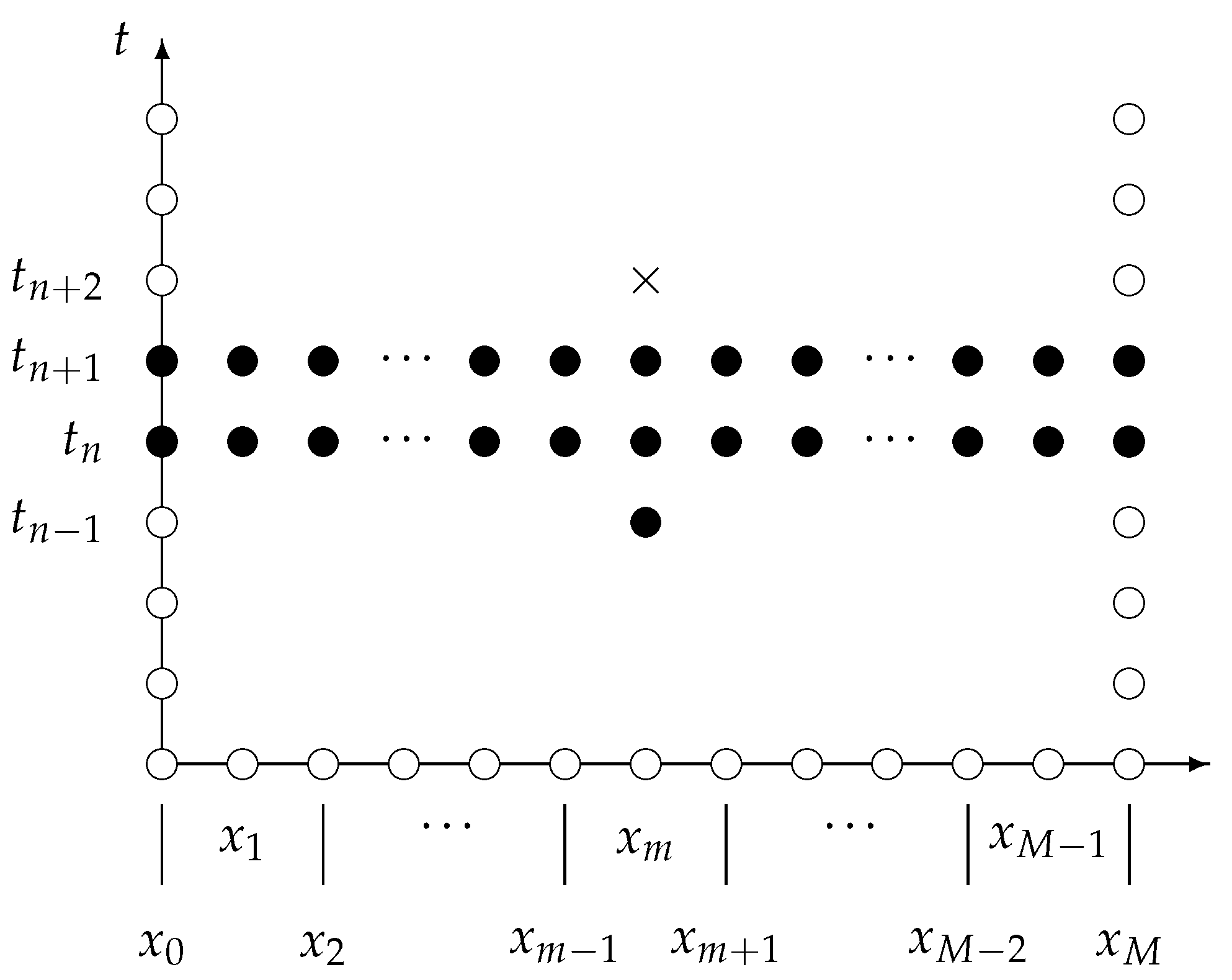
Here, the functions ${\varphi }_U,{\psi }_U,{\chi }_U:B\to \mathbb{R}$ are used to prescribe exactly the approximations at the times $t_0$, $t_1$ and $t_2$, respectively. The forward-difference stencil of the numerical model in Equation (30) is shown in Figure 1. Obviously, the finite-difference scheme is an explicit four-step technique, whence the existence and the uniqueness of numerical solutions is guaranteed for any set of initial data.

It is important to mention that the approximations at the times $t_1$ and $t_2$ can be computed in alternative forms. For example, one may try to approximate the first-order partial derivative with respect to time at the time $t=0$ using suitable finite-difference approximations. However, such approach could result in a loss of the quadratic consistency of the numerical model. Of course, this is a shortcoming of the present approach. Nevertheless, the scheme presents many other advantages, which are established thoroughly in the following, including its ability to preserve the energy in the undamped case, its quadratic consistency, its stability and its quadratic convergence. Needless to mention that the numerical model in Equation (30) can be easily implemented in any computer language.

Theorem 2 (Existence and uniqueness of solutions).

If $G,G_1,G_2,\dots ,G_p\in {\mathcal{C}}^1\left(\mathbb{R}\right)$, then the discrete problem in Equation (30) has a unique solution for each set of initial conditions.

Definition 10.

Let ${\left(U^n\right)}_{n\in {\overline{I}}_N}\subseteq {\mathcal{V}}_h$ be solution of the scheme in Equation (30). We define the discrete energy density as

$$H_m^n=\frac{1}{2}\left({\delta }_t{U}_m^{n+\frac{1}{2}}\right)\left({\delta }_t{U}_m^{n-\frac{1}{2}}\right)+G\left(U_m^n\right)+\sum _{j=1}^p{G}_j\left({\delta }_x^{({\alpha }_j/2)}{U}_m^n\right),\forall (m,n)\in J.$$

(31)

In turn, the total energy at the time $t_n$ is given by

$$E^n=h\sum _{m=0}^M{H}_m^n=\frac{1}{2}\langle {\delta }_t{U}^{n+\frac{1}{2}},{\delta }_t{U}^{n-\frac{1}{2}}\rangle +\langle G\left(U^n\right),1\rangle +\sum _{j=1}^p\langle G_j\left({\delta }_x^{({\alpha }_j/2)}{U}^n\right),1\rangle ,\forall n\in {\overline{I}}_{N-1}.$$

(32)

Lemma 3.

If ${\left(U^n\right)}_{n\in {\overline{I}}_N}\subseteq {\mathcal{V}}_h$, then the following identities are satisfied for each $n\in I_{N-2}$:

(a) 

$\langle {\widehat{\delta }}_t^{\left(2\right)}{U}^{n+\frac{1}{2}},{\delta }_t{U}^{n+\frac{1}{2}}\rangle =\frac{1}{2}{\delta }_t\langle {\delta }_t{U}^{n+\frac{1}{2}},{\delta }_t{U}^{n-\frac{1}{2}}\rangle$;

(b) 

$\langle {\delta }_t{U}^{n+\frac{1}{2}},{\delta }_t{U}^{n-\frac{1}{2}}\rangle ={\mu }_t\parallel {\delta }_t{U}^{n-\frac{1}{2}}{\parallel }_2^2-\frac{1}{2}{\tau }^2{\parallel {\delta }_t^{\left(2\right)}{U}^n\parallel }_2^2$;

(c) 

$\langle {\delta }_{U}G\left(U^{n+\frac{1}{2}}\right),{\delta }_t{U}^{n+\frac{1}{2}}\rangle ={\delta }_t\langle G\left(U^{n+\frac{1}{2}}\right),1\rangle$; and

(d) 

$\langle -{\delta }_x^{({\alpha }_j/2)}\left[{\delta }_{{\delta }_x^{({\alpha }_j/2)}U}{G}_j\left(U_m^{n+\frac{1}{2}}\right)\right],{\delta }_t{U}^{n+\frac{1}{2}}\rangle ={\delta }_t\langle G_j\left({\delta }_x^{({\alpha }_j/2)}{U}^{n+\frac{1}{2}}\right),1\rangle$.

Proof. 

To establish Identity (a), observe that

$$\langle {\widehat{\delta }}_t^{\left(2\right)}{U}^{n+\frac{1}{2}},{\delta }_t{U}^{n+\frac{1}{2}}\rangle =\frac{1}{2{\tau }^3}\langle U^{n+2}-U^{n+1}-U^n+U^{n-1},U^{n+1}-U^n\rangle =\frac{1}{2}{\delta }_t\langle {\delta }_t{U}^{n+\frac{1}{2}},{\delta }_t{U}^{n-\frac{1}{2}}\rangle .$$

(33)

Identities (b) and (c) are also straightforward, thus we only prove Identity (d). Notice that

$$\begin{array}{cc}\hfill & 〈-{\delta }_x^{({\alpha }_j/2)}\left[{\delta }_{{\delta }_x^{({\alpha }_j/2)}U}{G}_j\left(U_m^{n+\frac{1}{2}}\right)\right],{\delta }_t{U}^{n+\frac{1}{2}}〉=\frac{1}{\tau }〈{\delta }_{{\delta }_x^{({\alpha }_j/2)}U}{G}_j\left(U_m^{n+\frac{1}{2}}\right),{\delta }_x^{({\alpha }_j/2)}{U}^{n+1}-{\delta }_x^{({\alpha }_j/2)}{U}^n〉\hfill \\ \hfill & =\frac{1}{\tau }〈\frac{G_j\left({\delta }_x^{({\alpha }_j/2)}{U}^{n+1}\right)-G_j\left({\delta }_x^{({\alpha }_j/2)}{U}^n\right)}{{\delta }_x^{({\alpha }_j/2)}{U}^{n+1}-{\delta }_x^{({\alpha }_j/2)}{U}^n},{\delta }_x^{(\alpha /2)}{U}^{n+1}-{\delta }_x^{(\alpha /2)}{U}^n〉\hfill \\ \hfill & =\frac{1}{\tau }\left[\langle G_j\left({\delta }_x^{({\alpha }_j/2)}{U}^{n+1}\right),1\rangle -\langle G_j\left({\delta }_x^{({\alpha }_j/2)}{U}^n\right),1\rangle \right].\hfill \end{array}$$

(34)

Identity (d) readily follows now from these identities. □

Theorem 3 (Dissipation of discrete energy).

Let ${\left(U^n\right)}_{n\in {\overline{I}}_N}\subseteq {\mathcal{V}}_h$ be a solution of the finite-difference scheme in Equation (30). Then, ${\delta }_t{E}^{n+\frac{1}{2}}=-\gamma {\parallel {\delta }_t{U}^{n+\frac{1}{2}}\parallel }_2^2$, for each $n\in {\overline{I}}_{N-1}$. As a consequence, the discrete system in Equation (30) is conservative if $\gamma =0$. In general, the following identities holds:

$$\begin{array}{cc}\hfill E^n& =\frac{1}{2}{\mu }_t\parallel {\delta }_t{U}^{n-\frac{1}{2}}{\parallel }_2^2-\frac{{\tau }^2}{4}{\parallel {\delta }_t^{\left(2\right)}{U}^n\parallel }_2^2+\langle G\left(U^n\right),1\rangle +\sum _{j=1}^p\langle G_j\left({\delta }_x^{({\alpha }_j/2)}{U}^n\right),1\rangle \hfill \\ \hfill & =E^0-\gamma \tau \sum _{k=0}^{n-1}{\parallel {\delta }_t{U}^{k+\frac{1}{2}}\parallel }_2^2,\forall n\in I_{N-1}.\hfill \end{array}$$

(35)

Proof. 

We use the fact that ${\left(U^n\right)}_{n\in {\overline{I}}_N}$ satisfies the scheme in Equation (30) along with the identities of Lemma 3. Collecting terms and substituting the expression of the discrete total energy, we obtain

$$\begin{array}{cc}\hfill 0& =〈{\widehat{\delta }}_t^{\left(2\right)}{U}^{n+\frac{1}{2}}+\gamma {\delta }_t{U}^{n+\frac{1}{2}}+{\delta }_{U}G\left(U^{n+\frac{1}{2}}\right)-\sum _{j=1}^p{\delta }_x^{({\alpha }_j/2)}\left[{\delta }_{{\delta }_x^{({\alpha }_j/2)}U}{G}_j\left(U^{n+\frac{1}{2}}\right)\right],{\delta }_t{U}^{n+\frac{1}{2}}〉\hfill \\ \hfill & =\frac{1}{2}{\delta }_t\langle {\delta }_t{U}^{n+\frac{1}{2}},{\delta }_t{U}^{n-\frac{1}{2}}\rangle +\gamma {\parallel {\delta }_t{U}^{n+\frac{1}{2}}\parallel }_2^2+{\delta }_t\langle G\left(U^{n+\frac{1}{2}}\right),1\rangle +\sum _{j=1}^p{\delta }_t\langle G_j\left({\delta }_x^{({\alpha }_j/2)}{U}^{n+\frac{1}{2}}\right),1\rangle \hfill \\ \hfill & ={\delta }_t{E}^{n+\frac{1}{2}}+\gamma {\parallel {\delta }_t{U}^{n+\frac{1}{2}}\parallel }_2^2,\forall n\in {\overline{I}}_{N-1}.\hfill \end{array}$$

(36)

It readily follows that the discrete system is conservative if $\gamma =0$. The first identity of Equation (35) is reached now using Identity (b) of Lemma 3, while the second is obtained from Equation (36). □

4. Numerical Properties

The main numerical properties of the finite-difference scheme in Equation (30) are proved in the present section. More precisely, we establish rigorously the quadratic consistency of the scheme, the stability and its quadratic rate of convergence in both space and time. Various useful results are recalled or proved in the way, including a useful discrete Gronwall inequality and a technical proposition taken from the literature. Moreover, a novel auxiliary lemma is mathematically established, and we employ it to prove the stability and convergence of Equation (30).

In a first stage, we establish the consistency property of our scheme. To that end, we suppose that $u:\overline{\mathsf{\Omega }}\to \mathbb{R}$ is a function, and convey that $u_m^n=u(x_m,t_n)$, for each $(m,n)\in \overline{J}$. Let us introduce the differential and the difference operators $\mathcal{D}$ and D, which are defined by

$$\begin{array}{cc}\hfill \mathcal{D}u(x,t)& =\frac{{\partial }^{2}u(x,t)}{\partial t^2}+\gamma \frac{\partial u(x,t)}{\partial t}+\frac{dG\left(u\right(x,t\left)\right)}{dv}-\sum _{j=1}^p\frac{{\partial }^{{\alpha }_j/2}}{{\partial \left|x\right|}^{{\alpha }_j/2}}\frac{d{G}_j}{dv}\left(\frac{{\partial }^{{\alpha }_j/2}u(x,t)}{{\partial \left|x\right|}^{{\alpha }_j/2}}\right),\hfill \end{array}$$

(37)

$$\begin{array}{cc}\hfill D{u}_m^n& ={\widehat{\delta }}_t^{\left(2\right)}{u}_m^{n+\frac{1}{2}}+\gamma {\delta }_t{u}_m^{n+\frac{1}{2}}+{\delta }_{u}G\left(u_m^{n+\frac{1}{2}}\right)-\sum _{j=1}^p{\delta }_x^{({\alpha }_j/2)}\left[{\delta }_{{\delta }_x^{({\alpha }_j/2)}u}{G}_j\left(u_m^{n+\frac{1}{2}}\right)\right],\hfill \end{array}$$

(38)

for each $(x,t)\in \mathsf{\Omega }$ and $(m,n)\in J$. In our following results, we observe the discrete nomenclature $u^n=(u_0^n,u_1^n,\dots ,u_M^n)\in {\mathcal{V}}_h$, for each $n\in {\overline{I}}_M$.

Definition 11.

If $U={\left(U^n\right)}_{n\in {\overline{I}}_N}$ is a sequence in ${\mathcal{V}}_h$, then we define the real number

$${|\parallel U\parallel |}_{\infty }=max\{\parallel U^n{\parallel }_{\infty }:n\in {\overline{I}}_M\}.$$

(39)

Theorem 4

(Consistency). Let $u\in {\mathcal{C}}_{x,t}^{5,4}\left(\overline{\mathsf{\Omega }}\right)$ and suppose that $G\in {\mathcal{C}}^2\left(\mathbb{R}\right)$ and $G_1,G_2,\dots ,G_p\in {\mathcal{C}}^5\left(\mathbb{R}\right)$. Then, there exist constants $C,C^{\prime }\in {\mathbb{R}}^{+}$, which are independent of h and τ, such that

$$|\parallel \mathcal{L}u-{Lu\parallel |}_{\infty }\le C({\tau }^2+h^2)\mathit{and}|\parallel \mathcal{H}u-{Hu\parallel |}_{\infty }\le C^{\prime }(\tau +h^2).$$

(40)

Proof. 

Using Taylor’s theorem, it is easy to check that there exist constants $C_1,C_2,C_3,C_4^{\left(j\right)}\in {\mathbb{R}}^{+}$, which are independent of h and $\tau$, such that the following hold for each $j\in I_p$:

$$\begin{array}{cc}\hfill \left|\frac{{\partial }^{2}u(x_m,t_{n+\frac{1}{2}})}{\partial t^2}-{\widehat{\delta }}_t^{\left(2\right)}{u}_m^{n+\frac{1}{2}}\right|& \le C_1{\tau }^2,\forall (m,n)\in J,\hfill \end{array}$$

(41)

$$\begin{array}{cc}\hfill \left|\frac{\partial u(x_m,t_{n+\frac{1}{2}})}{\partial t}-{\delta }_t{u}_m^{n+\frac{1}{2}}\right|& \le C_2{\tau }^2,\forall (m,n)\in J,\hfill \end{array}$$

(42)

$$\begin{array}{cc}\hfill \left|\frac{dG\left(u(x_m,t_{n+\frac{1}{2}})\right)}{dv}-{\delta }_{u}G\left(u_m^{n+\frac{1}{2}}\right)\right|& \le C_3{\tau }^2,\forall (m,n)\in J,\hfill \end{array}$$

(43)

$$\begin{array}{cc}\hfill \left|\frac{{\partial }^{{\alpha }_j/2}}{{\partial \left|x\right|}^{{\alpha }_j/2}}\frac{d{G}_j}{dv}\left(\frac{{\partial }^{{\alpha }_j/2}u(x_m,t_{n+\frac{1}{2}})}{{\partial \left|x\right|}^{{\alpha }_j/2}}\right)-{\delta }_x^{({\alpha }_j/2)}\left[{\delta }_{{\delta }_x^{({\alpha }_j/2)}u}{G}_j\left(u_m^{n+\frac{1}{2}}\right)\right]\right|& \le C_4^{\left(j\right)}({\tau }^2+h^2),\forall (m,n)\in J.\hfill \end{array}$$

(44)

Let $C_4=max\{C_4^{\left(j\right)}:j\in I_p\}$. The first inequality of the conclusion follows then from the triangle inequality, letting $C=max\{C_1,\gamma C_2,C_3,C_4\}$. The second inequality is proved analogously. □

We turn our attention now to the properties of stability and convergence of the finite-difference scheme in Equation (30). To that end, the following well-known inequalities are needed in the sequel. We use them in the sequel without mentioning them explicitly:

(a)

If $U,V\in {\mathcal{V}}_h$, then $2\left|\langle U,V\rangle \right|\le {\parallel U\parallel }_2^2+{\parallel V\parallel }_2^2$.

(b)

If $n\in \mathbb{N}$ and $U^1,U^2,\dots ,U^n\in {\mathcal{V}}_h$, then

$$\parallel U^1+U^2+\dots +U^n{\parallel }_2^2\le n(\parallel U^1{\parallel }_2^2+\parallel U^2{\parallel }_2^2+\dots +\parallel U^n{\parallel }_2^2).$$

(45)

(c)

If ${\left(U^n\right)}_{n=0}^N\subseteq {\mathcal{V}}_h$ and $n\in I_N$, then

$$\parallel U^n{\parallel }_2^2\le 2\parallel U^0{\parallel }_2^2+2T\tau \sum _{k=0}^{n-1}{\parallel {\delta }_t{U}^k\parallel }_2^2,\forall n\in I_N.$$

(46)

The following auxiliary lemma has been taken from the literature. In the following, we let ${\mathsf{\Phi }}_U=({\varphi }_U,{\psi }_U,{\chi }_U)$, where ${\varphi }_U,{\psi }_U,{\chi }_U:B\to \mathbb{R}$ are functions and $U=V,W$.

Lemma 4

(Macías-Díaz [36]). Let $G\in {\mathcal{C}}^2\left(\mathbb{R}\right)$, and assume that ${\left(R^{n+\frac{1}{2}}\right)}_{n=0}^{N-1}$ is a sequence in ${\mathcal{V}}_h$. Moreover, suppose that ${\left(V^n\right)}_{n=0}^N$ and ${\left(W^n\right)}_{n=0}^N$ are two solutions of Equation (30) corresponding to ${\mathsf{\Phi }}_V$ and ${\mathsf{\Phi }}_W$, respectively. Let ${\epsilon }^n=V^n-W^n$ for each $n\in {\overline{I}}_N$, and define

$${\mathsf{\Lambda }}_{V,W}{G}^{n+\frac{1}{2}}={\delta }_{V}G\left(V^{n+\frac{1}{2}}\right)-{\delta }_{W}G\left(W^{n+\frac{1}{2}}\right),\forall n\in {\overline{I}}_{N-1}.$$

(47)

Then, there exists a constant $C^{\prime }\in {\mathbb{R}}^{+}\cup \left\{0\right\}$ which depends only on G, such that, for each $k\in I_{N-1}$,

$$\begin{array}{cc}\hfill 4\tau \sum _{n=1}^k\left|\langle R^{n+\frac{1}{2}}-{\mathsf{\Lambda }}_{V,W}{G}^{n+\frac{1}{2}},{\delta }_t{\epsilon }^{n+\frac{1}{2}}\rangle \right|& \le 4\tau \sum _{n=0}^k\parallel R^{n+\frac{1}{2}}{\parallel }_2^2+C^{\prime }\parallel {\epsilon }^0{\parallel }_2^2+C^{\prime }\tau \sum _{n=0}^k{\parallel {\delta }_t{\epsilon }^{n+\frac{1}{2}}\parallel }_2^2,\hfill \end{array}$$

(48)

$$\begin{array}{cc}\hfill 4k{\tau }^2\sum _{n=1}^k{\parallel {\mathsf{\Lambda }}_{V,W}{G}^{n+\frac{1}{2}}\parallel }_2^2& \le C^{\prime }{T}^2\parallel {\epsilon }^0{\parallel }_2^2+C^{\prime }{T}^3\tau \sum _{n=0}^k{\parallel {\delta }_t{\epsilon }^{n+\frac{1}{2}}\parallel }_2^2.\hfill \end{array}$$

(49)

Lemma 5.

Suppose that $G_j\in {\mathcal{C}}^2\left(\mathbb{R}\right)$ for each $j\in I_p$, and suppose that ${\left(V^n\right)}_{n=0}^N$ and ${\left(W^n\right)}_{n=0}^N$ are solutions of Equation (30) corresponding to ${\mathsf{\Phi }}_V$ and ${\mathsf{\Phi }}_W$, respectively. Let ${\epsilon }^n=V^n-W^n$ for each $n\in {\overline{I}}_N$, and define

$${\mathsf{\Theta }}_{V,W}{G}_j^{n+\frac{1}{2}}={\delta }_x^{({\alpha }_j/2)}\left[{\delta }_{{\delta }_x^{({\alpha }_j/2)}V}{G}_j\left(V^{n+\frac{1}{2}}\right)\right]-{\delta }_x^{({\alpha }_j/2)}\left[{\delta }_{{\delta }_x^{({\alpha }_j/2)}W}{G}_j\left(W^{n+\frac{1}{2}}\right)\right],\forall n\in {\overline{I}}_{N-1}.$$

(50)

Then, there exists a constant $C^{″}\in {\mathbb{R}}^{+}\cup \left\{0\right\}$ that depends only on G, such that, for each $k\in I_{N-1}$,

$$\begin{array}{cc}\hfill 4\tau \sum _{n=1}^k\sum _{j=1}^p\left|\langle {\mathsf{\Theta }}_{V,W}{G}_j^{n+\frac{1}{2}},{\delta }_t{\epsilon }^{n+\frac{1}{2}}\rangle \right|& \le C^{″}\parallel {\epsilon }^0{\parallel }_2^2+C^{″}\tau \sum _{n=0}^k{\parallel {\delta }_t{\epsilon }^{n+\frac{1}{2}}\parallel }_2^2,\hfill \end{array}$$

(51)

$$\begin{array}{cc}\hfill 4pk{\tau }^2\sum _{n=1}^k\sum _{j=1}^p{\parallel {\mathsf{\Theta }}_{V,W}{G}_j^{n+\frac{1}{2}}\parallel }_2^2& \le C^{″}{T}^2\parallel {\epsilon }^0{\parallel }_2^2+C^{″}{T}^3\tau \sum _{n=0}^k{\parallel {\delta }_t{\epsilon }^{n+\frac{1}{2}}\parallel }_2^2.\hfill \end{array}$$

(52)

Proof. 

Let $j\in I_p$. In the following chain of inequalities, we use firstly the square-root properties of fractional centered differences. Then, we employ Lemma 4 to show that there exists a constant $C_j^{\prime }\in {\mathbb{R}}^{+}\cup \left\{0\right\}$ that only depends on $G_j$, such that, for each $k\in I_{N-1}$,

$$\begin{array}{cc}\hfill & 4\tau \sum _{n=1}^k\left|\langle {\mathsf{\Theta }}_{V,W}{G}_j^{n+\frac{1}{2}},{\delta }_t{\epsilon }^{n+\frac{1}{2}}\rangle \right|=4\tau \sum _{n=1}^k\left|〈{\mathsf{\Lambda }}_{{\delta }_x^{({\alpha }_j/2)}V,{\delta }_x^{({\alpha }_j/2)}W}{G}_j^{n+\frac{1}{2}},{\delta }_t{\delta }_x^{({\alpha }_j/2)}{\epsilon }^{n+\frac{1}{2}}〉\right|\hfill \\ \hfill & \le C_j^{\prime }\parallel {\delta }_x^{({\alpha }_j/2)}{\epsilon }^0{\parallel }_2^2+C_j^{\prime }\tau \sum _{n=0}^k\parallel {\delta }_t{\delta }_x^{({\alpha }_j/2)}{\epsilon }^{n+\frac{1}{2}}{\parallel }_2^2\le C_j^{″}\parallel {\epsilon }^0{\parallel }_2^2+C_j^{″}\tau \sum _{n=0}^k{\parallel {\delta }_t{\epsilon }^{n+\frac{1}{2}}\parallel }_2^2.\hfill \end{array}$$

(53)

Here, $C_j^{″}=C_j^{\prime }{g}_h^{\left(\alpha \right)}$ in view of Lemma 2. It is clear that $C^{″}=C_1^{″}+C_2^{″}+\dots +C_p^{″}$. The second inequality of this result can be established in similar fashion from the second inequality of Lemma 4. □

The following discrete version of Gronwall’s inequality is of utmost importance.

Lemma 6

(Pen-Yu [54]). Let ${\left({\omega }^n\right)}_{n=0}^N$ and ${\left({\rho }^n\right)}_{n=0}^N$ be finite sequences of nonnegative mesh functions, and suppose that there exists $C\ge 0$ such that

$${\omega }^k\le {\rho }^k+C\tau \sum _{n=0}^{k-1}{\omega }^k,\forall k\in I_{N-1}.$$

(54)

Then, ${\omega }^n\le {\rho }^n{e}^{Cn\tau }$ for each $n\in {\overline{I}}_N$.

Theorem 5 (Stability).

Let $G,G_1,G_2,\dots ,G_p\in {\mathcal{C}}^2\left(\mathbb{R}\right)$. Suppose that ${\mathsf{\Phi }}_V$ and ${\mathsf{\Phi }}_W$ are two sets of initial conditions for Equation (30), and that ${\left(V^n\right)}_{n\in {\overline{I}}_N}$ and ${\left(W^n\right)}_{n\in {\overline{I}}_N}$ are the respective solutions. Let ${\epsilon }^n=V^n-W^n$ for each $n\in {\overline{I}}_N$, and define the nonnegative constants

$$\begin{array}{cc}\hfill {\omega }^k& =\parallel {\delta }_t{\epsilon }^{k+\frac{1}{2}}{\parallel }_2^2,\forall k\in I_{N-1},\hfill \end{array}$$

(55)

$$\begin{array}{cc}\hfill \rho & =C_1(1+T^2)\parallel {\epsilon }^0{\parallel }_2^2+2{\mu }_t\parallel {\delta }_t{\epsilon }^{\frac{1}{2}}{\parallel }_2^2+4T^2{\parallel {\delta }_t^{\left(2\right)}{\epsilon }^1\parallel }_2^2.\hfill \end{array}$$

(56)

Then, there is a constant $C\in {\mathbb{R}}^{+}\cup \left\{0\right\}$ independent of τ, such that ${\omega }^k\le \rho e^{CT}$, for each $k\in I_{N-1}$.

Proof. 

Notice that the sequences $V={\left(V^n\right)}_{n\in {\overline{I}}_N}$ and $W={\left(W^n\right)}_{n\in {\overline{I}}_N}$ satisfy the problem in Equation (30) with $U=V$ and $U=W$, respectively. Subtracting those problems, we obtain the discrete system

$$\begin{array}{c}{\displaystyle {\widehat{\delta }}_t^{\left(2\right)}{\epsilon }^{n+\frac{1}{2}}+\gamma {\delta }_t{\epsilon }^{n+\frac{1}{2}}+{\mathsf{\Lambda }}_{V,W}{G}^{n+\frac{1}{2}}-\sum _{j=1}^p{\mathsf{\Theta }}_{V,W}{G}_j^{n+\frac{1}{2}}=0,\forall (m,n)\in J,}\\ \mathrm{such}\mathrm{that}\left\{\begin{array}{cc}{\epsilon }_m^0={\varphi }_V\left(x_m\right)-{\varphi }_W\left(x_m\right),\hfill & \forall m\in I_{M-1},\hfill \\ {\epsilon }_m^1={\psi }_V\left(x_m\right)-{\psi }_W\left(x_m\right),\hfill & \forall m\in I_{M-1},\hfill \\ {\epsilon }_m^2={\chi }_V\left(x_m\right)-{\chi }_W\left(x_m\right),\hfill & \forall m\in I_{M-1},\hfill \\ {\epsilon }_0^n={\epsilon }_M^n=0,\hfill & \forall n\in {\overline{I}}_N.\hfill \end{array}\right.\end{array}$$

(57)

Let $k\in I_{N-2}$, and take the inner product of ${\delta }_t{\epsilon }^{n+\frac{1}{2}}$ with the vector difference equation of Equation (57) corresponding to the time $t_{n+\frac{1}{2}}$. To that end, we apply Identities (a) and (b) of Lemma 3 and rearrange terms. As a consequence, we obtain the expression

$$\frac{1}{2}{\delta }_t{\mu }_t\parallel {\delta }_t{\epsilon }^{n-\frac{1}{2}}{\parallel }_2^2=\frac{{\tau }^2}{4}{\delta }_t\parallel {\delta }_t^{\left(2\right)}{\epsilon }^n{\parallel }_2^2-〈{\mathsf{\Lambda }}_{V,W}{G}^{n+\frac{1}{2}}-\sum _{j=1}^p{\mathsf{\Theta }}_{V,W}{G}_j^{n+\frac{1}{2}},{\delta }_t{\epsilon }^{n+\frac{1}{2}}〉-\gamma {\parallel {\delta }_t{\epsilon }^{n+\frac{1}{2}}\parallel }_2^2.$$

(58)

Take now the sum on both sides of this equation over all indexes $n\in I_k$. Use the formula for telescoping sums to simplify algebraically, multiply then by $4\tau$ and add the term $2{\mu }_t{\parallel {\delta }_t{\epsilon }^{\frac{1}{2}}\parallel }_2^2$ on both sides of the identity. Use then Lemmas 4 and 5 to obtain

$$\begin{array}{cc}\hfill \parallel {\delta }_t{\epsilon }^{k+\frac{3}{2}}{\parallel }_2^2& \le 2{\mu }_t\parallel {\delta }_t{\epsilon }^{k+\frac{1}{2}}{\parallel }_2^2\le 2{\mu }_t\parallel {\delta }_t{\epsilon }^{\frac{1}{2}}{\parallel }_2^2+{\tau }^2{\parallel {\delta }_t^{\left(2\right)}{\epsilon }^{k+1}\parallel }_2^2+4\tau \sum _{n=1}^k\left|\langle {\mathsf{\Lambda }}_{V,W}{G}^{n+\frac{1}{2}},{\delta }_t{\epsilon }^{n+\frac{1}{2}}\rangle \right|\hfill \\ \hfill & +4\tau \sum _{n=1}^k\sum _{j=1}^p\left|\langle {\mathsf{\Theta }}_{V,W}{G}_j^{n+\frac{1}{2}},{\delta }_t{\epsilon }^{n+\frac{1}{2}}\rangle \right|\hfill \\ \hfill & \le 2{\mu }_t\parallel {\delta }_t{\epsilon }^{\frac{1}{2}}{\parallel }_2^2+{\tau }^2\parallel {\delta }_t^{\left(2\right)}{\epsilon }^{k+1}{\parallel }_2^2+C_1\parallel {\epsilon }^0{\parallel }_2^2+C_1\tau \sum _{n=0}^k{\parallel {\delta }_t{\epsilon }^{n+\frac{1}{2}}\parallel }_2^2,\forall k\in I_{N-2}.\hfill \end{array}$$

(59)

Here, we let $C_1=C^{\prime }+C^{″}$, where $C^{\prime }$ and $C^{″}$ are the constants in Lemmas 4 and 5, respectively. Now, multiply the nth difference equation of Equation (57) by ${(-1)}^{n-1}$ and take the sum for all $n\in I_k$. Using then telescoping sums, regrouping and inductions, it is easy to notice that

$${(-1)}^{k-1}{\delta }_t^{\left(2\right)}{\epsilon }^{k+1}+{\delta }_t^{\left(2\right)}{\epsilon }^1=\sum _{n=1}^k{(-1)}^n\left[\gamma {\delta }_t{\epsilon }^{n+\frac{1}{2}}+{\mathsf{\Lambda }}_{V,W}{G}^{n+\frac{1}{2}}-\sum _{j=1}^p{\mathsf{\Theta }}_{V,W}{G}_j^{n+\frac{1}{2}}\right],$$

(60)

for each $\forall k\in I_{N-2}$. Solve for ${\delta }_t^{\left(2\right)}{\epsilon }^{k+1}$ and calculate the Euclidean norm of this term. After rearranging terms, simplifying algebraically and using the second inequalities of Lemmas 4 and 5, we obtain

$$\begin{array}{cc}\hfill {\tau }^2{\parallel {\delta }_t^{\left(2\right)}{\epsilon }^{k+1}\parallel }_2^2& \le 4{\tau }^2\parallel {\delta }_t^{\left(2\right)}{\epsilon }^1{\parallel }_2^2+4{\gamma }^{2}k{\tau }^2\sum _{n=1}^k\parallel {\delta }_t{\epsilon }^{n+\frac{1}{2}}{\parallel }_2^2+4k{\tau }^2\sum _{n=1}^k{\parallel {\mathsf{\Lambda }}_{V,W}{G}^{n+\frac{1}{2}}\parallel }_2^2\hfill \\ \hfill & +4kp{\tau }^2\sum _{n=1}^k\sum _{j=1}^p{\parallel {\mathsf{\Theta }}_{V,W}{G}_j^{n+\frac{1}{2}}\parallel }_2^2\hfill \\ \hfill & \le 4{\tau }^2\parallel {\delta }_t^{\left(2\right)}{\epsilon }^1{\parallel }_2^2+4{\gamma }^{2}k{\tau }^2\sum _{n=1}^k\parallel {\delta }_t{\epsilon }^{n+\frac{1}{2}}{\parallel }_2^2+C_1{T}^2\parallel {\epsilon }^0{\parallel }_2^2+C_1{T}^3\tau \sum _{n=0}^k{\parallel {\delta }_t{\epsilon }^{n+\frac{1}{2}}\parallel }_2^2,\hfill \end{array}$$

(61)

for each $k\in I_{N-2}$. Combining Equations (59) and (61), and using the notation of this theorem, it follows that

$${\omega }^{k+1}\le \rho +(C_1+C_1{T}^3+4{\gamma }^{2}T)\sum _{n=0}^k{\parallel {\delta }_t{\epsilon }^{n+\frac{1}{2}}\parallel }_2^2,\forall k\in I_{N-2}.$$

(62)

The conclusion follows now from Lemma 6, letting $C=C_1+C_1{T}^3+4{\gamma }^{2}T$. □

Theorem 6 (Convergence).

Let $u\in {\mathcal{C}}_{x,t}^{5,4}\left(\overline{\mathsf{\Omega }}\right)$ be the exact solution of problem in Equation (6), and suppose that $G\in \mathcal{C}\left(\mathbb{R}\right)$ and $G_1,G_2,\dots ,G_p\in {\mathcal{C}}^5\left(\mathbb{R}\right)$. If Equation (30) has exact initial conditions, then the solution of Equations (30) in the $L_2$-norm has order of convergence $\mathcal{O}({\tau }^2+h^2)$.

Proof. 

The proof of this result is similar to that of Theorem 5. For that reason, we only provide an abridged argument. Throughout, let ${ϵ}^n=u^n-U^n$ for each $n\in {\overline{I}}_N$. Notice that the sequence ${\left({ϵ}^n\right)}_{n\in {\overline{I}}_N}$ satisfies the discrete problem

$$\begin{array}{c}{\displaystyle {\widehat{\delta }}_t^{\left(2\right)}{ϵ}^{n+\frac{1}{2}}+\gamma {\delta }_t{ϵ}^{n+\frac{1}{2}}+{\mathsf{\Lambda }}_{u,U}{G}^{n+\frac{1}{2}}-\sum _{j=1}^p{\mathsf{\Theta }}_{u,U}{G}_j^{n+\frac{1}{2}}=R_m^{n+\frac{1}{2}},\forall (m,n)\in J,}\\ \mathrm{such}\mathrm{that}\left\{\begin{array}{cc}{ϵ}_m^0={ϵ}_m^1={ϵ}_m^2=0,\hfill & \forall m\in I_{M-1},\hfill \\ {ϵ}_0^n={ϵ}_M^n=0,\hfill & \forall n\in {\overline{I}}_N,\hfill \end{array}\right.\end{array}$$

(63)

where $R_m^{n+\frac{1}{2}}$ is the local truncation error at the point $(x_m,t_{n+\frac{1}{2}})$. In light of Theorem 4, it follows that there exists a constant $C_0$ which is independent of $\tau$, such that ${|\parallel R\parallel |}_{\infty }\le C_0({\tau }^2+h^2)$. Take the inner product of ${\delta }_t{ϵ}^{n+\frac{1}{2}}$ with the nth vector equation of Equation (63), and then sum overall $n\in I_k$, for some $k\in I_{N-2}$. Rearrange terms and use the first inequalities of Lemmas 4 and 5 to obtain that

$$\begin{array}{cc}\hfill \parallel {\delta }_t{ϵ}^{k+\frac{3}{2}}{\parallel }_2^2& \le 2{\mu }_t\parallel {\delta }_t{ϵ}^{\frac{1}{2}}{\parallel }_2^2+{\tau }^2{\parallel {\delta }_t^{\left(2\right)}{ϵ}^{k+1}\parallel }_2^2+4\tau \sum _{n=1}^k\left|\langle R^{n+\frac{1}{2}}-{\mathsf{\Lambda }}_{V,W}{G}^{n+\frac{1}{2}},{\delta }_t{ϵ}^{n+\frac{1}{2}}\rangle \right|\hfill \\ \hfill & +4\tau \sum _{n=1}^k\sum _{j=1}^p\left|\langle {\mathsf{\Theta }}_{V,W}{G}_j^{n+\frac{1}{2}},{\delta }_t{ϵ}^{n+\frac{1}{2}}\rangle \right|\hfill \\ \hfill & \le 2{\mu }_t\parallel {\delta }_t{ϵ}^{\frac{1}{2}}{\parallel }_2^2+{\tau }^2\parallel {\delta }_t^{\left(2\right)}{ϵ}^{k+1}{\parallel }_2^2+4\tau \sum _{n=0}^k\parallel R^{n+\frac{1}{2}}{\parallel }_2^2+C_1\parallel {ϵ}^0{\parallel }_2^2+C_1\tau \sum _{n=0}^k{\parallel {\delta }_t{ϵ}^{n+\frac{1}{2}}\parallel }_2^2,\hfill \end{array}$$

(64)

for each $k\in I_{N-2}$. As in the proof of Theorem 5, we agree that $C_1=C^{\prime }+C^{″}$, where $C^{\prime }$ and $C^{″}$ are the constants in Lemmas 4 and 5, respectively. On the other hand, departing from the difference equation of Equation (63), using mathematical induction and performing some algebraic simplifications lead to the following identity, valid for each $\forall k\in I_{N-2}$:

$${\delta }_t^{\left(2\right)}{ϵ}^{k+1}={(-1)}^k{\delta }_t^{\left(2\right)}{ϵ}^1-\sum _{n=1}^k{(-1)}^{n+k}\left[\gamma {\delta }_t{ϵ}^{n+\frac{1}{2}}+{\mathsf{\Lambda }}_{V,W}{G}^{n+\frac{1}{2}}-\sum _{j=1}^p{\mathsf{\Theta }}_{V,W}{G}_j^{n+\frac{1}{2}}+R^{n+\frac{1}{2}}\right].$$

(65)

As a consequence, we notice that

$$\begin{array}{cc}\hfill {\tau }^2{\parallel {\delta }_t^{\left(2\right)}{ϵ}^{k+1}\parallel }_2^2& \le 5{\tau }^2\parallel {\delta }_t^{\left(2\right)}{ϵ}^1{\parallel }_2^2+5{\gamma }^{2}k{\tau }^2\sum _{n=1}^k\parallel {\delta }_t{ϵ}^{n+\frac{1}{2}}{\parallel }_2^2+5k{\tau }^2\sum _{n=1}^k{\parallel {\mathsf{\Lambda }}_{V,W}{G}^{n+\frac{1}{2}}\parallel }_2^2\hfill \\ \hfill & +5kp{\tau }^2\sum _{n=1}^k\sum _{j=1}^p\parallel {\mathsf{\Theta }}_{V,W}{G}_j^{n+\frac{1}{2}}{\parallel }_2^2+5k{\tau }^2\sum _{n=1}^k{\parallel R^{n+\frac{1}{2}}\parallel }_2^2\hfill \\ \hfill & \le 5T^2\parallel {\delta }_t^{\left(2\right)}{ϵ}^1{\parallel }_2^2+5{\gamma }^{2}T\tau \sum _{n=1}^k\parallel {\delta }_t{ϵ}^{n+\frac{1}{2}}{\parallel }_2^2+C_1^{\prime }{T}^2{\parallel {ϵ}^0\parallel }_2^2\hfill \\ \hfill & +C_1^{\prime }{T}^3\tau \sum _{n=0}^k\parallel {\delta }_t{ϵ}^{n+\frac{1}{2}}{\parallel }_2^2+5T\tau \sum _{n=1}^k{\parallel R^{n+\frac{1}{2}}\parallel }_2^2,\forall k\in I_{N-2}.\hfill \end{array}$$

(66)

Here, $C_1^{\prime }=\frac{5}{4}{C}_1$. Substitute now Equation (66) into Equation (64) and simplify. It is easy to check then that

$${\omega }^{k+1}\le {\rho }^{k+1}+C_2\tau \sum _{n=0}^k{\omega }^k,\forall k\in I_{N-2},$$

(67)

where $C_2=C_1+C_1^{\prime }{T}^3+5{\gamma }^{2}T$, and

$$\begin{array}{cc}\hfill {\omega }^k& =\parallel {\delta }_t{ϵ}^{k+\frac{1}{2}}{\parallel }_2^2,\forall k\in I_{N-1},\hfill \end{array}$$

(68)

$$\begin{array}{cc}\hfill {\rho }^k& =(C_1+C_1^{\prime }{T}^2)\parallel {ϵ}^0{\parallel }_2^2+2{\mu }_t\parallel {\delta }_t{ϵ}^{\frac{1}{2}}{\parallel }_2^2+5T^2\parallel {\delta }_t^{\left(2\right)}{ϵ}^1{\parallel }_2^2+(4+5T)\tau \sum _{n=0}^k{\parallel R^{n+\frac{1}{2}}\parallel }_2^2.\hfill \end{array}$$

(69)

Lemma 6 shows now that ${\omega }^k\le C_3{\rho }^k$ for all $k\in I_{N-1}$, where $C_3=e^{C_{2}T}$. However, recall that the initial conditions of Equation (63) are zero. In particular, this means that the first three terms on the right-hand side of Equation (68) are equal to zero, for all $k\in I_{N-2}$. This and the consistency property of the finite-difference scheme in Equation (30) imply that, for each $k\in I_{N-1}$,

$$\parallel {\delta }_t{ϵ}^{k+\frac{1}{2}}{\parallel }_2^2={\omega }^k\le C_3{\rho }^k=2C_3(1+8T)\tau \sum _{n=0}^{k-1}{\parallel R^{n+\frac{1}{2}}\parallel }_2^2\le C_4^2{({\tau }^2+h^2)}^2.$$

(70)

Here, $C_4^2=2C_0^2{C}_{3}T(4+5T)$. As a consequence, note that

$$\frac{1}{\tau }(\parallel {ϵ}^{k+1}{\parallel }_2-\parallel {ϵ}^k{\parallel }_2)\le \parallel {\delta }_t{ϵ}^{k+\frac{1}{2}}{\parallel }_2\le C_4({\tau }^2+h^2),\forall k\in I_{N-1}.$$

(71)

Telescoping sums and the fact that ${ϵ}^0=0$, yield the inequality

$$\parallel {ϵ}^n{\parallel }_2\le {\parallel {ϵ}^0\parallel }_2+C_4\tau n({\tau }^2+h^2)\le C({\tau }^2+h^2),\forall n\in I_N,$$

(72)

which is what we want to prove. Here, we just need to clarify that $C=C_{4}T$. □

5. Computer Simulations

The purpose of this section is to provide examples that illustrate the validity of Theorem 3. Various different scenarios are considered to that end.

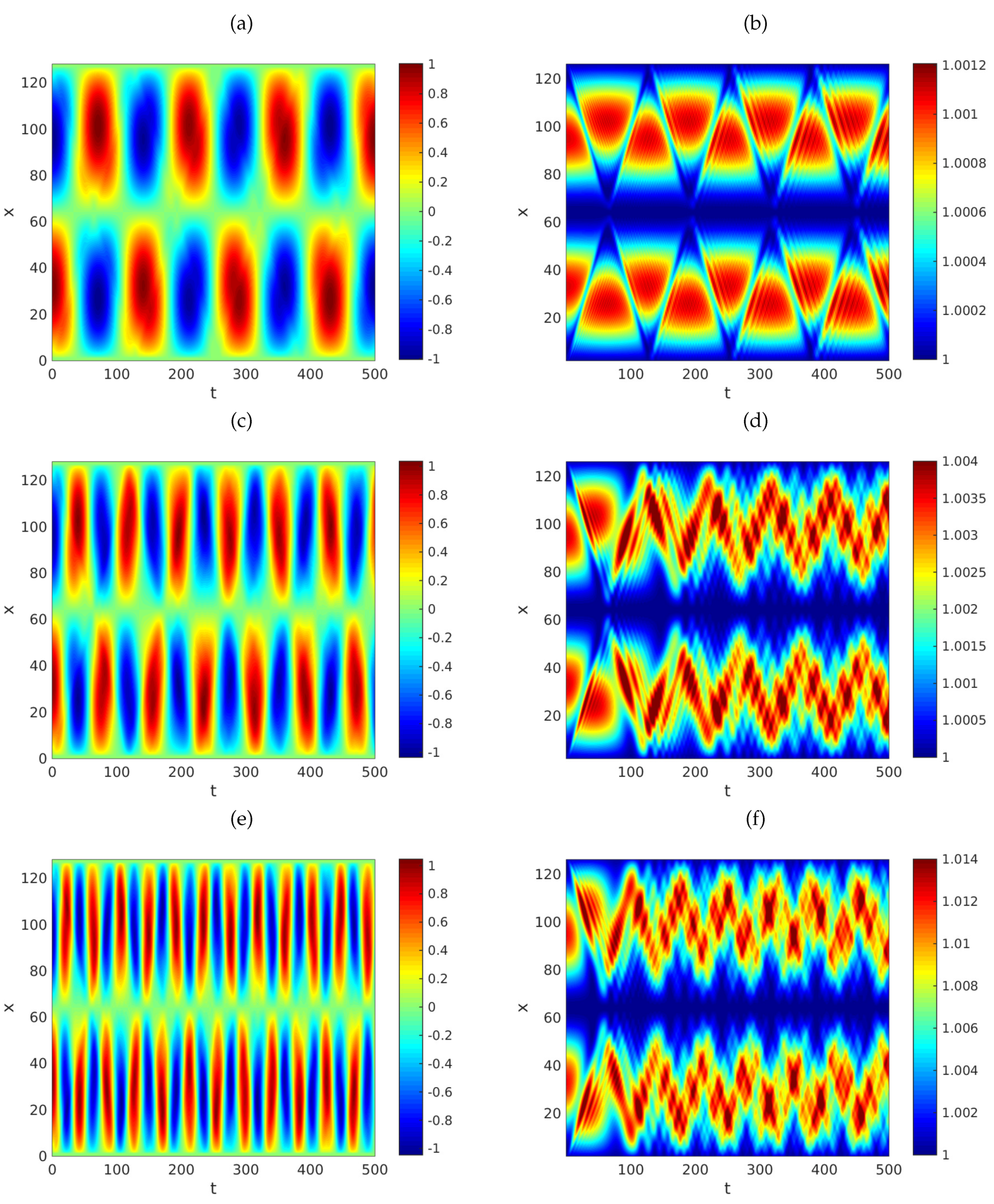
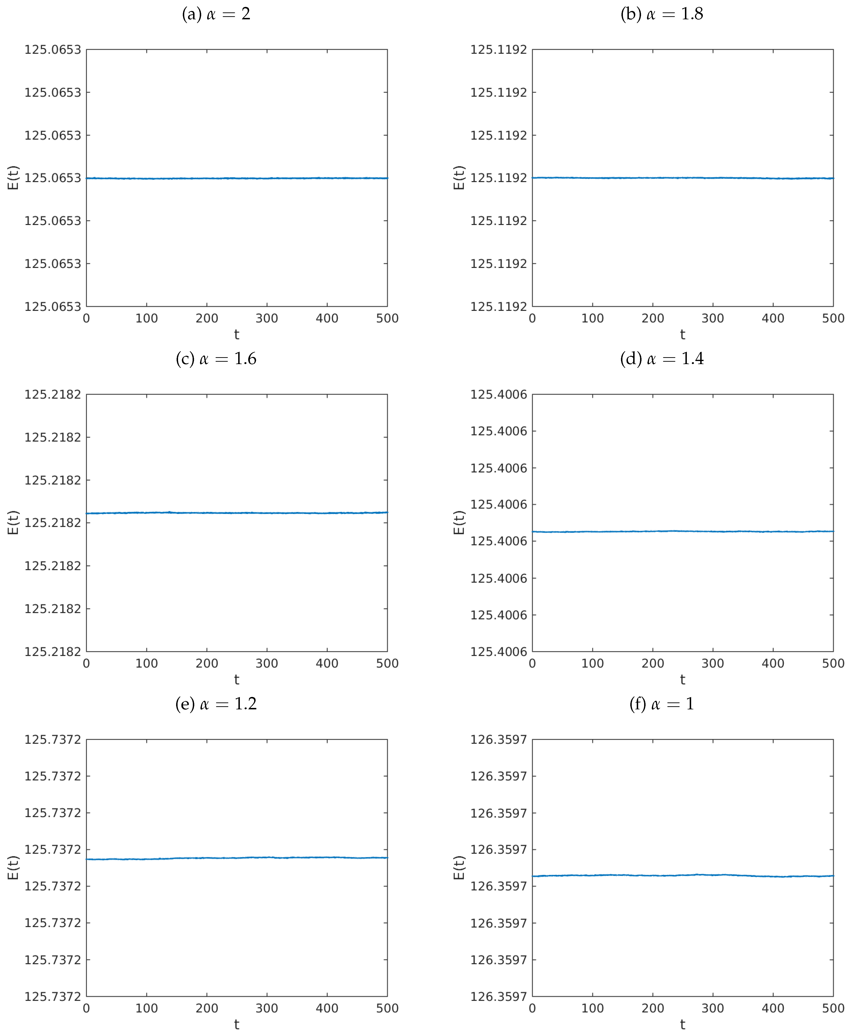
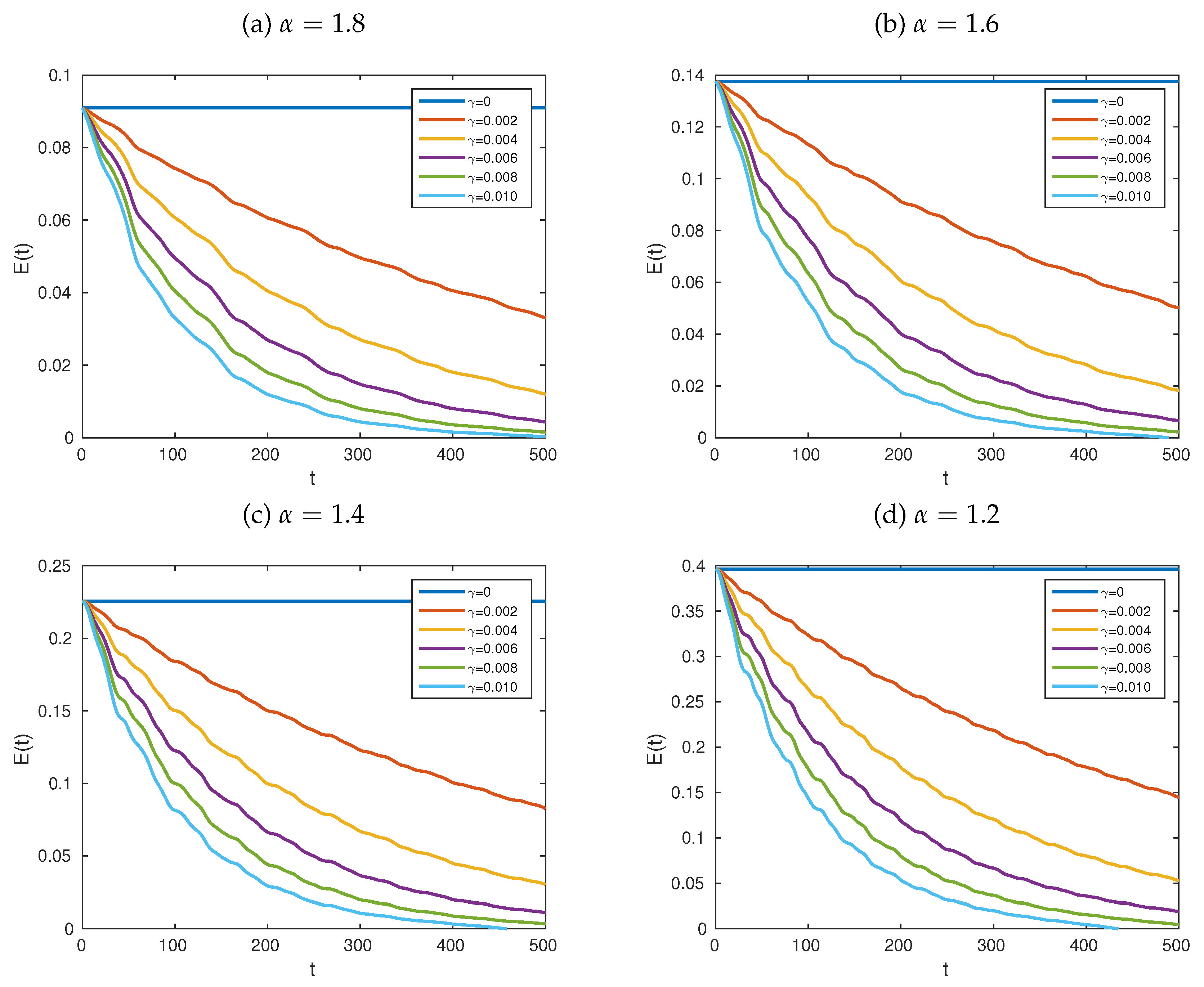
Example 2.

Let us consider the system in Equation (6) with $p=1$ and $\mathsf{\Omega }=(0,125)\times (0,200)$. We let $G\equiv 0$ and

$$G_1\left(v\right)=\sqrt{1+v^2},\forall v\in \mathbb{R}.$$

(73)

The resulting model describes a fractional version of a nonlinear vibration problem associated to an elastic string [55]. It is worth pointing out that this problem has interesting applications to the propagation of sounds and mechanical vibrations [56,57,58]. Fix the initial conditions as

$$\varphi \left(x\right)=\psi \left(x\right)=\chi \left(x\right)=sin(2\pi x/125),\forall x\in (0,125).$$

(74)

Computationally, we use the model in Equation (30) with $h=1$ and $\tau =0.025$, and agree that $\alpha ={\alpha }_1$. Under these circumstances, the left column of Figure 2 shows the approximate solutions of the problem for $\alpha =2$ (top row), $\alpha =1.6$ (middle row) and $\alpha =1.2$ (bottom row), using $\gamma =0$. Meanwhile, the right column shows the corresponding discrete energy densities. In turn, Figure 3 shows the dynamics of the total energy of the system for various values of α. These graphs confirm that the energy is conserved in the absence of damping. Figure 4 shows graphs of the total energy of the system for various values of α and γ. The results show that the total energy dissipates when damping is present. These remarks are in agreement with Theorem 3.

It is worth pointing out that our choice of the parameter $\tau$ in our previous example was obeying the need to provide a good approximation to the solution. Indeed, the value of $\tau$ is much smaller than that of h, but this choice was actually arbitrary. After all, the conditions to guarantee the stability and the convergence of the finite-difference scheme in Equation (30) are independent of the ratio of those parameters.

Example 3.

Let $\mathsf{\Omega }=(0,128)\times (0,500)$ and $ϵ=0.75$, and consider the system in Equation (6) with $p=1$, $G\equiv 0$ and

$$G_1\left(v\right)=\frac{1}{2}{v}^2+\frac{ϵ}{4}{v}^4,\forall v\in \mathbb{R}.$$

(75)

We approximate the exact solutions using Equation (30) with $h=1$ and $\tau =0.025$. As initial conditions, we set $\varphi \left(x\right)=v(x,0)$, $\psi \left(x\right)=v(x,\tau )$ and $\chi \left(x\right)=v(x,2\tau )$, for each $x\in (0,128)$. The function v is the algebraic sum of the well-known kink and anti-kink solutions of the Toda lattice [59], and it is given by the formula

$$v(x,t)=Aln\left\{\left(\frac{1+exp\left[2\right(\kappa (x-97)+tsinh\kappa \left)\right]}{1+exp\left[2\right(\kappa (x-96)+tsinh\kappa \left)\right]}\right)\left(\frac{1+exp\left[2\right(\kappa (x-32)+tsinh\kappa \left)\right]}{1+exp\left[2\right(\kappa (x-33)+tsinh\kappa \left)\right]}\right)\right\},$$

(76)

for each $(x,t)\in {\mathbb{R}}^2$. In our simulations, we let $A=5$, $\kappa =0.1$ and $\alpha ={\alpha }_1$. Figure 5 shows the approximate solutions of the corresponding problem in Equation (6) for $\alpha =2$ (top row), $\alpha =1.6$ (middle row) and $\alpha =1.2$ (bottom row), using $\gamma =0$. Note that the dynamics of the solutions and the energy density is similar to that reported in [50]. In turn, Figure 6 shows the dynamics of the total energy of the system, for various values of α and γ. The graphs confirm again that the energy is conserved in the absence of damping, and it is dissipated when damping is present.

The next example confirms the convergence rates derived in Theorem 6. For this purpose, we introduce the maximum-norm error between the exact solution of the continuous problem in Equation (6) at the time T, and the corresponding numerical approximation obtained through Equation (30), which is given by

$${ϵ}_{\tau ,h}=max\left\{\right|u_n^K-w_n^K|:n\in {\overline{I}}_N\}.$$

(77)

We also define the following standard rates:

$${\rho }_{\tau }={log}_2\left(\frac{{ϵ}_{2\tau ,h}}{{ϵ}_{\tau ,h}}\right),{\rho }_h={log}_2\left(\frac{{ϵ}_{\tau ,2h}}{{ϵ}_{\tau ,h}}\right).$$

(78)

Example 4.

Let us consider the same problem investigated in Example 3, with $\alpha ={\alpha }_1=1.5$. In particular, we employ the same space-time domain with the same model parameters, the same functions G and $G_1$, as well as the same initial data on $(0,128)$. The exact solution for this problem at the time $T=500$ is not known in exact form, but we estimate it using relatively small values of the computational parameters. To that effect, we set $h=4/2^8$ and $\tau =0.1/2^6$. Under these circumstances,

Table 1. Table of absolute errors in the maximum norm and temporal rates of convergence for various values of the parameters $\tau$ and h. The experiment corresponds to that described in Example 4.

	$\mathit{h}=1$		$\mathit{h}=0.5$		$\mathit{h}=0.25$
$\mathit{\tau }$	${\mathit{ϵ}}_{\mathit{t},\mathit{h}}$	${\mathit{\rho }}_{\mathit{\tau }}$	${\mathit{ϵ}}_{\mathit{t},\mathit{h}}$	${\mathit{\rho }}_{\mathit{\tau }}$	${\mathit{ϵ}}_{\mathit{t},\mathit{h}}$	${\mathit{\rho }}_{\mathit{\tau }}$
$0.1/2^0$	$2.6805\times {10}^{-2}$	−	$6.7596\times {10}^{-3}$	−	$1.6854\times {10}^{-3}$	−
$0.1/2^1$	$6.4470\times {10}^{-3}$	$2.0558$	$1.6881\times {10}^{-3}$	$2.0015$	$4.2704\times {10}^{-4}$	$1.9807$
$0.1/2^2$	$1.5595\times {10}^{-3}$	$2.0475$	$4.1406\times {10}^{-4}$	$2.0275$	$1.0711\times {10}^{-4}$	$1.9952$
$0.1/2^3$	$3.8014\times {10}^{-4}$	$2.0365$	$9.8730\times {10}^{-5}$	$2.0683$	$2.6528\times {10}^{-5}$	$2.0136$
$0.1/2^4$	$9.1697\times {10}^{-5}$	$2.0516$	$2.3789\times {10}^{-5}$	$2.0532$	$6.4825\times {10}^{-6}$	$2.0329$

shows the maximum-norm errors for various values of τ, keeping the parameter h constant. Additionally, the standard rates in time are provided in each case. The results show that the method has second order of convergence in time, in agreement with the conclusion of Theorem 6. In turn,

Table 2. Table of absolute errors in the maximum norm and spatial rates of convergence for various values of the parameters $\tau$ and h. The experiment corresponds to that described in Example 4.

	$\mathit{\tau }=5\times {10}^{-5}$		$\mathit{\tau }=2.5\times {10}^{-5}$		$\mathit{\tau }=1.25\times {10}^{-5}$
$\mathit{h}$	${\mathit{ϵ}}_{\mathit{t},\mathit{h}}$	${\mathit{\rho }}_{\mathit{h}}$	${\mathit{ϵ}}_{\mathit{t},\mathit{h}}$	${\mathit{\rho }}_{\mathit{h}}$	${\mathit{ϵ}}_{\mathit{t},\mathit{h}}$	${\mathit{\rho }}_{\mathit{h}}$
$4/2^0$	$7.1887\times {10}^{-3}$	−	$1.8178\times {10}^{-3}$	−	$4.5327\times {10}^{-4}$	−
$4/2^1$	$1.8250\times {10}^{-3}$	$1.9778$	$5.0045\times {10}^{-4}$	$1.8609$	$1.2482\times {10}^{-4}$	$1.8605$
$4/2^2$	$4.5941\times {10}^{-4}$	$1.9900$	$1.2724\times {10}^{-4}$	$1.9756$	$3.1762\times {10}^{-5}$	$1.9745$
$4/2^3$	$1.0807\times {10}^{-4}$	$2.0877$	$3.2302\times {10}^{-5}$	$1.9779$	$8.0961\times {10}^{-6}$	$1.9720$
$4/2^4$	$2.0730\times {10}^{-5}$	$2.3822$	$7.8347\times {10}^{-6}$	$2.0437$	$1.9029\times {10}^{-6}$	$2.0890$

shows the analysis of spatial convergence of the numerical model. The results confirm the quadratic rate of convergence of Equation (30), in agreement with Theorem 6 again.

The following examples provide hard numerical evidence on the quadratic order of convergence of the numerical model in Equation (30), as well as on its stability property.

Example 5.

The purpose of the present example is to provide more solid evidence on the temporal quadratic order of convergence of the scheme in Equation (30). To that end, let $p=1$ and $\mathsf{\Omega }=(0,1)\times (0,1000)$. Convey that $G\equiv 0$, and let $G_1$ be given as in Example 2. As initial data, we set

$$\varphi \left(x\right)=\psi \left(x\right)=\chi \left(x\right)=sin\left(2\pi x\right),\forall x\in (0,1).$$

(79)

For illustrative purposes, let us set ${\alpha }_1=1.6$ and $\gamma =0$. Under these conditions,

Table 3. Table of absolute errors in the maximum norm and temporal rates of convergence for various values of the parameters $\tau$ and h. The experiment corresponds to that described in Example 5.

	$\mathit{h}=1/2^4$		$\mathit{h}=1/2^5$		$\mathit{h}=1/2^6$
$\mathit{\tau }$	${\mathit{ϵ}}_{\mathit{t},\mathit{h}}$	${\mathit{\rho }}_{\mathit{\tau }}$	${\mathit{ϵ}}_{\mathit{t},\mathit{h}}$	${\mathit{\rho }}_{\mathit{\tau }}$	${\mathit{ϵ}}_{\mathit{t},\mathit{h}}$	${\mathit{\rho }}_{\mathit{\tau }}$
$1/2^3$	$2.7368\times {10}^{-4}$	−	$6.6597\times {10}^{-5}$	−	$1.6593\times {10}^{-5}$	−
$1/2^4$	$6.9872\times {10}^{-5}$	$1.9697$	$1.6889\times {10}^{-5}$	$1.9793$	$4.2431\times {10}^{-6}$	$1.9674$
$1/2^5$	$1.7664\times {10}^{-5}$	$1.9839$	$4.1418\times {10}^{-6}$	$2.0278$	$1.0723\times {10}^{-6}$	$1.9844$
$1/2^6$	$4.4770\times {10}^{-6}$	$1.9802$	$1.0341\times {10}^{-6}$	$2.0018$	$2.6944\times {10}^{-7}$	$1.9927$

provides a temporal analysis of convergence of the finite-difference scheme in Equation (30), considering various values of τ and h. The results of our simulations show that the numerical model exhibits a quadratic order of convergence, even in the case when the parameters h and τ are approximately equal. This result is in full agreement with Theorem 6.

Example 6.

Recall that one way to establish the stability of variational schemes is to show that the energy of the undamped system remains constant for long periods of time, using different values of the computational parameters. In the present example, we confirm this feature of our numerical model. To that end, we consider the same problem investigated in Example 3. That is, let $\alpha =1.5$, $\gamma =0$, $B=(0,128)$ and $ϵ=0.75$, and consider the model in Equation (6) with $p=1$, $G\equiv 0$ and $G_1$ given by Equation (75). Define $\varphi \left(x\right)=v(x,0)$, $\psi \left(x\right)=v(x,\tau )$ and $\chi \left(x\right)=v(x,2\tau )$, for each $x\in (0,128)$, where v is provided by Equation (76). Throughout, we set $T=1\times {10}^6$, and fix $h=1$. Under these circumstances, Figure 7 provides graphs of the dynamics of the total energy of the system versus t, for various values of τ. The range of the scale of the y-axis is the interval $[0.17103,0.17108]$. The result confirm that the total energy is approximately constant, as predicted by Theorem 3. These simulations provide support on the fact that the finite-difference scheme in Equation (30) is stable, even for values of τ which are larger than 1, and for all $\alpha \in (1,2]$. Obviously, this is in agreement with Theorem 5.

Before closing this section, it is worth pointing out that we carried out more numerical experiments. We do not include them in this paper to avoid redundancy, but they confirm the validity of the theoretical results obtained in this work.

6. Conclusions

In this work, we consider a general wave equation that encompasses various mathematical models from the physical sciences, including the sine-Gordon, the Klein–Gordon and the double sine-Gordon equations as well as continuous forms of the classical Fermi–Pasta–Ulam–Tsingou chains. The model under investigation includes the presence of constant damping, a nonlinear reaction term and general functions that depend on anomalous diffusion forms of the solution. In a first step, we show that the undamped form of the system has a variational structure. We propose functions for the local and total energy densities, and we show that the total energy is conserved or dissipated, depending on whether damping is absent or present, respectively. Motivated by these facts, we propose a finite-difference discretization of the continuous model, along with discrete forms of the local and total energy functionals. We show rigorously that the proposed discrete model is capable of reflecting the same energy properties of the continuous model. Moreover, we prove mathematically that the numerical model yields consistent approximations to the exact solutions of the continuous system, with quadratic order of consistency in both space and time.

To establish the properties of stability and convergence, we use various propositions. To start with, a discrete form of Gronwall’s inequality available in the literature is employed as the cornerstone of the proofs. Some other technical results are also recalled. However, the proofs of stability and convergence employ a novel technical proposition in order to bound appropriately the functions which depend on anomalous diffusion. As a result, we show that the proposed finite-difference scheme is stable, and that it converges to the exact solution of the continuous model with quadratic order of convergence in both space and time. To prove those results, suitable regularity conditions on the functions involved in the model are needed. For illustration purposes, we provide some computer simulations, which exhibited the capability of the scheme to conserve the energy when damping is absent and dissipate it when damping is present. The computer simulations were obtained using a computer implementation of our finite-difference scheme in Fortran 95. It is worth pointing out that the results of this work could be used in various potential applications, such as the investigation of nonlinear phenomena in generalized fractional systems [53,60], or even the transmission of signals in fractional forms of nonlinear media [61,62,63].

We would like to point out that the present work improves greatly various individual efforts by this author. As mentioned in the Introduction, some methodologies have been proposed already to solve fractional wave equations using fractional-order centered differences [35,36,37]. From the mathematical point of view, those previous efforts considered much simpler forms of the mathematical model in Equation (6). More precisely, in those articles, this author considered the initial-boundary-value problem

$$\begin{array}{c}{\displaystyle \frac{{\partial }^{2}u}{\partial t^2}(x,t)-\frac{{\partial }^{\alpha }u}{{\partial \left|x\right|}^{\alpha }}(x,t)+\gamma \frac{\partial u}{\partial t}(x,t)+G^{\prime }\left(u(x,t)\right)=0,\forall (x,t)\in \mathsf{\Omega },}\\ \mathrm{such}\mathrm{that}\left\{\begin{array}{cc}u(x,0)=\varphi \left(x\right),\hfill & \forall x\in (a,b),\hfill \\ {\displaystyle \frac{\partial u}{\partial t}(x,0)=\psi \left(x\right),}\hfill & \forall x\in (a,b),\hfill \\ u(a,t)=u(b,t)=0,\hfill & \forall t\in (0,T),\hfill \end{array}\right.\end{array}$$

(80)

Notice that the model in the present manuscript is both a dimensional and variational generalization of the problem in Equation (80). Indeed, it is easy to check that the mathematical problem in Equation (80) does not extend the Fermi–Pasta–Ulam–Tsingou problem to the fractional scenario. In that sense, the mathematical model in Equation (6) is a nontrivial extension of those investigated in [35,36,37].

On the other hand, from the numerical point of view, the present methodology presents the advantage of being relatively simple to implement. When compared to the approaches described in our previous papers, the present method is an explicit technique, which has the advantage of being numerically efficient under relatively light conditions. The obvious disadvantage here is the fact that the methodology is a four-step technique, and this fact implies the knowledge of the numerical solution at the first three time-steps. However, on the other hand, this disadvantage is compensated by the fact that the scheme is an energy-preserving method, and that the numerical efficiency analysis results in a relatively straightforward process. Moreover, the conditions under which the scheme is stable and convergent are little demanding in terms of the computational parameters. Additionally, the computer implementation of the scheme is also relatively straightforward, and it can be employed to investigate a wide range of problems in the physical sciences.

References

1. Arakawa, A.; Lamb, V.R. A potential enstrophy and energy conserving scheme for the shallow water equations. Mon. Weather Rev. 1981, 109, 18–36. [Google Scholar] [CrossRef]
2. Simmons, A.J.; Burridge, D.M. An energy and angular-momentum conserving vertical finite-difference scheme and hybrid vertical coordinates. Mon. Weather Rev. 1981, 109, 758–766. [Google Scholar] [CrossRef]
3. Pen-Yu, K.; Vázquez, L. Numerical solution of a nonlinear wave equation in polar coordinates. Appl. Math. Comput. 1984, 14, 313–329. [Google Scholar] [CrossRef]
4. Tang, Y.F.; Vázquez, L.; Zhang, F.; Pérez-García, V. Symplectic methods for the nonlinear Schrödinger equation. Comput. Math. Appl. 1996, 32, 73–83. [Google Scholar] [CrossRef]
5. Ben-Yu, G.; Pascual, P.J.; Rodriguez, M.J.; Vázquez, L. Numerical solution of the sine-Gordon equation. Appl. Math. Comput. 1986, 18, 1–14. [Google Scholar] [CrossRef]
6. Fei, Z.; Vázquez, L. Two energy conserving numerical schemes for the sine-Gordon equation. Appl. Math. Comput. 1991, 45, 17–30. [Google Scholar] [CrossRef]
7. Strauss, W.; Vazquez, L. Numerical solution of a nonlinear Klein-Gordon equation. J. Comput. Phys. 1978, 28, 271–278. [Google Scholar] [CrossRef]
8. Fei, Z.; Vázquez, L. Some conservative numerical schemes for an ordinary differential equation. Comput. Appl. Math. 1991, 10, 59–69. [Google Scholar]
9. Ibrahimbegovic, A.; Mamouri, S. Energy conserving/decaying implicit time-stepping scheme for nonlinear dynamics of three-dimensional beams undergoing finite rotations. Comput. Methods Appl. Mech. Eng. 2002, 191, 4241–4258. [Google Scholar] [CrossRef]
10. Romero, I.; Armero, F. An objective finite element approximation of the kinematics of geometrically exact rods and its use in the formulation of an energy–momentum conserving scheme in dynamics. Int. J. Numer. Methods Eng. 2002, 54, 1683–1716. [Google Scholar] [CrossRef]
11. Laursen, T.; Chawla, V. Design of energy conserving algorithms for frictionless dynamic contact problems. Int. J. Numer. Methods Eng. 1997, 40, 863–886. [Google Scholar] [CrossRef]
12. Furihata, D. A stable and conservative finite difference scheme for the Cahn-Hilliard equation. Numer. Math. 2001, 87, 675–699. [Google Scholar] [CrossRef]
13. Furihata, D.; Matsuo, T. A stable, convergent, conservative and linear finite difference scheme for the Cahn-Hilliard equation. Jpn. J. Ind. Appl. Math. 2003, 20, 65. [Google Scholar] [CrossRef]
14. Furihata, D. Finite-difference schemes for nonlinear wave equation that inherit energy conservation property. J. Comput. Appl. Math. 2001, 134, 37–57. [Google Scholar] [CrossRef]
15. Matsuo, T.; Furihata, D. Dissipative or conservative finite-difference schemes for complex-valued nonlinear partial differential equations. J. Comput. Phys. 2001, 171, 425–447. [Google Scholar] [CrossRef]
16. Furihata, D.; Matsuo, T. Discrete Variational Derivative Method: A Structure-Preserving Numerical Method for Partial Differential Equations; CRC Press: New York, NY, USA, 2010. [Google Scholar]
17. Ide, T.; Okada, M. Numerical simulation for a nonlinear partial differential equation with variable coefficients by means of the discrete variational derivative method. J. Comput. Appl. Math. 2006, 194, 425–459. [Google Scholar] [CrossRef]
18. Yaguchi, T.; Matsuo, T.; Sugihara, M. The discrete variational derivative method based on discrete differential forms. J. Comput. Phys. 2012, 231, 3963–3986. [Google Scholar] [CrossRef]
19. Furihata, D.; Sato, S.; Matsuo, T. A novel discrete variational derivative method using “average-difference methods”. JSIAM Lett. 2016, 8, 81–84. [Google Scholar] [CrossRef]
20. Suzuki, Y.; Ohnawa, M. Generic formalism and discrete variational derivative method for the two-dimensional vorticity equation. J. Comput. Appl. Math. 2016, 296, 690–708. [Google Scholar] [CrossRef]
21. Ishikawa, A.; Yaguchi, T. Application of the variational principle to deriving energy-preserving schemes for the Hamilton equation. JSIAM Lett. 2016, 8, 53–56. [Google Scholar] [CrossRef]
22. Kuramae, H.; Matsuo, T. An alternating discrete variational derivative method for coupled partial differential equations. JSIAM Lett. 2012, 4, 29–32. [Google Scholar] [CrossRef]
23. Ide, T. Some energy preserving finite element schemes based on the discrete variational derivative method. Appl. Math. Comput. 2006, 175, 277–296. [Google Scholar] [CrossRef]
24. Matsuo, T. Dissipative/conservative Galerkin method using discrete partial derivatives for nonlinear evolution equations. J. Comput. Appl. Math. 2008, 218, 506–521. [Google Scholar] [CrossRef]
25. Tomasiello, S. A note on three numerical procedures to solve Volterra integrodifferential equations in structural analysis. Comput. Math. Appl. 2011, 62, 3183–3193. [Google Scholar] [CrossRef]
26. Tomasiello, S. Some remarks on a new DQ-based method for solving a class of Volterra integro-differential equations. Appl. Math. Comput. 2012, 219, 399–407. [Google Scholar] [CrossRef]
27. Tarasov, V.E. Continuous limit of discrete systems with long-range interaction. J. Phys. A Math. Gen. 2006, 39, 14895. [Google Scholar] [CrossRef]
28. Koeller, R. Applications of fractional calculus to the theory of viscoelasticity. ASME Trans. J. Appl. Mech. 0021-8936 1984, 51, 299–307. [Google Scholar] [CrossRef]
29. Povstenko, Y. Theory of thermoelasticity based on the space-time-fractional heat conduction equation. Phys. Scr. 2009, 2009, 014017. [Google Scholar] [CrossRef]
30. Scalas, E.; Gorenflo, R.; Mainardi, F. Fractional calculus and continuous-time finance. Phys. A Stat. Mech. Appl. 2000, 284, 376–384. [Google Scholar] [CrossRef]
31. Glöckle, W.G.; Nonnenmacher, T.F. A fractional calculus approach to self-similar protein dynamics. Biophys. J. 1995, 68, 46–53. [Google Scholar] [CrossRef]
32. Namias, V. The fractional order Fourier transform and its application to quantum mechanics. IMA J. Appl. Math. 1980, 25, 241–265. [Google Scholar] [CrossRef]
33. Macías-Díaz, J.E. Sufficient conditions for the preservation of the boundedness in a numerical method for a physical model with transport memory and nonlinear damping. Comput. Phys. Commun. 2011, 182, 2471–2478. [Google Scholar] [CrossRef]
34. Macías-Díaz, J.E.; Villa-Morales, J. A deterministic model for the distribution of the stopping time in a stochastic equation and its numerical solution. J. Comput. Appl. Math. 2017, 318, 93–106. [Google Scholar] [CrossRef]
35. Macías-Díaz, J.E. A structure-preserving method for a class of nonlinear dissipative wave equations with Riesz space-fractional derivatives. J. Comput. Phys. 2017, 351, 40–58. [Google Scholar] [CrossRef]
36. Macías-Díaz, J.E. An explicit dissipation-preserving method for Riesz space-fractional nonlinear wave equations in multiple dimensions. Commun. Nonlinear Sci. Numer. Simul. 2018, 59, 67–87. [Google Scholar] [CrossRef]
37. Macías-Díaz, J.E. On the solution of a Riesz space-fractional nonlinear wave equation through an efficient and energy-invariant scheme. Int. J. Comput. Math. 2018, 96, 337–361. [Google Scholar] [CrossRef]
38. Alikhanov, A.A. A new difference scheme for the time fractional diffusion equation. J. Comput. Phys. 2015, 280, 424–438. [Google Scholar] [CrossRef] [Green Version]
39. Bhrawy, A.H.; Abdelkawy, M.A. A fully spectral collocation approximation for multi-dimensional fractional Schrödinger equations. J. Comput. Phys. 2015, 294, 462–483. [Google Scholar] [CrossRef]
40. El-Ajou, A.; Arqub, O.A.; Momani, S. Approximate analytical solution of the nonlinear fractional KdV–Burgers equation: A new iterative algorithm. J. Comput. Phys. 2015, 293, 81–95. [Google Scholar] [CrossRef]
41. Liu, F.; Zhuang, P.; Turner, I.; Anh, V.; Burrage, K. A semi-alternating direction method for a 2-D fractional FitzHugh–Nagumo monodomain model on an approximate irregular domain. J. Comput. Phys. 2015, 293, 252–263. [Google Scholar] [CrossRef] [Green Version]
42. Vázquez, L.; Trujillo, J.; Velasco, M.P. Fractional heat equation and the second law of thermodynamics. Fract. Calc. Appl. Anal. 2011, 14, 334–342. [Google Scholar] [CrossRef]
43. Veeresha, P.; Prakasha, D.G.; Baleanu, D. An efficient numerical technique for the nonlinear fractional Kolmogorov–Petrovskii–Piskunov equation. Mathematics 2019, 7, 265. [Google Scholar] [CrossRef] [Green Version]
44. Khan, H.; Shah, R.; Kumam, P.; Baleanu, D.; Arif, M. An efficient analytical technique, for the solution of fractional-order Telegraph equations. Mathematics 2019, 7, 426. [Google Scholar] [CrossRef] [Green Version]
45. Az-Zo’bi, E.A.; Al-Khaled, K.; Darweesh, A. Numeric-analytic solutions for nonlinear oscillators via the modified multi-stage decomposition method. Mathematics 2019, 7, 550. [Google Scholar] [CrossRef] [Green Version]
46. Fermi, E.; Pasta, P.; Ulam, S.; Tsingou, M. Studies of the Nonlinear Problems; Technical Report; Los Alamos Scientific Laboratory: Los Alamos, NM, USA, 1955. [Google Scholar]
47. Mickens, R.E. Dynamic consistency: A fundamental principle for constructing nonstandard finite difference schemes for differential equations. J. Differ. Equ. Appl. 2005, 11, 645–653. [Google Scholar] [CrossRef]
48. Laskin, N. Fractional Schrödinger equation. Phys. Rev. E 2002, 66, 056108. [Google Scholar] [CrossRef] [Green Version]
49. Friedman, A. Foundations of Modern Analysis; Courier Corporation: New York, NY, USA, 1970. [Google Scholar]
50. Macías-Díaz, J.E.; Medina-Ramírez, I.E. An implicit four-step computational method in the study on the effects of damping in a modified α-Fermi–Pasta–Ulam medium. Commun. Nonlinear Sci. Numer. Simul. 2009, 14, 3200–3212. [Google Scholar] [CrossRef]
51. Macías-Díaz, J.E. An explicit finite-difference method for the approximate solutions of a generic class of anharmonic dissipative nonlinear media. Numer. Methods Partial Differ. Equ. 2010, 26, 1351–1376. [Google Scholar] [CrossRef]
52. Wang, X.; Liu, F.; Chen, X. Novel second-order accurate implicit numerical methods for the Riesz space distributed-order advection-dispersion equations. Adv. Math. Phys. 2015, 2015, 590435. [Google Scholar] [CrossRef]
53. Macías-Díaz, J.E. Numerical simulation of the nonlinear dynamics of harmonically driven Riesz-fractional extensions of the Fermi–Pasta–Ulam chains. Commun. Nonlinear Sci. Numer. Simul. 2018, 55, 248–264. [Google Scholar] [CrossRef]
54. Pen-Yu, K. Numerical methods for incompressible viscous flow. Sci. Sin. 1977, 20, 287–304. [Google Scholar]
55. Carrier, G. On the non-linear vibration problem of the elastic string. Q. Appl. Math. 1945, 3, 157–165. [Google Scholar] [CrossRef] [Green Version]
56. Narasimha, R. Non-linear vibration of an elastic string. J. Sound Vib. 1968, 8, 134–146. [Google Scholar] [CrossRef]
57. Välimäki, V.; Pakarinen, J.; Erkut, C.; Karjalainen, M. Discrete-time modelling of musical instruments. Rep. Prog. Phys. 2005, 69, 1. [Google Scholar] [CrossRef] [Green Version]
58. Medina-Ramírez, I.; González-García, M.; Liu, J.L. Nanostructure characterization of polymer-stabilized gold nanoparticles and nanofilms derived from green synthesis. J. Mater. Sci. 2009, 44, 6325–6332. [Google Scholar] [CrossRef]
59. Toda, M. Waves in nonlinear lattice. Prog. Theor. Phys. Suppl. 1970, 45, 174–200. [Google Scholar] [CrossRef]
60. Macías-Díaz, J.E. Persistence of nonlinear hysteresis in fractional models of Josephson transmission lines. Commun. Nonlinear Sci. Numer. Simul. 2017, 53, 31–43. [Google Scholar] [CrossRef]
61. Macías-Díaz, J.E. Numerical study of the transmission of energy in discrete arrays of sine-Gordon equations in two space dimensions. Phys. Rev. E 2008, 77, 016602. [Google Scholar] [CrossRef]
62. Macías-Díaz, J.E.; Puri, A. On the propagation of binary signals in damped mechanical systems of oscillators. Phys. D Nonlinear Phenom. 2007, 228, 112–121. [Google Scholar] [CrossRef] [Green Version]
63. Macías-Díaz, J.E.; Puri, A. On the transmission of binary bits in discrete Josephson-junction arrays. Phys. Lett. A 2008, 372, 5004–5010. [Google Scholar] [CrossRef] [Green Version]
Figure 1. Forward-difference stencil for the approximation to the exact solution of the partial differential equation of Equation (6) at the time t n , using the finite-difference scheme in Equation (30). The black circles represent the known approximations at the times t n 1 , t n and t n + 1 , while the cross denotes the unknown approximation at the time t n + 2 .
Mathematics 07 01095 g001
Figure 2. Graphs of the approximate solution (a,c,e) and respective energy densities (b,d,f) of the system in Equation (6) versus t and x. The fractional partial differential equation considers γ = 0 and Ω = ( 0 , 125 ) × ( 0 , 500 ) . The initial data were defined by the functions ϕ ( x ) = ψ ( x ) = χ ( x ) = sin ( 2 π x / 125 ) , for each x ( 0 , 125 ) . Computationally, we fixed h = 1 and τ = 0.025 . We employed α = α 1 , with α = 2 (a,b), α = 1.6 (c,d) and α = 1.2 (e,f). The remaining parameters are p = 1 , G 0 , and G 1 is given by Equation (73).
Mathematics 07 01095 g002
Figure 3. Graphs of the dynamics of the total energy of the system in Equation (6) for various values of α = α 1 . The fractional partial differential equation considers γ = 0 and Ω = ( 0 , 125 ) × ( 0 , 500 ) . The initial data were defined by the functions ϕ ( x ) = ψ ( x ) = χ ( x ) = sin ( 2 π x / 125 ) , for each x ( 0 , 125 ) . Computationally, we fixed h = 1 and τ = 0.025 . The remaining parameters are p = 1 , G 0 , and G 1 is given by Equation (73).
Mathematics 07 01095 g003
Figure 4. Graphs of the dynamics of the total energy of the system in Equation (6) for various values of α = α 1 . The fractional partial differential equation considers Ω = ( 0 , 125 ) × ( 0 , 500 ) , and different values of γ . The initial data were defined by the functions ϕ ( x ) = ψ ( x ) = χ ( x ) = sin ( 2 π x / 125 ) , for each x ( 0 , 125 ) . Computationally, we fixed h = 1 and τ = 0.025 . The remaining parameters are p = 1 , G 0 , and G 1 is given by Equation (73).
Mathematics 07 01095 g004
Figure 5. Graphs of the approximate solution (a,c,e) and respective energy densities (b,d,f) of the system in Equation (6) versus t and x. The parameters employed are p = 1 , G 0 , and G 1 is given by Equation (75). We used ϵ = 0.75 , γ = 0 and Ω = ( 0 , 128 ) × ( 0 , 500 ) . The initial data were defined by the functions ϕ ( x ) = v ( x , 0 ) , ψ ( x ) = v ( x , τ ) and χ ( x ) = v ( x , 2 τ ) , for each x ( 0 , 32 ) . Here, v is the function defined by Equation (76). Computationally, we fixed h = 1 and τ = 0.025 . We employed α = α 1 with α = 2 (a,b), α = 1.6 (c,d) and α = 1.2 (e,f).
Mathematics 07 01095 g005
Figure 6. Graphs of the dynamics of the total energy of the system in Equation (6) for α = α 1 with (a) α = 1.8 , (b) α = 1.6 , (c) α = 1.4 and (d) α = 1.2 . The parameters employed are p = 1 , G 0 , and G 1 is given by Equation (75). We used ϵ = 0.75 and Ω = ( 0 , 128 ) × ( 0 , 500 ) . The initial data were defined by the functions ϕ ( x ) = v ( x , 0 ) , ψ ( x ) = v ( x , τ ) and χ ( x ) = v ( x , 2 τ ) , for each x ( 0 , 32 ) . Here, v is the function defined by Equation (76). Computationally, we fixed h = 1 and τ = 0.025 . In each case, we used the values of γ shown within the legend at the bottom of each graph.
Mathematics 07 01095 g006
Figure 7. Graphs of the total energy of the system in Equation (6) versus t. The parameters employed are p = 1 , G 0 , and G 1 is given by Equation (75). We used ϵ = 0.75 , α = 1.5 , γ = 0 , B = ( 0 , 128 ) and T = 1 × 10 6 . The initial data were defined by the functions ϕ ( x ) = v ( x , 0 ) , ψ ( x ) = v ( x , τ ) and χ ( x ) = v ( x , 2 τ ) , for each x ( 0 , 32 ) . Here, v is the function defined by Equation (76). Computationally, we fixed h = 1 , and we employed: (a) τ = 4 ; (b) τ = 2 ; (c) τ = 1 ; (d) τ = 0.5 ; (e) τ = 0.25 ; and (f) τ = 0.125 . The range of the scale of the y-axis is the interval [ 0.17103 , 0.17108 ] .
Mathematics 07 01095 g007aMathematics 07 01095 g007b