Continuum Modeling of Discrete Plant Communities: Why Does It Work and Why Is It Advantageous?

Abstract

Understanding ecosystem response to drier climates calls for modeling the dynamics of dryland plant populations, which are crucial determinants of ecosystem function, as they constitute the basal level of whole food webs. Two modeling approaches are widely used in population dynamics, individual (agent)-based models and continuum partial-differential-equation (PDE) models. The latter are advantageous in lending themselves to powerful methodologies of mathematical analysis, but the question of whether they are suitable to describe small discrete plant populations, as is often found in dryland ecosystems, has remained largely unaddressed. In this paper, we first draw attention to two aspects of plants that distinguish them from most other organisms—high phenotypic plasticity and dispersal of stress-tolerant seeds—and argue in favor of PDE modeling, where the state variables that describe population sizes are not discrete number densities, but rather continuous biomass densities. We then discuss a few examples that demonstrate the utility of PDE models in providing deep insights into landscape-scale behaviors, such as the onset of pattern forming instabilities, multiplicity of stable ecosystem states, regular and irregular, and the possible roles of front instabilities in reversing desertification. We briefly mention a few additional examples, and conclude by outlining the nature of the information we should and should not expect to gain from PDE model studies.

1. Introduction

Global warming and the concomitant increased frequency of intense droughts threaten the viability of plant populations and communities throughout the world [1,2,3]. As plants are primary producers that constitute the basal levels of whole food webs, that threat extends to ecosystem function as well. Understanding ecosystem response to drier climates, therefore, calls for unraveling mechanisms by which plant populations tolerate water stress. Such mechanisms operate at the organism level through various forms of phenotypic changes, but also at higher organization levels through self-organization in spatial patterns. These response forms are particularly relevant in dryland ecosystems, where both phenotypic changes and spatial self-organization are highly significant.

Empirical studies of plant-community dynamics are hampered by the long time-scales of plant growth and the yet longer time scales of self-organization in space. A powerful methodology that complements empirical studies and compensates for the time-scale limitation is the construction and study of dynamic mathematical models. These models can be divided into two major groups. The first group consists of individual-based models (IBM) (also called agent-based models), which are stochastic computational algorithms for interacting individual organisms. Each individual is described by a set of time-dependent attributes, often including its spatial location on a grid and various physiological and behavioral traits [4,5,6]. The second group of models consists of continuum partial differential equations (PDE) that do not address discrete individual organisms, but rather deterministic processes at small spatial scales. The population is then described by a variable that represents the population size, such as the population number density, and is considered to be continuous in time and space [7,8,9].

The advantage of PDE models over IBM is that they lend themselves to the powerful methods of dynamical-system and pattern-formation theories, and therefore can provide deeper insights into the mechanisms that drive ecosystem dynamics and ecosystem response to environmental variability [8,10,11]. However, the application of the PDE modeling approach to plant populations in drylands should first be justified, as these populations are typically small, especially in arid regions, where the vegetation is sparse. This inherent character of drylands questions the use of continuous variables to describe population sizes; variables, such as number densities, become highly discrete, and demographic noise and extinction may become important aspects of the dynamics [12,13].

In this paper, we first argue that the discrete nature of small plant populations may still be discarded in modeling their dynamics owing to the high phenotypic plasticity of plants. That calls for a different description of the population size; rather than describing it by a discrete number density, we describe it by a biomass variable, which remains continuous even at the level of a single plant. We further demonstrate with a few examples the advantage of continuum PDE modeling over discrete IBM and discuss the ecological significance of this advantage. The examples include the use of linear stability analysis to calculate thresholds for the emergence of periodic patterns, the use of numerical continuation to calculate bifurcation diagrams, and a study of a transverse instability of desertification fronts. We conclude the paper with a brief discussion of additional examples that demonstrate the utility of continuum PDE models in gaining mechanistic information and insights about large, landscape-scale behaviors.

2. Distinctive Aspects of Plant Populations

Population size is often described by the number density of the individuals that constitute the population. We describe here two distinctive properties of plants, not shared by most other organisms: high phenotypic plasticity and seed dispersal, that will be used in Section 3 to motivate a better way of describing plant population size, especially in drylands where the vegetation is often sparse.

2.1. Phenotypic Plasticity and Plant Adaptation to Variable Environments

Phenotypic plasticity is defined as the ability of an organism (or a given genotype) to give rise to distinct observable traits (phenotypes) when exposed to variable environmental conditions [14]. Two basic, distinct developmental approaches have been evolved in plants and animals reflecting different degrees of phenotypic plasticity. Animals have a relatively short period of embryonic phase prior to birth, whereby all major organs are formed and postnatal development is essentially restricted to expansion and growth of existing organs. By contrast, plants spend most of their life, from weeks and months to hundreds and often thousands of years, at the embryonic phase, in the sense that they can produce new organs (stems, leaves, flowers) throughout their life, depending on environmental conditions. The higher phenotypic plasticity of plants can be attributed to their sessile nature and their inability to migrate to less stressful conditions as mobile animals do.

A plant embryo has only a small fraction of the organs an adult body has, consisting of two apical meristems located at the tip of the shoot and the root, which are responsible for growth and expansion of the shoot and the root systems. Both meristems consist of pluripotent cells (cells capable of differentiation into multiple cell types that make up the plant body) that are functionally equivalent to animal stem cells [15]. The shoot apical meristem (SAM) gives rise to the production of the aerial part of the plant including leaves and axillary buds (from which new stems emerge) as well as flowers. The root apical meristem (RAM) allows the growth and development of the root system and its expansion below ground. Thus, while the SAM activity leads to the expansion of the photosynthetic activity, which is carbon fixation by light energy, the RAM activity enhances uptake and mobilization of water and minerals to the canopy.

The proportion between aboveground (shoot system) biomass and belowground (root system) biomass, the so-called root-to-shoot ratio, is dynamic and needs to be balanced to achieve optimal performance (and therefore survival) under variable environmental conditions. Commonly there is a positive correlation between shoot growth and root growth, and both are interconnected [16]. Accordingly, shoot growth provides ample energy for the expansion of the root system, which in turn increases water and nutrient uptake from a larger belowground domain to feed and enable the expansion of the shoot system, a mechanism that plays an important role in the development of vegetation patterns (see root-augmentation feedback in Section 3.1.2).

The capacity of plants to dynamically change the allocation of biomass to different organs is central to plant response to variable environments and crucial for plant survival. A well-known example of periodic change in above-ground (shoot) biomass is the shedding of leaves in temperate deciduous forests during the winter (when leaves are susceptible to cold and are not photosynthetically active) as a mechanism to tolerate low winter temperature, e.g., saving energy via remobilization and storage of leaf nutritional constituents in stems. Shedding of leaves may also occur during the dry season in tropical and subtropical deciduous forests as a mechanism to tolerate seasonal drought by reducing the loss of water through transpiration.

Plants thriving in variable desert environments show many additional mechanisms to cope with seasonal climate variations that involve changes in above-ground biomass. A good example of such mechanisms is found in Zygophyllum dumosum Boiss (bushy bean caper), which is well adapted to a variable, desert environment [17,18]. Its root system is composed mostly of lateral, rapidly growing roots in the upper soil layer that constitute the major active elements in absorbing water [19], but also a few roots that can extend several meters in depth [20]. The shrub develops new stems with compound leaves during the wet season, where each leaf consists of two leaflets carried on a thick, fleshy petiole (Figure 1A). On entry into the summer, the above-ground biomass is altered due to the shedding of leaflets (to reduce whole plant transpiration) while the fleshy, wax-covered petioles remain alive (Figure 1B,C) [18].

Another strategy employed by Z. dumosum, particularly in successive drought years, is splitting the main axis (Figure 1D,E), a common phenomenon in desert shrubs [21] that enables the survival of certain units at the expense of others [22]. Also, certain desert shrubs such as Artemisia sieberi Besser (synonym name: A. herba-alba) and Encelia farinosa can change their mode of development and produce new leaf types on the transition from the wet to dry season, which is better adapted to dry conditions [23,24].

2.2. Seed Persistence in the Soil

Seeds persist in the soil until they germinate or die as a result of aging, predation or decay by fungi or bacteria [25]. Based on their longevity in soil, soil seed banks are divided into transient and persistent types, whereby the latter refers to seeds that remain viable for more than one year (Thompson and Grim, 1979) and often persist for decades [26] and even centuries [27]. There are several attributes that assist in seed persistence and longevity in the soil including dormancy, the capacity to repair accumulated damages and to possess active and/or passive defense mechanisms against potential predators and pathogens (reviewed in Ref. [28]).

Seed persistence is an important factor controlling the survival of a species long after the death of the mother plant. It avoids germination under unfavorable conditions (bet-hedging strategy, [29]) and allows for genetic preservation and distribution in time and space [30,31]. The capacity of seed persistence in the soil has implications for weed management, flora restoration and for understanding plant community dynamics, particularly in light of global climate change [31,32]. Persistence in the soil varies significantly between plant species and is dependent on the physical, physiological, chemical and biochemical properties of the dispersal unit and its capacity to withstand variable biotic and abiotic conditions [28].

These persistence characteristics may be altered upon exposure of mother plants to various biotic and abiotic stress conditions during seed development and prior to dispersal. Some dispersal unit characteristics underlying seed persistence in the soil are of maternal origin, embedded within the dead organs enclosing the embryos (DOEEs) including the seed coat (dry, dehiscent fruits), the pericarp (dry, indehiscent fruits) and dead floral bracts (glumes, lemmas, paleas) in grasses [33]. DOEEs are thought to function in seed dispersal and in protecting the embryo from mechanical and physical damages. However, detailed study of DOEEs revealed their capacity to store substances such as proteins (e.g., hydrolytic enzymes), growth factors (e.g., phytohormones) and various metabolites that might affect various aspects of seed biology including longevity, germination, and seedling vigor [33].

3. Modeling Dryland Vegetation

The high phenotypic plasticity of plants and the consequent wide range of above-ground biomass values a single plant can assume, suggest a description of plant-population sizes in terms of a biomass density variable, continuously varying in time and space, rather than in terms of a discrete number-density variable, as is often done in studies of animal populations. Since overland water flow and soil–water diffusion are continuous processes too, a natural way of describing dryland-vegetation dynamics is in terms of systems of partial differential equations (PDE) for biomass and water variables. This continuum modeling approach avoids the introduction of factitious demographic noise, which is a concern in small, low-plasticity animal populations. It is also consistent with the little relevance of extinction events in small plant populations, unlike animal populations. Such events are unlikely because of dispersed seeds that can remain viable long after plant mortality takes place, and are capable of reviving the plant population once favorable environmental conditions resume. The residual exponentially-small biomass that follows vegetation decay and convergence to bare soil in model solutions can be viewed as representing long-lived seeds.

PDE models of dryland vegetation describe the size of a plant population by a biomass-density variable, $B(X,Y,T)$, which stands for the above-ground biomass of plants per unit area. Here, $X,Y$ are the spatial coordinates in the plane (in units of meters), T is time (in units of years), and B has units of kg/m${}^2$. The biomass $BdXdY$ in a small area element $dXdY$ may represent the contribution of a single, several or many plants, depending on the particular plant species and on the spatial scale over which B varies. Several PDE models for dryland vegetation have been proposed. The simplest of which is a single-variable model for the vegetation biomass [34], while more detailed models also include a water variable [35,36,37], or two water variables representing below-ground water per unit area, $W(X,Y,T)$, and above-ground water per unit area, $H(X,Y,T)$ (both in units of kg/m${}^2$) [38,39].

In order to account for the emergence of vegetation patterns from uniform vegetation, the models should capture positive feedback loops that are capable of inducing nonuniform instabilities of a uniform-vegetation state. The more detailed models are advantageous in that they capture several pattern-forming feedbacks of this kind and thus allow us to study the interplay between different feedbacks [40,41,42]. These models also introduce better defined and measurable parameters. When applied to particular ecological contexts these models often simplify considerably and allow further mathematical analysis [43]. We refer the reader to Ref. [43] for a detailed description of a three-variable vegetation model that captures three distinct pattern-forming feedbacks. Here, we briefly describe this feedbacks and presents two simplified versions of the model that will be used later on to demonstrate the advantages of PDE models in studies of dryland ecosystems.

3.1. Pattern-Forming Feedbacks

Pattern-forming feedbacks in flat terrains follow the general scheme illustrated in Figure 2, that is, a positive feedback loop between local vegetation growth and water transport towards the growing vegetation [11,44]. They differ from one another in the mechanism of water transport: overland water flows, conduction of water by laterally extended root systems, and soil–water transport, as explained below. The transport of water towards denser vegetation patches accelerates vegetation growth there, and, at the same time, inhibits the growth in their surroundings. It, therefore, favors the growth of nonuniform perturbations. This is a short-range activation—long-range inhibition mechanism of pattern formation [45], also termed “scale-dependent feedback” [46], where biomass is the activator and lack of water is the inhibitor. Associated with the three water-transport mechanisms are three different positive feedback loops as described below.

3.1.1. Infiltration Feedback

Infiltration rates of surface-water into the soil in sparsely vegetated areas are typically lower than those in densely vegetated areas. Two main factors contribute to that effect: soil crusts in bare-soil that reduce the infiltration rate [47,48] and denser roots in denser vegetation that make the soil more porous and increase the infiltration rate. The infiltration contrast that builds up as the vegetation becomes denser in a given location induces overland water flow towards that location, which accounts for the upper arrow in Figure 2, i.e., enhancement of water transport by local vegetation growth. The increased soil moisture in the growth location further increases the rate of vegetation growth (lower arrow in Figure 2), which completes the positive feedback loop and sets the ground for a yet stronger positive-feedback loop. This pattern-forming feedback is referred to as the infiltration feedback.

To capture the infiltration feedback in the model equations we assume a monotonically increasing dependence of the infiltration rate I on the biomass variable B [38,39,49],

$$I=A\frac{B+Qf}{B+Q}.$$

(1)

The parameter Q controls how fast the asymptote $I=A$ is approached. The parameter $f\in [0,1]$ controls the infiltration contrast, and, thus, the strength of the infiltration feedback. The value $f=1$ corresponds to a constant infiltration rate, $I=A$, or no infiltration contrast, while values $f\ll 1$ correspond to high infiltration contrasts, for which the infiltration rate in bare soil is significantly higher than in vegetated soil. This feedback may apply to ecosystems in which bare soil is covered by soil crusts, as these crusts typically reduce the infiltration rate relative to vegetation patches [48]. It is not expected to apply to uncrusted sandy soil, where the infiltration rate is high everywhere.

3.1.2. Root-Augmentation Feedback

As noted in Section 2.1, there is a positive correlation between root growth and shoot growth that is quantified by the so-called root-to-shoot ratio. This property constitutes another mechanism by which water transport is enhanced by vegetation growth, as the lateral extension of the roots as the shoot grows enables water uptake and conduction from a larger volume. These processes and the consequent accelerated vegetation growth define the root-augmentation feedback.

The root-augmentation feedback is modeled by introducing a biomass-dependent kernel function,

$$G(\mathbf{X},{\mathbf{X}}^{\prime })=\tilde{G}\left(\frac{|\mathbf{X}-{\mathbf{X}}^{\prime }|}{S\left[B\right(\mathbf{X}\left)\right]}\right).$$

(2)

This function describes the spatial distribution of the roots in the horizontal directions X and Y, where $\mathbf{X}=(X,Y)$ represents the plant (shoot) location and ${\mathbf{X}}^{\prime }$ a distant point. The function $S\left(B\right)$ determines the width of the kernel function and provides a measure for the horizontal extension of the roots. The root-augmentation feedback is captured by letting S increase monotonically with the biomass variable $B\left(\mathbf{X}\right)$, which represents the shoot mass. Figure 3 shows an example of a root kernel and its lateral extension as the plant grows and the above-ground biomass increases. The mathematical form of the kernel function is given by Equations (A1) and (A2) in Appendix A.

3.1.3. Soil–Water Diffusion Feedback

Water depletion due to water uptake by the plants’ roots, followed by soil–water diffusion from the patch surroundings, is a third mechanism of water transported that is enhanced by vegetation growth [51]. The associated feedback loop is referred to as the lsoil—water diffusion feedback. Like the root-augmentation feedback, this feedback relies on the root-to-shoot property of plants, except that here the role of the roots is to create soil–water gradients by local water uptake. This pattern-forming feedback can possibly apply to plants with vertical roots and strong water uptake, and to soil types for which lateral water diffusion is fast relative to the rate of vegetation spread.

3.2. Mathematical Models

For the sake of simplicity, we confine ourselves in this paper to ecosystems with sandy soil for which the infiltration rate is high also in bare-soil areas and, therefore, overland water flow can be neglected. Mathematically, this amount to assuming $f=1$ (no infiltration contrast) and to the elimination of the equation for surface water. The full model then reduces to the following pair of equations for B and W [43]:

$$\begin{array}{c}\hfill {\partial }_{T}B=G_{B}B\left(1-B/K\right)-MB+D_B\Delta B,\\ \hfill {\partial }_{T}W=P-L_{W}W-G_{W}W+D_W\Delta W.\end{array}$$

(3)

Here, $\Delta$ is the Laplacian operator in the $X,Y$ plane, $L_W$ is a biomass dependent evaporation rate,

$$L_W=\frac{N}{(1+RB/K)},$$

(4)

where N is the evaporation rate in bare soil and R quantifies the reduction in evaporation rate in vegetation patches, and $G_B$ and $G_W$ are the rates of biomass growth and water uptake by plants’ roots, respectively. These rates are given by the integrals

$$\begin{array}{cc}\hfill G_B& =\Lambda {\int }_{\mathsf{\Omega }}G(\mathbf{X},{\mathbf{X}}^{\prime },T)W({\mathbf{X}}^{\prime },t)\mathrm{d}{\mathbf{X}}^{\prime },\hfill \end{array}$$

(5a)

$$\begin{array}{cc}\hfill G_W& =\Gamma {\int }_{\mathsf{\Omega }}G({\mathbf{X}}^{\prime },\mathbf{X},T)B({\mathbf{X}}^{\prime },t)\mathrm{d}{\mathbf{X}}^{\prime },\hfill \end{array}$$

(5b)

over the system domain $\mathsf{\Omega }$, where the kernel function $G(\mathbf{X},{\mathbf{X}}^{\prime },t)$ satisfies the general form (2), and $\Lambda$ and $\Gamma$ are rate constants in units of (kg/m${}^2{)}^{-1}$y${}^{-1}$. These nonlocal forms represent the effects of laterally extended roots; the growth of a plant at point $\mathbf{X}$ depends on water availability at all points ${\mathbf{X}}^{\prime }$ within the reach of the plant’s roots, and likewise, the water uptake at point $\mathbf{X}$ is due to plants at all points ${\mathbf{X}}^{\prime }$ whose roots extend to $\mathbf{X}$. Two forms for the root kernel, $G(\mathbf{X},{\mathbf{X}}^{\prime },T)$, will be used in this study. The first form represents vertical roots with negligible lateral extension. In that case the expressions in Equation (5a) for $G_B$ and $G_W$ simplify to algebraic expressions as shown in Appendix B. The second form represents laterally extended roots, as described in Appendix A.

Equation (3) capture several processes that affect biomass dynamics: water-dependent plant growth ($G_{B}B$), mortality ($-MB$), and short-distance seed dispersal ($D_B\Delta B$). In addition, the late biomass growth phase is slowed down by species-specific constraints that dictate a maximal standing biomass per unit ground area K. These may represent self-shading, limited stem strength of a woody plant, etc. The processes that affect soil–water dynamics, according to Equation (3) are precipitation (P), water loss due to biomass dependent evaporation ($-LW$), water uptake by plants’ roots ($-G_{W}W$), and soil–water diffusion ($D_W\Delta W$). The simplified model equations do not capture the infiltration feedback, as no overland water flow takes place, but still capture the root-augmentation feedback and the soil–water diffusion feedback.

4. Advantages of Continuum PDE Models

Continuum PDE models are advantageous over discrete models, such as individual based models (IBM), in that they lend themselves to mathematical analysis, which results in deeper insights into the phenomena in question and the ecological implications they have. We chose to demonstrate this aspect using three examples, as described in the following subsections.

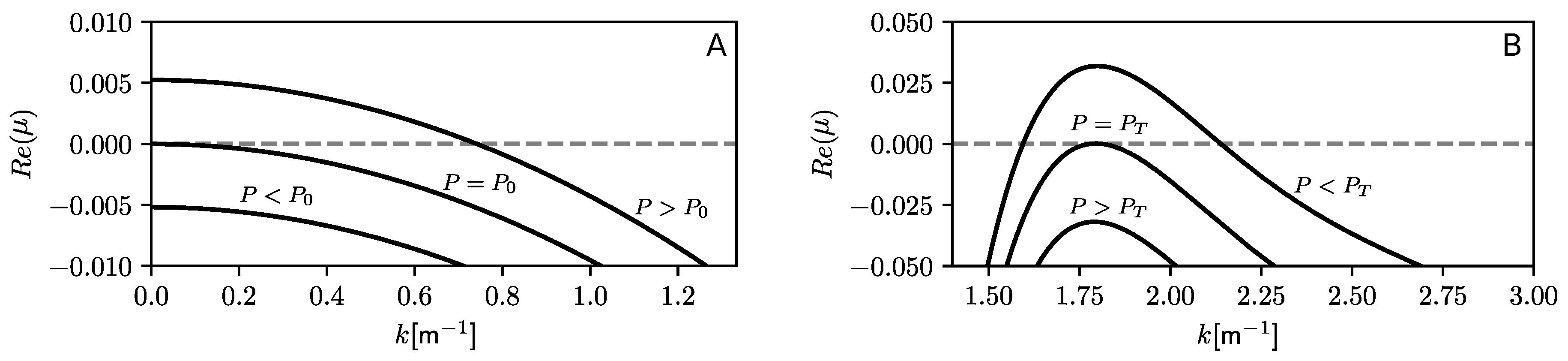
4.1. Instability Thresholds

The simplest solutions of Equation (3) are stationary uniform solutions obtained by solving the algebraic equations that result by setting the time and space derivatives of the state variables to zero. Two such solutions are found, $(B,W)=(0,W_0)$ representing bare soil and existing for all positive precipitation values, P, and $(B,W)=(B_1,W_1)$ representing uniform vegetation and existing only beyond some precipitation threshold (see Figure 4). The stability of these solutions to infinitesimal perturbations of all forms can be calculated using linear stability analysis [11,52]. Such an analysis reveals that the bare-soil state is stable in the precipitation range $0<P<P_0$, where $P_0$ is an instability threshold at which a uniform mode (characterized by zero wavenumber) begins to grow, as the dispersion curves in Figure A1A show. This is a uniform stationary instability [43] where the first mode to grow is spatially uniform and the growth is monotonic in time. Spatial patterning, induced by the root-augmentation feedback or the soil–water diffusion feedback, cannot arise from a nonuniform instability of the bare-soil state as this would involve the growth of a periodic mode from a zero-biomass state and therefore imply negative biomass values, which are unphysical. Failing to obtain a uniform instability of the bare-soil state would indicate a modeling flaw. Such a flaw would be harder to detect in discrete models, such as IBM.

Stationary periodic vegetation patterns may arise from a nonuniform stationary instability of the uniform vegetation state. A linear stability analysis of that state indeed reveals such instability as the precipitation rate P decreases below a threshold value $P_T$. At that threshold a periodic mode with a characteristic wavenumber $k_T$ begins to grow monotonically in time while all other modes still decay, as the dispersion curves in Figure A1B shows. This analysis can be performed even for quite complicated laterally extended root kernels G as shown in Figure 3, see Appendix A. The analysis further confirms the expectation that each of the pattern-forming feedbacks alone, root-augmentation and soil–water diffusion, can induce a nonuniform stationary instability that culminates in stationary periodic patterns.

Linear stability analysis not only unravels possible instabilities and the nature of the modes that grow beyond instability points, but it also provides information about the parameters that control the instability threshold. For example, the instability of the bare-soil state occurs at $P=P_0=MN/\Lambda$, indicating that species with low ratios of growth rates, $\Lambda$, to mortality rates, M, will grow from bare soil at higher precipitation thresholds, or that high evaporation rates, N, act to stabilize the bare soil state. Such relations are less apparent in IBM.

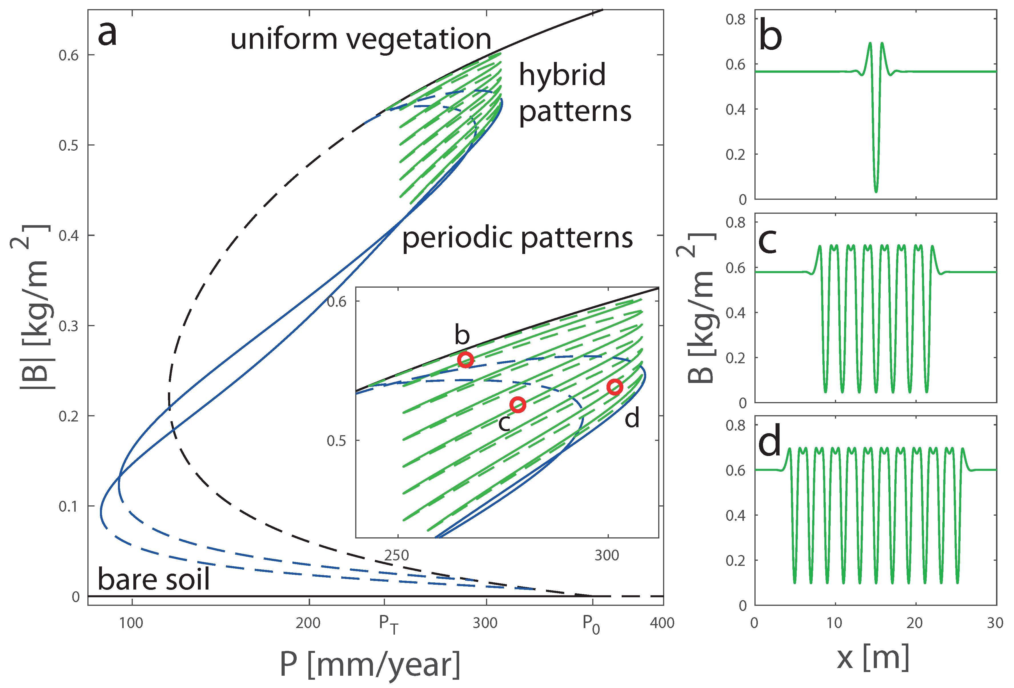
4.2. Bifurcation Diagrams

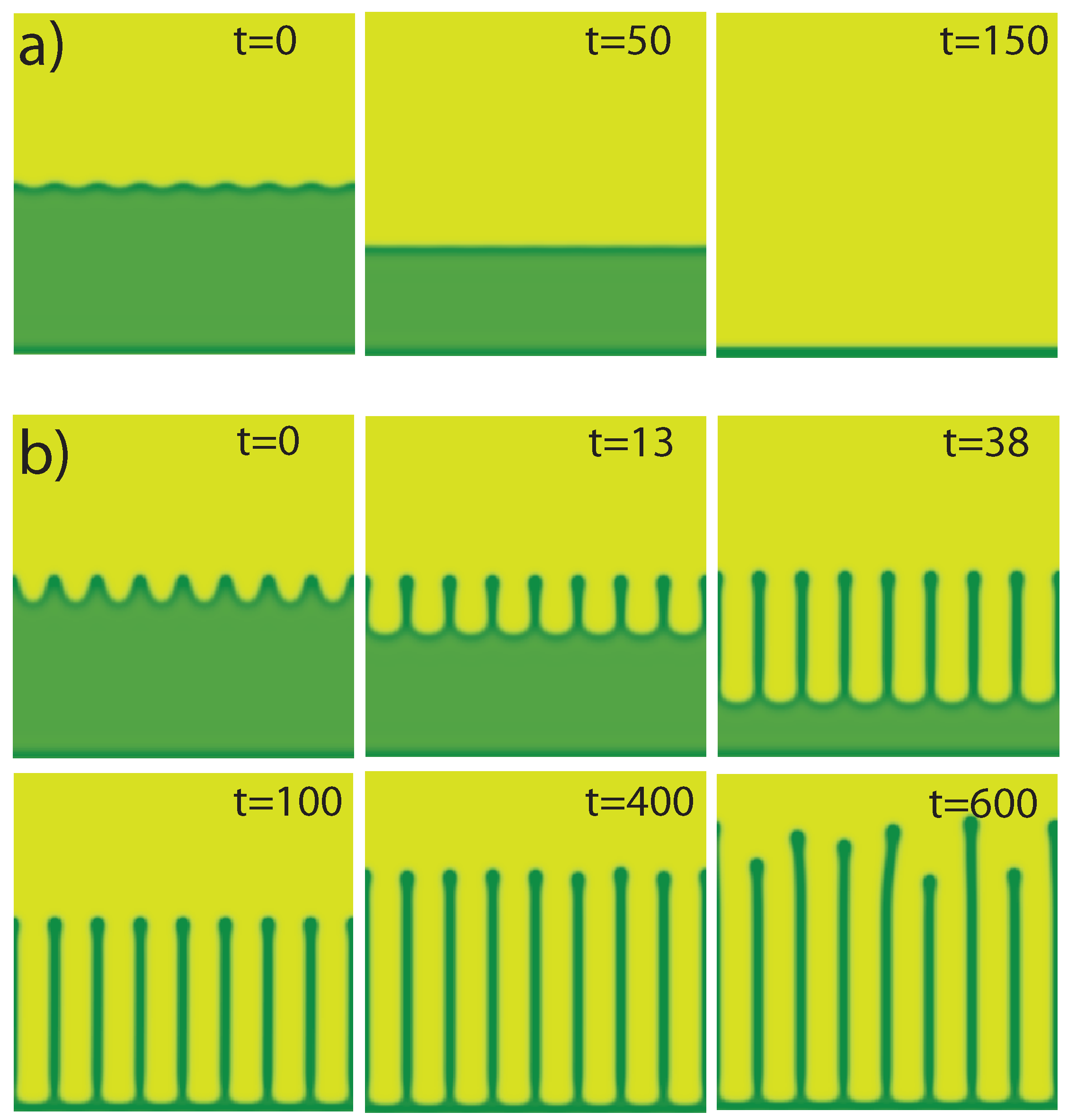
Linear stability analysis does not provide information about the new state that the system converges to following an instability. This kind of information can be obtained by nonlinear analysis of the model equations. A common approach, valid close enough to the instability point, involves the derivation of amplitude equations [11,53,54,55]. These are nonlinear differential equations for the amplitudes of the modes that grow beyond the instability point. Amplitude equations are, in general, much easier to analyze than the original model equations. Moreover, they are dictated by the instability type, rather than by the specific model equations, and therefore are universal; different systems that go through the same instability type (e.g., nonuniform stationary instability) will behave similarly near the instability point. Since all pattern-forming feedbacks lead to the same instability type they will also induce similar dynamics and patterns, although fine details, such as the relative spatial distribution of biomass and water, can reflect differences in the these feedbacks [56].

A convenient way to summarize the outcomes of nonlinear analysis is to draw a bifurcation diagram. Such a diagram shows the existence and stability ranges of various model solutions. In the context of dryland vegetation it often shows graphs of spatial biomass average (or L2 norm) vs. precipitation rate for selected model solutions, using the convention that solid (dashed) lines represent stable (unstable) solutions. If amplitude equations are known, a bifurcation diagram can often be calculated analytically [11,57,58]. When the derivation of amplitude equations is not easy to perform, or when there is an interest in dynamical behaviors far from instability points, bifurcation diagrams can be calculated by numerical continuation methods using software packages such as AUTO [59], pde2path [60], and others. Since these packages solve the equations using iterative solution methods, they converge to unstable solutions as well and, thereby, can provide complete solution branches in the bifurcation diagram.

The utility of bifurcation diagrams can be demonstrated with the example shown in Figure 4, a bifurcation diagram for a vegetation model (see Appendix B) in one space dimension. We focus here on one property that bifurcation diagrams often reveal, namely, parameter ranges where multiple stable states coexist. The (partial) bifurcation diagram of Figure 4 shows a bistability range of bare soil and periodic patterns, a bistability range of bare soil and uniform vegetation, and a tristability subrange of bare soil, periodic patterns and uniform vegetation. The stability of the bare soil state at relative high precipitations values, where uniform vegetation is stable too, can be achieved assuming high evaporation rates (N) in bare soil. Within the tristability range there exists many more stable states, which describe spatial hybrids of periodic pattern and uniform vegetation. These hybrid states appear as confined domains of an increasing size of the patterned state in an otherwise uniform vegetation state, as the insets in Figure 4 show. Hybrid states in bistability ranges of uniform and patterned states have been studied extensively, both mathematically and in particular physical systems. The confined pattern domains are homoclinic solutions that snake back and forth in the bifurcation diagram, a behavior termed “homoclinic snaking” [61,62,63,64,65,66]. They are tightly related to front pinning, that is, to the existence of stationary front solutions between uniform and patterned states over a range of the control parameter. This is in contrast to fronts between distinct uniform states that propagate in general, except, possibly, for a particular parameter value, the so-called Maxwell point at which the fronts are stationary [67,68], and unlike fronts that are pinned by external heterogeneities [69].

Homoclinic snaking has been used to explain fairy-circle dynamics in Namibian grasslands [56,70,71,72]. Fairy circles are circular bare-soil gaps in grasslands that often form nearly periodic hexagonal patterns, where each gap is surrounded by nearly equidistant six other gaps on average [73]. Empirical studies indicate that fairy circles are occasionally “born” or “die” locally [74]. Taking into account the high rainfall inter-annual variability in fairy-circles sites, such dynamical events have been interpreted as transitions between different hybrid states (homoclinic solutions) induced by rainfall fluctuations that are strong enough to drive the ecosystem temporarily outside the existence range of these states (snaking range) [51]. The existence of a multitude of stable hybrid states makes dryland landscapes more plastic in the sense that their response to varying environmental conditions and disturbances can involve temporal convergence to different hybrid states, rather than direct convergence to a single alternative stable state [75].

In order for homoclinic snaking to occur in models of dryland landscapes bistability of uniform vegetation and periodic vegetation patterns are generally sufficient [75,76]. The snaking range in the bifurcation diagram of Figure 4, however, lies within a tristability range of uniform vegetation, periodic pattern and (uniform) bare soil. The existence of that tristability range may have interesting consequences. In particular, the organization of hybrid states within a homoclinic snaking structure can break down as it meets a Maxwell point, where fronts connecting the bare soil and uniform vegetation states are stationary [77]. Another implication of the tristability of two uniform states and a periodic pattern state is the emergence of a family of complex front structures that involve all three states [77].

An additional important aspect that bifurcation diagrams uncover is related to the existence of unstable solution branches. Tracking unstable solutions in bifurcation diagrams can be highly significant when the response of ecosystems to disturbances or human intervention is studied, as the appearance or disappearance of unstable solutions can dramatically affect the flow in phase space and, thus, the response [78]. These subtle aspects, which may have significant ecological implications, become apparent once a bifurcation diagram is calculated. Bifurcation diagrams showing stable and unstable uniform, periodic and localized solutions can be calculated using PDE models [60] but, practically, not with IBM. Bifurcation diagrams have been calculated using IBM but the information they contain is very limited [79,80].

4.3. Front Dynamics

Bistable ecosystems can go through state transitions, or regime shifts [81], in various ways, including a passage through a bifurcation point (B-tipping), as a result of environmental fluctuations (N-tipping), or as a result of fastly varying environmental conditions (R-tipping) [82,83]. Such transitions are generally discussed as whole-system responses, occurring simultaneously at all points in space. Spatially confined disturbances, however, can induce local state transitions. The dynamics that follow such disturbances are dictated by the motion of the fronts that bound the transition area. Of particular interest are degradation fronts, where a dysfunctional state gradually displaces a functional state by front propagation. An example of such a front in the context of dryland vegetation is a desertification front, where a bare-soil domain displaces a vegetated domain [68,84].

PDE models are highly valuable in analyzing desertification fronts and addressing questions such as how to reverse the process of desertification, as we briefly discuss below. We consider again the bifurcation diagram shown in Figure 4, and focus on a bistability precipitation range of bare soil and uniform vegetation, which may or may not include the tristability range where periodic patterns are stable too. In that range we consider precipitation values below the Maxwell point, where desertification fronts exist (bare soil displacing uniform vegetation). In the vicinity of the bare-soil instability to uniform vegetation ($P=P_C$ in Figure 4) the two-variable model presented in Appendix B can be reduced to an amplitude equation for the uniform mode that begins to grow at this instability [85]. Analysis of this equation reveals a transverse front instability [86,87], whereby small bulges along the front line are first enhanced, then develop into growing fingers that avoid one another, and ultimately fill up the system domain with a stationary labyrinthine pattern.

According to the analysis of the amplitude equation, the instability occurs as the soil–water diffusion coefficient, $D_W$, exceeds a threshold value, and that threshold is inversely related to the root-to-shoot ratio, E, which controls water uptake by plants’ roots [85]. This result uncovers the mechanism of the instability—fast soil–water diffusion (relative to biomass expansion) towards incidental bulges along the front line that locally deplete the soil–water content. The fast diffusion acts to enhance the growth of these bulges and, at the same time, to inhibit vegetation growth on both sides of any bulge. Fast diffusion can be obtained by increasing the diffusion coefficient, $D_W$, which is consistent with the finding of a threshold value above which the instability develops. Fast diffusion is also obtained by steepening the soil–water gradients, which can be achieved by strong water uptake. This is consistent with the finding that the threshold value decreases as the parameter E that controls water uptake, is increased.

Figure 5 shows a desertification front that develops a transverse instability. While the bare soil area initially expands into the vegetated area, the instability results in vegetation fingers that grow backward into the bare-soil area and thereby reverse the desertification process. The resulting state is a productive vegetation pattern that prevents further irreversible degradation processes (not captured by the model), such as soil erosion, and maintains the ecosystem in a reversible state capable of forming uniform vegetation when favorable rainfall conditions resume. But how can a transverse instability be induced in stable desertification fronts? One possible answer to this question is the introduction of a species with sufficiently high root-to-shoot ratio so as to reduce the threshold value of $D_W$ above which the instability sets in, and thereby induce a transverse instability. There is, however, another possibility associated with the tristability range of uniform vegetation, bare soil and periodic patterns. In this range, desertification fronts that are stable to small perturbations (linearly stable) may still be unstable to larger perturbations (nonlinearly unstable), which drive the system to the periodic-pattern state through finger growth [88] as Figure 6 demonstrates.

These results are very appealing from the point of view of ecosystem management. First, they imply local manipulations in the front zone only, rather than extensive intervention across the whole ecosystem. The manipulations may involve planting a different species capable of inducing a linear front instability, or modulating the front line strongly enough in order to induce a nonlinear front instability. The latter intervention form may involve periodic grazing management, clear-cutting or irrigation, and is relevant in cases when indications for the existence of periodic patterns exist (e.g., scattered patches of periodic vegetation). Second, such manipulations are limited in time, as they are needed only to trigger the instability. Once the instability sets in, a process of self-recovery begins. These conclusions, which are based on the mathematical analysis of front solutions, could not have been obtained in studies of IBM.

5. Discussion

Despite their typically small size, discrete plant populations in dryland ecosystems can still be described by continuum PDE models because of the high phenotypic plasticity of plants and the dispersal of stress-tolerant seeds, as discussed in Section 2 and Section 3. Since the state variables that describe plant population sizes should reflect that plasticity, biomass densities are more appropriate choices for plant populations than the often used number densities in population dynamics studies. Unlike IBM, where the smallest entity is a single individual, in PDE models with biomass densities as state variables, the smallest entity is a small area element and the processes that take place there. That area element can be significantly smaller than the scale of a single plant and its roots.

We presented here several examples that demonstrate the utility of continuum PDE models in gaining mechanistic information and insights about large, landscape-scale behaviors, such as the onset of a nonuniform stationary instability that culminates in periodic vegetation patterns, uncovering precipitation ranges of bistability, tristability and multistability of uniform states, periodic patterns and localized patterns (hybrid states), and dynamics of desertification fronts, where we focused on front instabilities that may reverse gradual desertification. Many more examples exist, a few of them are briefly discussed below.

On a slope, a linear stability analysis of uniform vegetation has revealed a nonuniform oscillatory instability that results in traveling-wave solutions. These solutions describe periodic vegetation stripes migrating uphill [89,90], as observed in empirical studies [91]. The migration mechanism is easy to understand; while plants at the top part of a vegetation stripe receive runoff and grow, plants at the bottom part loose runoff and die. PDE models have been instrumental in clarifying the relations between migration speed, pattern wavelength, and slope [92,93].

Studies of PDE models in one space dimension have identified many periodic solutions along the rainfall gradient, the wavenumbers of which decrease as precipitation decreases, down to zero in a solution that represents a single vegetation patch [94,95,96]. These solutions reflect two manners by which patchy vegetation responds to water stress. The first is an increase of bare soil areas at the expense of vegetation-patch areas, keeping the wavenumber unchanged. This response occurs along each solution branch [97]. The second response is a transition to a periodic solution with a lower wavenumber, quite often half the original wavenumber [95,96,97]. In this response, the area of each vegetation patch does not necessarily decrease, but the number of vegetation patches decreases. In both response forms, the increase in bare-soil area compensates for the reduced rainfall through increased water transport to adjacent vegetation patches by one of the transport mechanisms discussed in Section 3.1. Empirical indications for the existence of periodic patterns with different wavenumbers have been found in studies of banded vegetation in Somalia [98].

In two space dimensions, patchy vegetation can respond to water stress by yet another mechanism of increasing bare-soil areas, namely, morphological changes, first from hexagonal gap patterns to stripe patterns, and, at lower precipitation, from stripe patterns to hexagonal spot patterns [36,43,99]. In cases where the instability of bare soil to uniform vegetation is supercritical, weak nonlinear analyses of PDE models in two space dimensions have produced bifurcation diagrams that unfold the basic periodic vegetation patterns along the rainfall gradient: hexagonal gap patterns, stripe patterns and hexagonal spot patterns [57,58]. Empirical indications for the existence of these vegetation patterns in nature are abundant, although not yet with a single plant species along a rainfall gradient [56,73,100,101,102].

PDE models have also been used to study the interactions between two distinct plant species. One interesting context of such interactions is the bistability of a uniform state of one species and a periodic-pattern state of the other species. In this range, homoclinic snaking can result in the multistability of hybrid states that involve the two species, and therefore constitutes a mechanism for species coexistence [103]. Another interesting context is woody-herbaceous systems, where the woody species is pattern forming. Studies of a PDE model that captures both the infiltration feedback and the root-augmentation feedback reveal changes in the relative importance of the two feedbacks along the rainfall gradient. At high precipitation dominance of the root augmentation feedback results in a strong depletion of the soil–water content and the exclusion of herbaceous vegetation. At low precipitation, the dominance of the infiltration feedback results in soil–water concentration at woody patches and the consequent facilitation of herbaceous-vegetation growth [41]. These results are consistent with the stress-gradient hypothesis in ecology [104].

While these results are hard to obtain using IBM, we should not regard PDE models as substitutes to IBM, but rather as complementary means to gain deeper mechanistic understanding. IBM typically go into much more details, and attempts to include these details in PDE models would render them mathematically intractable too. PDE models should rather be motivated by specific questions of interest and by judicious assessments of the processes that are most relevant to these questions. The vegetation models described in Section 3 have been motivated by empirical observations of regular vegetation patterns in drylands and by the understanding that the most relevant processes to these phenomena are positive feedback loops involving vegetation growth and water availability that can induce pattern-forming instabilities. Various other processes, considered to be of secondary significance, have been left aside, such as the effect of transpiration on the atmosphere, soil erosion and deposition, and various plant physiology processes. Such processes are likely to have quantitative rather than qualitative effects on vegetation pattern formation; they may affect, for example, instability thresholds, but are not likely to affect the occurrence of instabilities or change their nature. While providing deep mechanistic insights into ecological processes, and predicting possible qualitative responses to environmental changes, PDE models should not be regarded as tools for making quantitative forecasts.

References

1. Hansen, J.; Sato, M.; Ruedy, R. Perception of climate change. Proc. Natl. Acad. Sci. USA 2012, 109, E2415–E2423. [Google Scholar] [CrossRef] [PubMed] [Green Version]
2. Hoerling, M.; Eischeid, J.; Perlwitz, J.; Quan, X.; Zhang, T.; Pegion, P. On the Increased Frequency of Mediterranean Drought. J. Clim. 2012, 25, 2146–2161. [Google Scholar] [CrossRef] [Green Version]
3. Cook, B.I.; Ault, T.R.; Smerdon, J.E. Unprecedented 21st century drought risk in the American Southwest and Central Plains. Sci. Adv. 2015, 1, e1400082. [Google Scholar] [CrossRef] [PubMed] [Green Version]
4. DeAngelis, D.; Grimm, V. Individual-based models in ecology after four decades. F1000Prime 2014, 6, 39. [Google Scholar] [CrossRef] [PubMed] [Green Version]
5. Grimm, V.; Railsback, S.F. Individual-Based Modeling and Ecology; Princeton University Press: Princeton, NJ, USA, 2005. [Google Scholar]
6. DeAngelis, D.L.; Yurek, S. Spatially Explicit Modeling in Ecology: A Review. Ecosystems 2016. [Google Scholar] [CrossRef]
7. Holmes, E.E.; Lewis, M.A.; Banks, J.E.; Veit, R.R. Partial Differential Equations in Ecology: Spatial Interactions and Population Dynamics. Ecology 1994, 75, 17–29. [Google Scholar] [CrossRef]
8. Petrovskii, S.V.; Li, B.L. Exactly Solvable Models of Biological Invasion; Chapman and Hall/CRC Mathematical and Computational Biology; CRC Press: Boca Raton, FL, USA, 2005. [Google Scholar]
9. Petrovskii, S.V.; Morozov, A.Y.; Venturino, E. Allee effect makes possible patchy invasion in a predator–prey system. Ecol. Lett. 2002, 5, 345–352. [Google Scholar] [CrossRef]
10. Cantrell, R.S.; Cosner, C. Spatial Ecology via Reaction-Diffusion Equations; Wiley Series in Mathematical & Computational Biology; Wiley: San Francisco, CA, USA, 2003. [Google Scholar]
11. Meron, E. Nonlinear Physics of Ecosystems; CRC Press, Taylor & Francis Group: Boca Raton, FL, USA, 2015. [Google Scholar]
12. Ovaskainen, O.; Meerson, B. Stochastic models of population extinction. Trends Ecol. Evol. 2010, 25, 643–652. [Google Scholar] [CrossRef] [Green Version]
13. Bonachela, J.A.; Muñoz, M.A.; Levin, S.A. Patchiness and demographic noise in three ecological examples. J. Stat. Phys. 2012, 148, 723–739. [Google Scholar] [CrossRef]
14. Pigliucci, M. Evolution of phenotypic plasticity: Where are we going now? Trends Ecol. Evol. 2005, 20, 481–486. [Google Scholar] [CrossRef]
15. Aichinger, E.; Kornet, N.; Friedrich, T.; Laux, T. Plant stem cell niches. Annu. Rev. Plant Biol. 2012, 63, 615–636. [Google Scholar] [CrossRef] [PubMed]
16. Mokany, K.; Raison, J.; Prokushkin, A. Critical analysis of root-shoot rations in terrestrial biomes. Glob. Chang. Biol. 2006, 12, 84–96. [Google Scholar] [CrossRef]
17. Khadka, J.; Yadav, N.; Granot, G.; Grafi, G. Summer dormancy is associated with loss of the permissive epigenetic marker dimethyl H3K4 and extensive reduction in proteins involved in basic cell functions. Plants 2018, 7, 59. [Google Scholar] [CrossRef] [PubMed]
18. Grafi, G. A “mille-feuilles” of stress tolerance in the desert plant Zygophyllum dumosum Boiss. Isr. J. Plant Sci. 2019, 66, 52–59. [Google Scholar] [CrossRef]
19. Evenari, M.; Shanan, L.; Tadmor, N. The Negev: The Challenge of a Desert; Harvard University Press: Cambridge, MA, USA, 1982. [Google Scholar]
20. Terwilliger, V.; Zeroni, M. Gas exchange of a desert shrub (Zygophyllum dumosum Boiss.) under different soil moisture regimes during summer drought. J. Plant Ecol. 1994, 115, 133–144. [Google Scholar]
21. Schenk, J.H.; Espino, S.; Goedhart, C.M.; Nordenstahl, M.; Cabrera, H.I.; Jones, C.S. Hydraulic integration and shrub growth form linked across continental aridity gradients. Proc. Natl. Acad. Sci. USA 2008, 105, 11248–11253. [Google Scholar] [CrossRef] [PubMed] [Green Version]
22. Ginzburg, C. Some anatomic features of splitting of desert shrubs. Annu. Rev. Plant Biol. 1963, 13, 92–97. [Google Scholar]
23. Orshan, G.; Zand, G. Seasonal body reduction of certain desert halfshrubs. Bull. Res. Counc. Isr. 1962, 11D, 35–42. [Google Scholar]
24. Cunningham, G.; Strain, B. An ecological significance of seasonal leaf variability in a desert shrub. Ecology 1969, 50, 400–408. [Google Scholar] [CrossRef]
25. Dalling, J.; Davis, A.; Schutte, B.; Elizabeth, A.A. Seed survival in soil: Interacting effects of predation, dormancy and the soil microbial community. J. Ecol. 2011, 99, 89–95. [Google Scholar] [CrossRef]
26. Kivilaan, A.; Bandurski, R. The one hundred-year period for Dr. Beal’s seed viability experiment. Am. J. Bot. 1981, 68, 1290–1292. [Google Scholar] [CrossRef]
27. Shen-Miller, J.; Mudgett, M.; Schopf, J.; Clarke, S.; Berger, R. Exceptional seed longevity and robust growth: Ancient sacred lotus from China. Am. J. Bot. 1995, 82, 1367–1380. [Google Scholar] [CrossRef]
28. Long, R.; Gorecki, M.; Renton, M.; Scott, J.; Colville, L.; Goggin, D.; Commander, L.; Westcott, D.; Cherry, H.; Finch-Savage, W. The ecophysiology of seed persistence: A mechanistic view of the journey to germination or demise. Biol. Rev. Camb. Philos. Soc. 2015, 90, 31–59. [Google Scholar] [CrossRef] [PubMed]
29. Cohen, D. A general model of optimal reproduction in a randomly varying environment. Am. J. Bot. 1966, 56, 219–228. [Google Scholar] [CrossRef]
30. Venable, D.; Brown, J. The selective interactions of dispersal, dormancy, and seed size as adaptations for reducing risk in variable environments. Am. Nat. 1988, 131, 360–384. [Google Scholar] [CrossRef]
31. Ooi, M. Seed bank persistence and climate change. Seed Sci. Res. 2012, 22, S53–S60. [Google Scholar] [CrossRef] [Green Version]
32. Walck, J.; Hidayati, S.; Dixon, K.; Thompson, K.; Poschlod, P. Climate change and plant regeneration from seed. Glob. Chang. Biol. 2011, 17, 2145–2161. [Google Scholar] [CrossRef]
33. Raviv, B.; Godwin, J.; Granot, G.; Grafi, G. The dead can nurture: Novel insights into the function of dead organs enclosing embryos. Int. J. Mol. Sci. 2018, 19, 2455. [Google Scholar] [CrossRef]
34. Lefever, R.; Lejeune, O. On the origin of tiger bush. Bull. Math. Biol. 1997, 59, 263–294. [Google Scholar] [CrossRef]
35. Klausmeier, C. Regular and irregular patterns in semiarid vegetation. Science 1999, 284, 1826–1828. [Google Scholar] [CrossRef]
36. Von Hardenberg, J.; Meron, E.; Shachak, M.; Zarmi, Y. Diversity of Vegitation Patterns and Desertification. Phys. Rev. Lett. 2001, 87, 198101. [Google Scholar] [CrossRef] [PubMed]
37. Shnerb, N.; Sarah, P.; Lavee, H.; Solomon, S. Reactive glass and vegetation patterns. Phys. Rev. Lett. 2003, 90, 0381011. [Google Scholar] [CrossRef] [PubMed]
38. HilleRisLambers, R.; Rietkerk, M.; Van den Bosch, F.; Prins, H.; de Kroon, H. Vegetation pattern formation in semi-arid grazing systems. Ecology 2001, 82, 50–61. [Google Scholar] [CrossRef]
39. Gilad, E.; Von Hardenberg, J.; Provenzale, A.; Shachak, M.; Meron, E. Ecosystem Engineers: From Pattern Formation to Habitat Creation. Phys. Rev. Lett. 2004, 93, 098105. [Google Scholar] [CrossRef] [PubMed]
40. Gilad, E.; Von Hardenberg, J.; Provenzale, A.; Shachak, M.; Meron, E. A Mathematical Model for Plants as Ecosystem Engineers. J. Theor. Biol. 2007, 244, 680. [Google Scholar] [CrossRef]
41. Gilad, E.; Shachak, M.; Meron, E. Dynamics and Spatial Organization of Plant Communities in Water Limited Systems. Theor. Popul. Biol. 2007, 72, 214–230. [Google Scholar] [CrossRef] [PubMed]
42. Kinast, S.; Zelnik, Y.R.; Bel, G.; Meron, E. Interplay between Turing Mechanisms can Increase Pattern Diversity. Phys. Rev. Lett. 2014, 112, 078701. [Google Scholar] [CrossRef] [Green Version]
43. Meron, E. From Patterns to Function in Living Systems: Dryland Ecosystems as a Case Study. Annu. Rev. Condens. Matter Phys. 2018, 9, 79–103. [Google Scholar] [CrossRef]
44. Meron, E. Pattern formation—A missing link in the study of ecosystem response to environmental changes. Math. Biosci. 2016, 271, 1–18. [Google Scholar] [CrossRef]
45. Meinhardt, H. Pattern formation in biology: A comparison of models and experiments. Rep. Prog. Phys. 1992, 55, 797. [Google Scholar] [CrossRef]
46. Rietkerk, M.; van de Koppel, J. Regular pattern formation in real ecosystems. Trends Ecol. Evol. 2008, 23, 169–175. [Google Scholar] [CrossRef] [PubMed]
47. Verrecchia, E.; Yair, A.; Kidron, G.J.; Verrecchia, K. Physical properties of the psammophile cryptogamic crust and their consequences to the water regime of sandy softs, north-western Negev Desert, Israel. J. Arid Environ. 1995, 29, 427–437. [Google Scholar] [CrossRef]
48. Eldridge, D.J.; Zaady, E.; Shachak, M. Infiltration through three contrasting biological soil crusts in patterned landscapes in the Negev, Israel. J. Stat. Phys. 2012, 148, 723–739. [Google Scholar] [CrossRef]
49. Walker, B.; Ludwig, D.; Holling, C.; Peterman, R. Stability of semi-arid savana grazing systems. J. Ecol. 1981, 69, 473–498. [Google Scholar] [CrossRef]
50. Atkinson, J.A.; Rasmussen, A.; Traini, R.; Voß, U.; Sturrock, C.; Mooney, S.; Wells, D.M.; Bennett, M.J. Branching Out in Roots: Uncovering Form, Function, and Regulation. Plant Physiol. 2014, 166, 538–550. [Google Scholar] [CrossRef] [PubMed] [Green Version]
51. Zelnik, Y.R.; Meron, E.; Bel, G. Gradual Regime Shifts in Fairy Circles. Proc. Natl. Acad. Sci. USA 2015, 112, 12327–12331. [Google Scholar] [CrossRef]
52. Strogatz, S.H. Nonlinear Dynamics and Chaos: With Applications to Physics, Biology, Chemistry, and Engineering; Westview Press: Pittsburgh, PA, USA, 2001. [Google Scholar]
53. Newell, A.C.; Passot, T.; Lega, J. Order parameter equations for patterns. Ann. Rev. Fluid Mech. 1993, 25, 399–453. [Google Scholar] [CrossRef]
54. Elphick, C.; Tirapegui, E.; Brachet, M.E.; Coullet, P.; Iooss, G. A simple global characterization for normal forms of singular vector fields. Phys. D 1987, 29, 95–127. [Google Scholar] [CrossRef]
55. Cross, M.; Greenside, H. Pattern Formation and Dynamics in Nonequilibrium Systems; Cambridge University Press: Cambridge, UK, 2009. [Google Scholar]
56. Getzin, S.; Yizhaq, H.; Bell, B.; Erickson, T.E.; Postle, A.C.; Katra, I.; Tzuk, O.; Zelnik, Y.R.; Wiegand, K.; Wiegand, T.; et al. Discovery of fairy circles in Australia supports self-organization theory. Proc. Natl. Acad. Sci. USA 2016, 113, 3551–3556. [Google Scholar] [CrossRef] [Green Version]
57. Lejeune, O.; Tlidi, M.; Lefever, R. Vegetation spots and stripes: Dissipative structures in arid landscapes. Int. J. Quantum Chem. 2004, 98, 261–271. [Google Scholar] [CrossRef]
58. Gowda, K.; Riecke, H.; Silber, M. Transitions between patterned states in vegetation models for semiarid ecosystems. Phys. Rev. E 2014, 89, 022701. [Google Scholar] [CrossRef] [PubMed] [Green Version]
59. Doedel, E.; Paffenroth, R.C.; Champneys, A.R.; Fairgrieve, T.F.; Kuznetsov, Y.A.; Oldeman, B.E.; Sandstede, B.; Wang, X. AUTO2000; Technical report; Concordia University: Montréal, QC, Canada, 2002. [Google Scholar]
60. Uecker, H.; Wetzel, D.; Rademacher, J.D. pde2path-A Matlab package for continuation and bifurcation in 2D elliptic systems. Numer. Math. Theory Methods Appl. 2014, 7, 58–106. [Google Scholar] [CrossRef]
61. Kozyreff, G.; Chapman, S.J. Asymptotics of Large Bound States of Localized Structures. Phys. Rev. Lett. 2006, 97, 044502. [Google Scholar] [CrossRef] [PubMed] [Green Version]
62. Burke, J.; Knobloch, E. Snakes and ladders: Localized states in the Swift-Hohenberg equation. Phys. Lett. A 2007, 360, 681–688. [Google Scholar] [CrossRef]
63. Dawes, J. Localized Pattern Formation with a Large-Scale Mode: Slanted Snaking. SIAM J. Appl. Dyn. Syst. 2008, 7, 186–206. [Google Scholar] [CrossRef] [Green Version]
64. Lloyd, D.J.B.; Sandstede, B.; Avitabile, D.; Champneys, A.R. Localized Hexagon Patterns of the Planar Swift-Hohenberg Equation. SIAM J. Appl. Dyn. Syst. 2008, 7, 1049–1100. [Google Scholar] [CrossRef]
65. Avitabile, D.; Lloyd, D.; Burke, J.; Knobloch, E.; Sandstede, B. To Snake or Not to Snake in the Planar Swift–Hohenberg Equation. SIAM J. Appl. Dyn. Syst. 2010, 9, 704–733. [Google Scholar] [CrossRef]
66. Knobloch, E. Spatial Localization in Dissipative Systems. Annu. Rev. Condens. Matter Phys. 2015, 6, 325–359. [Google Scholar] [CrossRef] [Green Version]
67. Pomeau, Y. Front motion, metastability and subcritical bifurcations in hydrodynamics. Physica D 1986, 23, 3. [Google Scholar] [CrossRef]
68. Bel, G.; Hagberg, A.; Meron, E. Gradual regime shifts in spatially extended ecosystems. Theor. Ecol. 2012, 5, 591–604. [Google Scholar] [CrossRef] [Green Version]
69. Clerc, M.G.; Fernandez-Oto, C.; García-Ñustes, M.A.; Louvergneaux, E. Origin of the Pinning of Drifting Monostable Patterns. Phys. Rev. Lett. 2012, 109, 104101. [Google Scholar] [CrossRef] [PubMed] [Green Version]
70. Juergens, N. The biological underpinnings of Namib Desert fairy circles. Science 2013, 339, 1618–1621. [Google Scholar] [CrossRef] [PubMed]
71. Fernandez-Oto, C.; Tlidi, M.; Escaff, D.; Clerc, M.G. Strong interaction between plants induces circular barren patches: Fairy circles. Philos. Trans. A Math. Phys. Eng. Sci. 2014, 372, 20140009. [Google Scholar] [CrossRef] [PubMed]
72. Tarnita, C.; Bonachela, J.A.; Sheffer, E.; Guyton, J.A.; Coverdale, T.C.; Long, R.A.; Pringle, R.M. A theoretical foundation for multi-scale regular vegetation patterns. Nature 2017, 541, 398–401. [Google Scholar] [CrossRef] [PubMed] [Green Version]
73. Getzin, S.; Wiegand, K.; Wiegand, T.; Yizhaq, H.; von Hardenberg, J.; Meron, E. Adopting a spatially explicit perspective to study the mysterious fairy circles of Namibia. Ecography 2015, 38, 1–11. [Google Scholar] [CrossRef]
74. Tschinkel, W. The Life Cycle and Life Span of Namibian Fairy Circles. PLoS ONE 2012, 7, e38056. [Google Scholar] [CrossRef]
75. Zelnik, Y.R.; Meron, E.; Bel, G. Localized states qualitatively change the response of ecosystems to varying conditions and local disturbances. Ecol. Complex. 2016, 25, 26–34. [Google Scholar] [CrossRef] [Green Version]
76. Dawes, J.; Williams, J. Localised pattern formation in a model for dryland vegetation. J. Math. Biol. 2016, 73, 63–90. [Google Scholar] [CrossRef]
77. Zelnik, Y.R.; Gandhi, P.; Knobloch, E.; Meron, E. Implications of tristability in pattern-forming ecosystems. Chaos Interdiscip. J. Nonlinear Sci. 2018, 28, 033609. [Google Scholar] [CrossRef]
78. Mau, Y.; Haim, L.; Meron, E. Reversing desertification as a spatial resonance problem. Phys. Rev. E 2015, 91, 012903. [Google Scholar] [CrossRef] [Green Version]
79. Xu, C.; Van Nes, E.H.; Holmgren, M.; Kéfi, S.; Scheffer, M. Local Facilitation May Cause Tipping Points on a Landscape Level Preceded by Early-Warning Indicators. Am. Nat. 2015, 186, E81–E90. [Google Scholar] [CrossRef] [PubMed]
80. Van Strien, M.J.; Huber, S.H.; Anderies, J.M.; Grêt-Regamey, A. Resilience in social-ecological systems: Identifying stable and unstable equilibria with agent-based models. Ecol. Soc. 2019, 24, 8. [Google Scholar] [CrossRef]
81. Scheffer, M.; Carpenter, S.; Foley, J.; Folke, C.; Walkerk, B. Catastrophic shifts in ecosystems. Nature 2001, 413, 591–596. [Google Scholar] [CrossRef] [PubMed]
82. Ashwin, P.; Wieczorek, S.; Vitolo, R.; Cox, P. Tipping points in open systems: Bifurcation, noise-induced and rate-dependent examples in the climate system. Philos. Trans. Math. Phys. Eng. Sci. 2012, 370, 1166–1184. [Google Scholar] [CrossRef] [PubMed]
83. Feudel, U.; Pisarchik, A.N.; Showalter, K. Multistability and tipping: From mathematics and physics to climate and brain—Minireview and preface to the focus issue. Chaos Interdiscip. J. Nonlinear Sci. 2018, 28, 033501. [Google Scholar] [CrossRef] [PubMed]
84. Zelnik, Y.R.; Meron, E. Regime shifts by front dynamics. Ecol. Indic. 2018, 94, 544–552. [Google Scholar] [CrossRef]
85. Fernandez-Oto, C.; Tzuk, O.; Meron, E. Front Instabilities Can Reverse Desertification. Phys. Rev. Lett. 2019, 122, 048101. [Google Scholar] [CrossRef] [Green Version]
86. Hagberg, A.; Meron, E. Complex Patterns in reaction Diffusion Systems: A Tale of Two Front Instabilities. Chaos 1994, 4, 477–484. [Google Scholar] [CrossRef]
87. Goldstein, R.E.; Muraki, D.J.; Petrich, D.M. Interface proliferation and the growth of labyrinths in a reaction-diffusion system. Phys. Rev. E 1996, 53, 3933–3957. [Google Scholar] [CrossRef] [Green Version]
88. Hagberg, A.; Yochelis, A.; Yizhaq, H.; Elphick, C.; Pismen, L.; Meron, E. Linear and nonlinear front instabilities in bistable systems. Phys. D Nonlinear Phenom. 2006, 217, 186–192. [Google Scholar] [CrossRef]
89. Ursino, N. The influence of soil properties on the formation of unstable vegetation patterns on hillsides of semiarid catchments. Adv. Water Resour. 2005, 28, 956–963. [Google Scholar] [CrossRef]
90. Sherratt, J.A. An Analysis of Vegetation Stripe Formation in Semi-Arid Landscapes. J. Math. Biol. 2005, 51, 183–197. [Google Scholar] [CrossRef] [PubMed]
91. Deblauwe, V.; Couteron, P.; Bogaert, J.; Barbier, N. Determinants and dynamics of banded vegetation pattern migration in arid climates. Ecol. Monogr. 2012, 82, 3–21. [Google Scholar] [CrossRef] [Green Version]
92. Sherratt, J.A. Pattern Solutions of the Klausmeier Model for Banded Vegetation in Semiarid Environments V: The Transition from Patterns to Desert. SIAM J. Appl. Math. 2013, 73, 1347–1367. [Google Scholar] [CrossRef]
93. Sherratt, J.A. Using wavelength and slope to infer the historical origin of semiarid vegetation bands. Proc. Natl. Acad. Sci. USA 2015, 112, 4202–4207. [Google Scholar] [CrossRef] [Green Version]
94. Sherratt, J.A.; Lord, G.J. Nonlinear dynamics and pattern bifurcations in a model for vegetation stripes in semi-arid environments. Theor. Popul. Biol. 2007, 71, 1–11. [Google Scholar] [CrossRef]
95. Zelnik, Y.R.; Kinast, S.; Yizhaq, H.; Bel, G.; Meron, E. Regime shifts in models of dryland vegetation. Philos. Trans. R. Soc. A 2013, 371, 20120358. [Google Scholar] [CrossRef]
96. Siteur, K.; Siero, E.; Eppinga, M.B.; Rademacher, J.D.M.; Doelman, A.; Rietkerk, M. Beyond Turing: The response of patterned ecosystems to environmental change. Ecol. Complex. 2014, 20, 81–96. [Google Scholar] [CrossRef]
97. Yizhaq, H.; Gilad, E.; Meron, E. Banded Vegetation: Biological Productivity and Resilience. Physica A 2005, 356, 139. [Google Scholar] [CrossRef]
98. Bastiaansen, R.; Jaïbi, O.; Deblauwe, V.; Eppinga, M.B.; Siteur, K.; Siero, E.; Mermoz, S.; Bouvet, A.; Doelman, A.; Rietkerk, M. Multistability of model and real dryland ecosystems through spatial self-organization. Proc. Natl. Acad. Sci. USA 2018, 115, 11256–11261. [Google Scholar] [CrossRef] [Green Version]
99. Rietkerk, M.; Dekker, S.C.; de Ruiter, P.C.; van de Koppel, J. Self-Organized Patchiness and Catastrophic Shifts in Ecosystems. Science 2004, 305, 1926–1929. [Google Scholar] [CrossRef] [PubMed] [Green Version]
100. Valentine, C.; d’Herbes, J.; Poesen, J. Soil and water components of banded vegetation patterns. Catena 1999, 37, 1–24. [Google Scholar] [CrossRef]
101. Deblauwe, V.; Barbier, N.; Couteron, P.; Lejeune, O.; Bogaert, J. The global biogeography of semi-arid periodic vegetation patterns. Glob. Ecol. Biogeogr. 2008, 17, 715–723. [Google Scholar] [CrossRef]
102. Borgogno, F.; D’Odorico, P.; Laio, F.; Ridolfi, L. Mathematical models of vegetation pattern formation in ecohydrology. Rev. Geophys. 2009, 47, RG1005. [Google Scholar] [CrossRef]
103. Kyriazopoulos, P.; Jonathan, N.; Meron, E. Species coexistence by front pinning. Ecol. Complex. 2014, 20, 271–281. [Google Scholar] [CrossRef]
104. Malkinson, D.; Tielbörger, K. What does the stress-gradient hypothesis predict? Resolving the discrepancies. Oikos 2010, 119, 1546–1552. [Google Scholar] [CrossRef]
Figure 1. Phenology of Zygophyllum dumosum Boiss growing on a southeast-facing slope at Sede Boqer research area (30o 51 N 34o 46 E; elevation 498 m). (A) A typical branch of Zygophyllum plant during the wet season (March 2008). Note the coumpond leaf composed of two leaflets (LL) carried on a fleshy, cylindrical petiole (P). 1YOP, 1-year-old petiole. (B) A typical Z. dumosum branch during the dry season carrying petioles (P). (C) A closer look at emerging new bud from the axil of a 1YOP at the beginning of the winter. (D) Axis splitting resulting in a dual appearance of a Z. dumosum plant showing healthy branches carrying new leaves and flowers (right from the broken line) and unhealthy branches (left from the broken line). (E) A Z. dumosum plant with the main axis divided into several distinct units.
Mathematics 07 00987 g001
Figure 2. A general positive feedback loop that drives the formation of vegetation patterns in drylands. The feedback concomitantly accelerates vegetation growth in patches of denser vegetation and inhibits the growth in adjacent sparser patches. The combined processes favor the growth of nonuniform perturbations and the formation of vegetation patterns. From [11].
Mathematics 07 00987 g002
Figure 3. Root system growth as shoot biomass increases. A plot of the axisymmetric root kernel, G (see (A1) in Appendix A), as a function of the space coordinate X when (A) B ( X , T ) = 0 , (B) B ( X , T ) = 0.2 , (C) B ( X , T ) = 0.3 , (D) B ( X , T ) = 0.4 = : K . The kernel is a Gaussian function multiplied by a polynomial factor, that mimics adventitious root branching observed in some plant species [50]. Parameters in (A1) and (A2): S 0 = 0.15 m, c 0 = 1 , c 2 = 0.135 , c 4 = 7.09 × 10 3 , c 6 = 9.11 × 10 5 , c 8 = 3.84 × 10 7 .
Mathematics 07 00987 g003
Figure 4. Bifurcation diagram for the model presented in Appendix B (Equation (A17)) in 1D (panel a). The vertical axis is the spatial biomass average, while the horizontal axis is the precipitation rate. Solid (dashed) lines represent stable (unstable) solutions. The diagram shows bistability precipitation ranges of bare soil and periodic patterns, and of bare soil and uniform vegetation, as well as a tristability range of bare soil, uniform vegetation and periodic patterns. Within the latter range there exists a subrange of hybrid patterns, consisting of confined pattern domains of increasing size in an otherwise uniform vegetation, examples of which are shown in the three panels (bd). Parameters: Λ = 0.1 [(m 2 /kg)/y], Γ = 4 [(m 2 /kg)/y], E = 7 [m 2 /kg], K = 1 [kg/m 2 ], M = 4.5 [1/y], N = 8 [1/y], R = 0.1 , D B = 0.05 [m 2 /y], D W = 30 [m 2 /y].
Mathematics 07 00987 g004
Figure 5. Snapshots of model solutions (see Appendix B) that demonstrate a linear front instability of a desertification front. Following a short phase in which the bare-soil domain (yellow) expands into the uniform-vegetation domain (green), transverse perturbations begin to grow and form vegetation fingers that grow back into the bare-soil domain. The time indicated in every snapshot is in units of years. From [85].
Mathematics 07 00987 g005
Figure 6. Nonlinear front instability in a tristability range. Snapshots of numerical model solutions showing (a) the stability of a planar desertification front to small transverse modulation, (b) instability to transverse modulations that are sufficiently large, and the development of vegetation fingers that grow back into bare soil. The time indicated in every snapshot is in units of years. From [85].
Mathematics 07 00987 g006