1. Introduction
Due to the issue of the aging population and the impact of the unstable economic environment on benefits, defined contribution pension plans have become the prevailing form of pension schemes worldwide in recent years. Another reason for this dominating trend is that the defined contribution plan helps ease the pressure on the public financial system by shifting the investment risk from the sponsor to the retiree (Devolder et al. [
1]). In DC pension plans, the plan members continuously contribute a fixed percentage of his stochastic wage income to the pension account, and then the contributions are invested in the financial market. Thus, only the contributions to the account are guaranteed, while the benefits from the investment returns fluctuate. Moreover, the DC pension fund management usually considers a long time horizon, and benefits will be obtained nearly on retirement. Therefore, the risk management for DC pension plans during the accumulation phase becomes more and more important nowadays.
In the past few years, an overwhelming amount of literature has studied the optimal investment problem for DC pension plans incorporating broad categories of risk factors under the expected utility framework. Since the pioneering work of Markowitz [
2], mean-variance criterion has been one of the key research topics in financial economics, and has stimulated numerous extensions and applications from different perspectives. Interested readers can refer to Yao et al. [
3,
4,
5], Vigna [
6], Guan and Liang [
7], Wu and Zeng [
8], Li et al. [
9] for typical studies of DC pension plans. The investor who considers the mean-variance criterion needs to balance between maximizing the expected value of the terminal wealth and minimizing the risk measured by the variance of the terminal wealth. Mathematically, a mean-variance investor can choose a trade-off parameter to integrate the two conflicting objectives. More specifically, under the single-period setting, the investor solves the following problem:
where
is the initial wealth level,
is the terminal wealth level and
is the trade-off parameter.
is equivalent to the following formulation:
with
.
(or
) is also known as the risk aversion parameter, which represents the risk aversion attitude of the investor. The larger the value of
(the smaller the value of
) is, the less risk averse the investor becomes.
Recent years have seen an upsurge of interests in studying the risk aversion model under the mean-variance framework. The reason for this trend is that the investor’s risk aversion attitude cannot be simply characterized by a constant. It may be time-dependent or even state-dependent, i.e., it depends on the realizations of the state variables at time
t, which are the current wealth level and the current contribution level in our problem. Basak and Chabakauri [
10] assume a constant risk aversion parameter and derive that the optimal policy, i.e., the optimal amount invested in the risky asset, is independent of the current wealth level. Björk et al. [
11] study a continuous-time mean-variance portfolio optimization model on the assumption that the risk aversion parameter takes a fractional form of the current wealth level, and point out that their optimal policy is economically reasonable since the choice for their risk aversion parameter is much more reasonable than that in Basak and Chabakauri [
10]. Wu [
12] adopts the same model for the risk aversion parameter and investigates the mean-variance portfolio selection problem in the multi-period setting. However, an irrational case in her work is that the risk aversion parameter becomes negative when the wealth level is negative, which leads to an infinite position on the risk-free asset. Hu et al. [
13] define the risk aversion parameter as a linear function of the current wealth level in a continuous-time setting. Like Wu [
12], the similar problem arises again: when the wealth level is less than a certain value, the risk aversion parameter becomes negative. Following the work of Wu [
12], Wang and Chen [
14] investigate the optimal investment for a DC pension plan in a multi-period setting. Unfortunately, there are still irrational situations in their work. The main reason for the irrationality in all these works is that there is no guarantee for the positiveness of the wealth process in a discrete-time setting. Cui et al. [
15] and Cui et al. [
16] propose a flexible behavioral risk aversion model which takes a piece-wise linear form of the surplus or shortage with respect to a preset investment target in the continuous-time setting and the multi-period setting, respectively.
The main challenge of the multi-period mean-variance optimization problem for a DC pension plan with state-dependent risk aversion is the time-inconsistency since the Bellman’s principle of optimality is not applicable any more. In other words, the local optimal decision is different from that of the pre-commitment global optimal strategy. In the field of dynamic risk management and investment analysis (see Artzner et al. [
17]), time-consistency now has become a basic requirement. To overcome the time-inconsistency of dynamic mean-variance problems, a popular approach in the literature recently is to formulate the problem in game theoretic terms. The primitive idea of this approach can be traced back to Strotz [
18]. Later, Ekeland and Pirvu [
19] investigate the time-consistent strategy for an investment and consumption problem under the continuous-time setting and propose a precise definition of the game theoretic equilibrium strategy for the first time. Björk and Murgoci [
20] give a general approach to handle time-inconsistent problem by viewing it as an intrapersonal game and looking for subgame perfect Nash equilibrium. Under this framework, they formally define the equilibrium concept and derive the extended Hamilton–Jacobi–Bellman (HJB for short) equation and its verification theorem for a very general class of objective functions. Kryger and Steffensen [
21] obtain explicit solutions for several cases including the mean-standard deviation, the endogenous habit formation for quadratic utility and group utility. Further, Björk and Murgoci [
22] and Björk et al. [
23] extend their own work in Björk and Murgoci [
20] and analyze the game theory in detail under the discrete-time setting and continuous-time setting, respectively. Wang and Forsyth [
24] develop a fully numerical scheme to determine time-consistent mean-variance strategy based on piecewise constant policy technique. Zeng and Li [
25] investigate optimal mean-variance time-consistent investment and reinsurance policies for an insurer under continuous-time setting. More results with this approach can be found in Wei et al. [
26], Björk et al. [
11], Wu et al. [
27], Zhou et al. [
28], Wei and Wang [
29] and so on.
As mentioned above, the main goal of this paper is to further improve the work of Wang and Chen [
14]. Noting the importance of the positiveness nature of the wealth process in a discrete-time setting, we hope to modify the wealth process to ensure its positiveness, thereby eliminating the irrationality of the model in that paper. Concretely, we study the mean-variance problem with a state-dependent risk aversion for a DC pension plan in a multi-period setting. We adopt a more realistic state-dependent risk aversion model which is a linear function of the current wealth level after contribution. In the classical dynamic mean-variance portfolio selection problem with constant risk aversion, the time-inconsistency is caused by the variance operation since it doesn’t satisfy the smoothing property. Our risk aversion model further complicates the extent of time-inconsistency. Meanwhile, we incorporate the stochastic wage income factor into our model which leads to a more complicated problem. Using the game theory, we derive an extension of the standard Bellman equation for the determination of the analytical expressions of the equilibrium control as well as the corresponding equilibrium value function. Finally, based on the real data from the American market, we adopt a more reasonable risk aversion coefficient to illustrate our theoretical results and make a comparative analysis between our empirical results and the results in the relevant literature.
The main contributions of this paper include: (1) We adopt a state-dependent risk aversion parameter, which is a linear function of the current wealth level after contribution, to describe the investor’s risk attitude and investigate the multi-period mean-variance optimization problem for a DC pension plan. (2) We modify the wealth process to ensure its positiveness, thus, eliminating the irrational case of the model that appeared in Wang and Chen [
14]. (3) We obtain the closed-form equilibrium control for our problem, where the investment in the risky asset takes a linear feedback form of the current wealth level and the current contribution level. (4) We adopt a risk aversion coefficient linked to the investor’s risk aversion attitude in our numerical experiments, some new features of the equilibrium strategy are observed.
The rest of this paper is organized as follows. In
Section 2, we introduce the market structure and propose the optimal asset allocation model.
Section 3 proceeds with the solution of our problem. Two special cases are discussed in
Section 4. In
Section 5, using real data from the American market, we present some numerical results. Finally, concluding remarks are made in
Section 6.
2. Model Formulation
We consider a financial market consisting of one riskless asset with a deterministic return and one risky asset with a random return, and a T-period investment problem within a time horizon . For , we denote the gross return of the two assets at period t (i.e., the investment interval from time t to time ), respectively, by (for the riskless asset) and (for the risky asset), where are nonnegative, statistically independent and absolutely integrable random variables, whose first and second moments, and , are known for every t and the variance is positive for all periods. In addition, it is natural and reasonable to assume that for all . Suppose that a pension fund member joins a pension plan at time 0 with an initial wealth and initial wage income and plans to retire at time T. Before the retirement, the investor needs to contribute a predefined amount of money as premiums at the beginning of each period t. Upon the retirement, he can convert the pension fund into an annuity to receive a scheduled pension stream after retirement.
Remark 1. For the sake of simplicity, we introduce only one risky asset in our model, which can be interpreted as a stock market index. Even if there are multiple risky assets in the market, we can obtain the related results by routine calculation and no further difficulties are added to the model.
Let
be the uncontrollable wage income received at time
t and its dynamics is
where
is an exogenous random variable representing the stochastic growth rate of the wage income over period
t. We assume that
almost surely for
to ensure the nonnegativity of the wage income. Suppose that the wage earner contributes a fixed percentage,
, of his wage income at the beginning of each period until retirement, here
c is termed as the contribution rate.
Remark 2. If the wage income is controllable, the contribution could be affected by the portfolio. Therefore, the mean-variance optimization problem for the DC pension plan reduces to a standard portfolio selection problem.
Let
and
be the wealth of the pension fund and the proportion invested in the risky asset at the beginning of period
t, respectively. Then incorporating the contribution at time
t, the wealth process
can be described as follows:
where
is the excess return of the risky asset, whose mean and variance are denoted by
and
, respectively. It follows immediately that
is positive for all periods.
Let be a filtered complete probability space, where represents the information available up to time t. An investment strategy made at time t, , is admissible if is a -measurable Markov control for all . In other words, we restrict ourselves to feedback control laws, i.e., the controls are of the form where the control law u is a deterministic function of three variables and . Then, and are independent and . Denote by the collection of all time t admissible investment strategies.
Following Yao et al. [
3,
5], in this paper, we make the assumptions as follows.
Assumption A1. For , the random series are statistically independent.
Assumption A2. There are no transaction costs or taxes in the market. Meanwhile, borrowing from the money market (at the interest rate ) is prohibited. In other words, should satisfy for .
Remark 3. Assumption 1 means that the excess return of the risky asset and the wage income are statistically independent among different periods.
Remark 4. Assumption 2 implies that the wealth process (2) is positive since both and are nonnegative, the amount of the contribution is positive and the investment strategy is subject to the constraints . As we discussed in the previous section, the positiveness of the wealth process is extremely important.
Define the objective function at time
t as
where the expectation and variance are conditional on the event
.
is the state-dependent risk aversion parameter of the investor,
is the risk aversion coefficient.
Remark 5. It is particularly important to note that, the risk aversion parameter under our setting is positive during all time periods since both the wealth process and the risk aversion coefficient are positive. As we mentioned in Section 1, a similar irrational case in the studies of Wu [12], Hu et al. [13] and Wang and Chen [14] is that the state-dependent risk aversion parameter becomes negative when the wealth process is negative, which results in an unreasonable or meaningless model. Compared with these works, our model completely eliminates this problem in view of Remark 4. Remark 6. It is known from Equation (2) that the wealth process depends on the current wealth level and the current contribution level . Then the intuition behind our risk aversion model is clear: the larger the current wealth level after the investor’s contribution is, the less risk averse the investor becomes. Similar to Björk et al. [11], we can explain the choice of the risk aversion function from the following two aspects: (1) Dimension analysis
In the objective functionthe first term has the dimension (dollar)2, the second term has the dimension (dollar). So in order to have a objective function measured in (dollar)2, we have to make have the dimension (dollar). The most obvious way to accomplish this is of course to specify as . (2) Economic point of view
In the Markowitz’s single-period mean-variance analysis, the mean-variance utility function (with constant γ) is in fact applied to the return rate. More precisely, the corresponding objective function is given byand we can write this as Since as we mentioned in Remark 4, it is clear that this objective function will lead to the same equilibrium control as the objective functionwith . It should be noted that, in our setting, the risk aversion coefficient is time-dependent, thus, the conclusion is in accordance with the first analysis. Considering the long time horizon of the pension management, at time
t, the investor aims to find an equilibrium (time-consistent) strategy to minimize the objective function (3) based on the wealth level
and the wage income level
. To derive the equilibrium strategy, we formulate the problem in a game theoretic framework which is adopted in Björk and Murgoci [
23]. Firstly, we shall give the definition of the equilibrium strategy.
Remark 7. Note that minimizing (3) is equivalent to the following formulation: Normally, in the literature, one would define the risk aversion in the following way We can see that our choice of is basically equivalent when we set . We hope that our definition of the risk aversion will not bring other confusions to the readers.
Definition 1. Let be a fixed feasible control law, for an arbitrary point , we choose an arbitrary control value and define the control law . Then, is said to be a subgame perfect Nash equilibrium control (equilibrium control for short) if for all , it satisfieswhere . In addition, if such an equilibrium control exists, the corresponding equilibrium value function is defined as 3. Equilibrium Control and Equilibrium Value Function
In this section, we aim to derive the equilibrium control and the corresponding equilibrium value function for our problem.
To obtain an equilibrium control, we start from establishing a recursive formula for the equilibrium value function
. It follows from (3) that
In view of Definition 1, for
, we have,
with the terminal condition,
where the recursions of
and
are given as follows,
Before giving the time-consistent results, we need to introduce the following series of
,
,
,
and
and their properties:
where
, and the boundary conditions being
and
Remark 8. Based on the above backward Equations (8)–(12), it is easy to see the dependence of these deterministic parameters on the risk aversion coefficient . More specifically, and rely on directly. and seem to be independent of at a first sight. However, as and rely on and , then affects and indirectly.
Lemma 1. For , and is positive.
Proof. This lemma can be proved by mathematical induction on
t in a similar way as that in Appendix A of Wang and Chen [
14], thus, we omit it. ☐
According to the Equations (4)–(7) and Lemma 1, the equilibrium strategy and the equilibrium value function can be obtained. We summarize the main results in the following theorem.
Theorem 1. For the multi-period mean-variance asset allocation problem of a DC pension plan with a state-dependent risk aversion, the equilibrium strategy is,the corresponding equilibrium value functions isandwhere , , , and are defined by (8)–(12). Proof. We refer to the proof in Appendix B of Wang and Chen [
14] for a detailed process since this theorem can be similarly proved by mathematical induction. ☐
Remark 9. Although the above results are similar to the results of Theorem 12 for the case in Wang and Chen [14], we need to remind the reader that, in this paper the wealth process is positive during all time periods and the model has always been reasonable, thus, the investment strategy remains effective throughout the investment period. However, in Wang and Chen [14], there is no guarantee for the positiveness of the wealth process. Therefore, if the wealth level becomes negative at any period, the investment strategy they obtained will be ineffective. Then the investment strategy will be time-inconsistent, or even-worse the investment will be interrupted. Noting that
is the amount of the fund after the investor’s contribution at the beginning of the
t-th period. Then
is the amount invested in the risky asset at time
t. Thus, we can rewrite Equation (
13) as
We see from (17) that the amount invested in the risky asset takes a linear feedback form of the current wealth level
and the current contribution level
. Further, it is independent of the initial information, which is consistent with the results in Wu [
12] and Wu and Chen [
30]. Moreover, we see that the return randomness of the risky asset and the wage income characterized by
and
affect the strategy both separately and coupled together.
According to Definition 1 and Equations (6), (7), (14) and (15), we obtain the mean and variance of the terminal wealth in the following theorem.
Theorem 2. For an arbitrary initial point with , the mean and variance of the terminal wealth achieved by the equilibrium strategy are 4. Special Cases
In this section, we discuss two special cases of our model.
Case 1. The wage income is uncorrelated with the risky asset. Mathematically, in this case, is uncorrelated with , so we have for .
According to Equations (8)–(12),
and
are given by (8) and (10), while
and
can be further rewritten as,
where
and the boundary conditions are still given as before.
The results in Theorem 1 can be rewritten as follow.
Theorem 3. For the multi-period mean-variance asset allocation problem of a DC pension plan with a state-dependent risk aversion, when the wage income is uncorrelated with the risky asset, the equilibrium strategy can be rewritten in the following form,the corresponding equilibrium value functions is given byandwhere , , , and are defined by (8), (10), (20)–(22). Remark 10. We can see from (23) that when the wage income is uncorrelated with the risky asset, the return randomness of the risky asset characterized by and the randomness of the wage income dictated by affect the equilibrium strategy just separately.
Case 2. No pension contribution is considered. Under this situation, we only need to set in our model, which then degenerates to a multi-period mean-variance portfolio selection model with state-dependent risk aversion. The results in Theorem 1 can be simplified as follows.
Theorem 4. For the multi-period mean-variance portfolio selection problem with a state-dependent risk aversion, the equilibrium strategy is,and the corresponding equilibrium value function iswhere and are defined in (8) and (10). Remark 11. We can see from (27) that now the amount invested in the risky asset, , is proportional to the current wealth level and is only affected by the return randomness of the risky asset characterized by , and the corresponding value function only depends on the current wealth level. Further, it is obvious from (27)–(30) that our results are consistent with the results of Theorem 7 in Wu [12]. 5. Numerical Illustration
In this section, based on the real data from the American stock market, we present some numerical experiments to illustrate our theoretical results.
In this paper, the data set of the interest rate and the wage income is the same as that in Wang and Chen [
14]. We choose the S&P 500 Index as the risky asset in our model. The historical monthly data of the stock index from 1 March 2006, to 1 January 2017 (the same period as that for the data set of the interest rate and the wage income) is downloaded from Yahoo Finance. All the numerical tests are performed on the Lenovo PC with Intel(R) Core(TM) i7-6700 CPU and all the results are obtained by MATLAB. The computational results are accurate to the fourth digit after the decimal point.
Consider an investor who enters the pension plan at time 0 with an initial wealth
, an initial wage income
and a contribution rate
for an investment horizon of
. The risk aversion coefficient is
, where
is a positive constant. The risk aversion coefficient decreases with respect to time, that is, the investor becomes more risk averse over time. This choice is in line with the reality: when the retirement time approaches, the suggestion usually given to the investor in pension plans is to decrease the investment in the risky asset.
Table 1 shows the values of the risk aversion coefficients for
and 2, respectively.
For simplicity, we assume that market parameters are independent of time
t. On the basis of the above data set, the monthly risk-free return
, other market parameters are
Substituting the above historical data into (8)–(12), we can further calculate the parameters
and
backwards.
Table 2 presents the values of them in each period under different risk aversion coefficients. We can observe from
Table 1 and
Table 2 that the smaller the value of
is, the smaller the values of
and
are in each period. This is because that the smaller the value of
is, the more risk averse of the investor becomes. Thus, the investor will choose a relatively safer investment strategy. According to Equations (18) and (19),
and
are related to the mean and variance of the terminal wealth. The lower proportion in the risky asset results in smaller mean and variance of the terminal wealth, then the smaller values of
and
. This result further verifies the explanation in Remark 8.
Firstly, we analyze the effects of the risk aversion coefficient on the equilibrium strategy, the equilibrium value function and the global investment performance. and T take the initial values above.
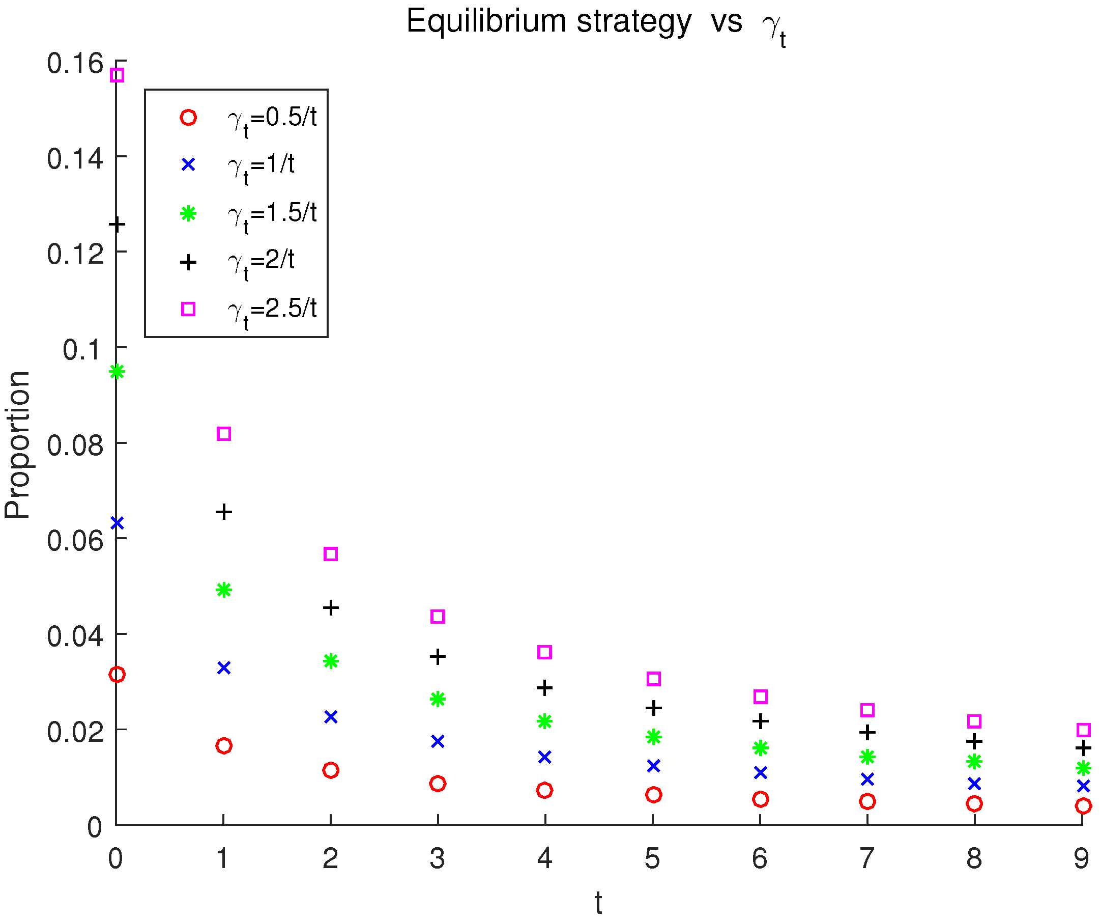
(1) Effect of the risk aversion coefficient on the equilibrium strategy
Let
and the risk aversion coefficient is
. The equilibrium strategy corresponding to the increasing risk aversion coefficient
is demonstrated in
Figure 1. We can see from
Figure 1 that the investment in the risky asset decreases over time for each
. Moreover, as
increases, the investment proportion in the risky asset increases at each period. The reason behind this is that the larger the value of
is, the lower the degree of the investor’s risk aversion is at time
t, which then generates larger investment in the risky asset. This result is consistent with the results in Cui et al. [
16], Wang and Chen [
14] and also matches the reality that the investor will shift his investment from the risky asset to a safe or less risky asset with the coming of the terminal time.
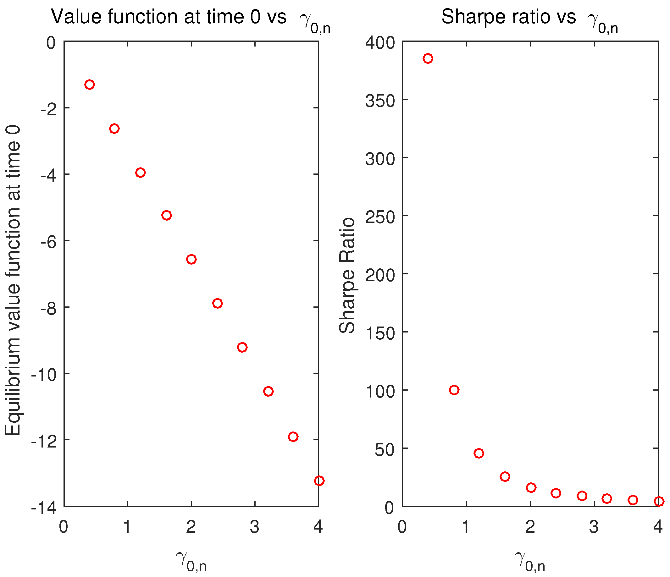
(2) Effect of the risk aversion coefficient on the equilibrium value function
The left-hand side of
Figure 2 shows that the equilibrium value function at the initial time decreases as the risk aversion coefficient at the initial time increases. Wu and Chen [
30] show a similar result when the volatility of the risk aversion changes and point out that the volatility of the risk aversion, as a component of risk, plays an important role in the equilibrium value function. As our risk aversion parameter is state-dependent, even though the risk aversion coefficient at the initial time increases with the same volatility, the volatility of our risk aversion parameter is still changing.
(3) Effect of the risk aversion coefficient on the Sharpe ratio
Define
as the Sharpe ratio of the terminal wealth achieved by the equilibrium strategy. We choose this Sharpe ratio as a performance index to show the global investment performance of the equilibrium strategy. Let the risk aversion coefficient
fluctuate as (31) shows, the relationship between the Sharpe ratio and the risk aversion coefficient at the initial time is depicted in the right-hand side of
Figure 2. We find that increasing the risk aversion coefficient at the initial time gives rise to a decrease in the Sharpe ratio of the terminal wealth. As
increases, the risk aversion of the investor decreases and the investment amount in the risky asset increases, which generates larger mean and variance of the terminal wealth. This observation shows that the variance of the terminal wealth increases faster than that of the expected value of the terminal wealth, which indicates that the incorporation of the successive contribution brings extra risk for the investor.
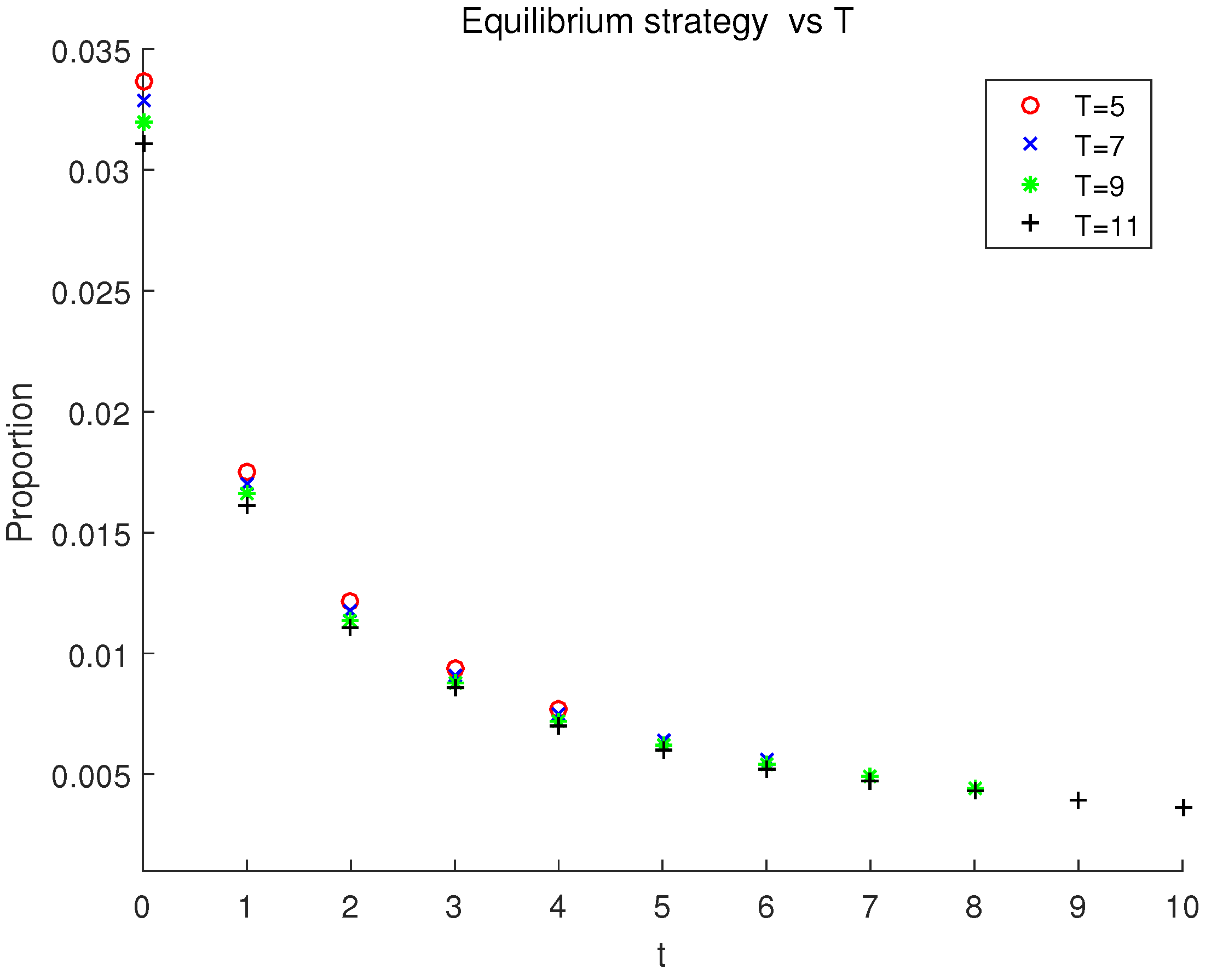
To obtain a more comprehensive understanding, we further analyze the influence of the investment time horizon and the contribution rate on the equilibrium strategy. In the following experiments, and remain the initial values, the risk aversion coefficient is
Let
and the investment horizon
T increase from 5 to 11 with step size 2, the equilibrium strategies under different
Ts are demonstrated in
Figure 3. We can draw some conclusions from this figure: (1) The allocation in the risky asset decreases during the whole investment horizon for each
T. (2) The shorter the investment horizon
T is, the larger the proportion holds in the risky asset at each period. This is easy to understand since the investor would have less confidence to control the investment uncertainty in the future when the investment horizon becomes longer, which results in smaller investment amount in the risky asset. (3) The longer the investment horizon
T is, the smaller the proportion holds in the risky asset at the terminal time, which is quite different with Wu and Chen [
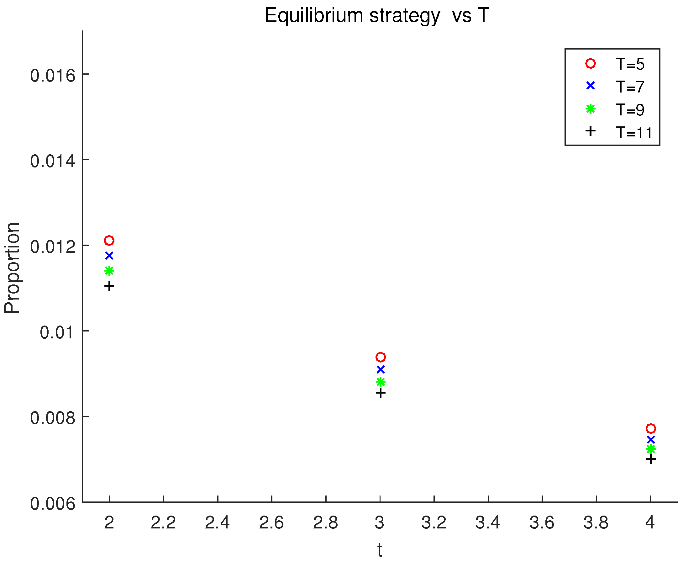
30]. Although we contribute to the pension account at each period, our accumulated wealth is basically increasing throughout the investment period. Noting that the risk aversion coefficient decreases with respect to time. The third conclusion implies that, when the investment horizon becomes longer, the decrease of the risk aversion coefficient is more pronounced than the increase of the accumulated wealth, which leads to a decrease in the risk aversion function, that is, the investor becomes more risk averse. All in all, the investment proportion in the risky asset will be smaller as the investment horizon
T becomes longer. To get a closer look, an amplified version for
is given in
Figure 4.
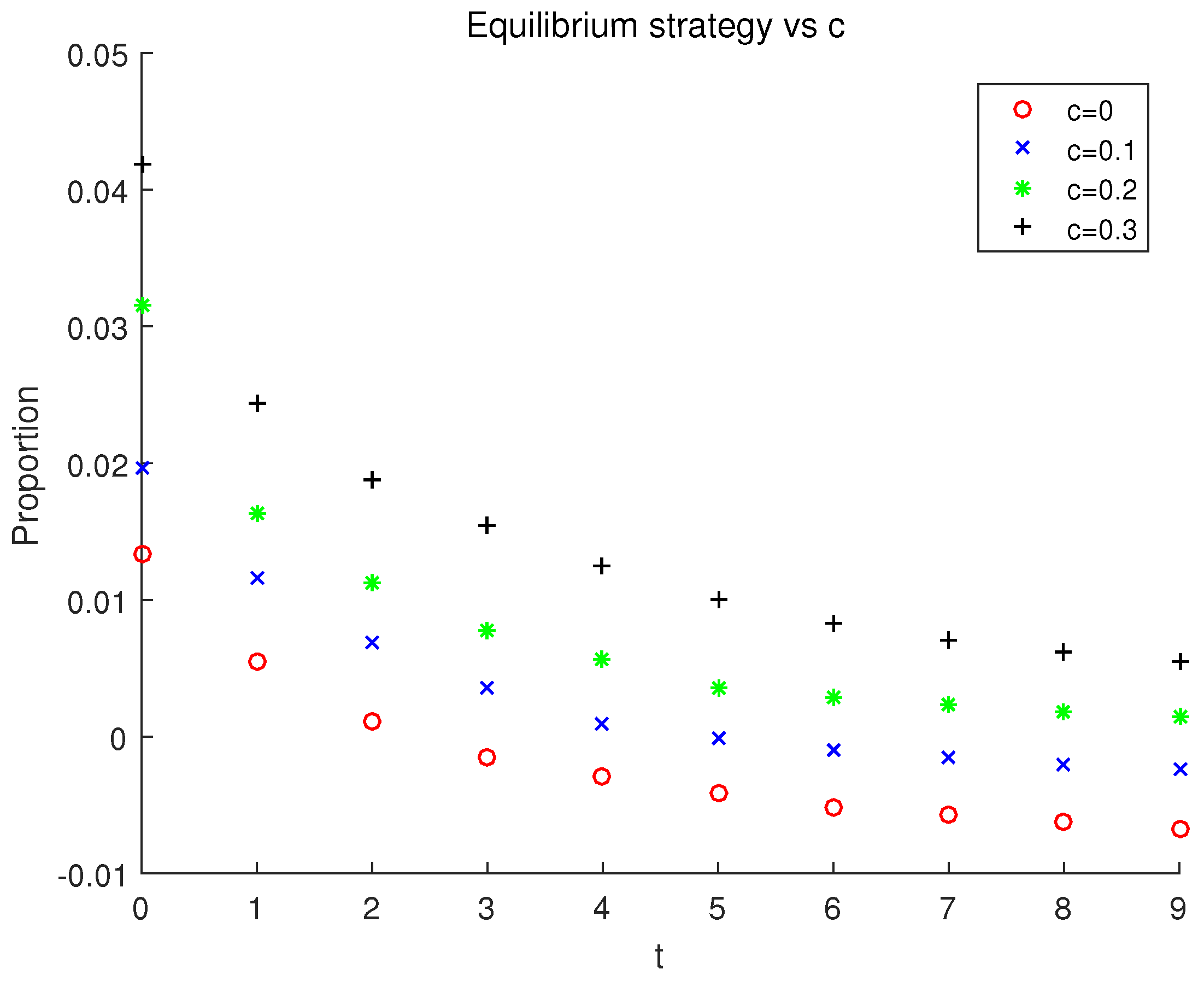
Finally, we examine the effect of the contribution rate
c on the equilibrium strategy. Let
and the contribution rate
c increase from 0 to 0.3 with step size 0.1. Our natural intuition is that a larger investment comes with a higher contribution rate, as it directly leads to a higher accumulated wealth for the pension fund. Apparently, the result shown in
Figure 5 validates our intuitive idea. We observe from
Figure 5 that: (1) The investment proportion in the risky asset increases at each period as
c increases. (2) The investment in the risky asset decreases over time under each
c. (3) When
, the investment in the risky asset is the lowest, and the speed of the decrease is the slowest compared with the other three cases.
Remark 12. The above numerical results are consistent with the results in Wang and Chen [14] in essential. In the above numerical tests, we use a risk aversion coefficient linked to the investor’s risk aversion attitude, (i.e., ), while in Wang and Chen [14], we simply assume that the risk aversion coefficient is a constant. It is clear that the choice of the risk aversion coefficient in this paper is more reasonable and the results are more realistic. It seems that the positiveness of the wealth process have little impact. However, for the numerical tests in Wang and Chen [14], we actually need to adjust the related parameters many times to ensure that the wealth level is positive. In this paper, this parameter adjustment is not needed. All the above numerical results and analyses further illustrate the theoretical results we have drawn and help us comprehend this paper easily.


