A Time-Non-Homogeneous Double-Ended Queue with Failures and Repairs and Its Continuous Approximation

 ,
,  , and
, and 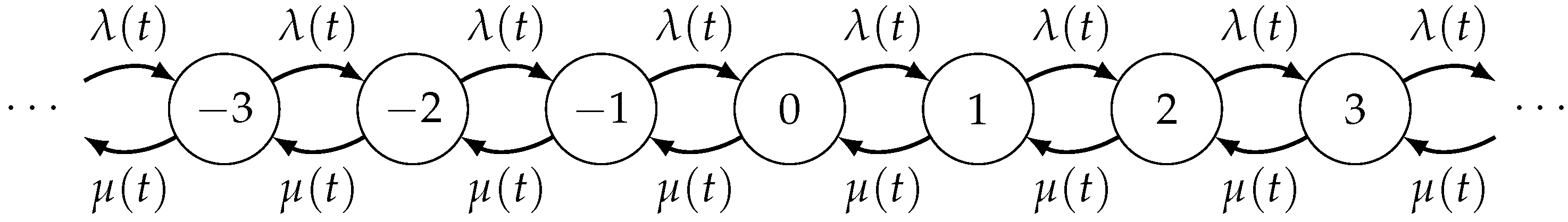
Abstract
:1. Introduction
- Queueing systems subject to disasters are appropriate to model more realistic situations in which the number of customers is subject to an abrupt decrease by the effect of catastrophes occurring randomly in time and due to external causes. The literature on the area of stochastic systems evolving in the presence of catastrophes is very broad. We restrict ourselves to mentioning the papers by Economou and Fakinos [15,16], Kyriakidis and Dimitrakos [17], Krishna Kumar et al. [18], Di Crescenzo et al. [19], Zeifman and Korotysheva [20], Zeifman et al. [21] and Giorno et al. [22]. The analysis of some time-dependent queueing models with catastrophes has been performed in Di Crescenzo et al. [23] and, more recently, in Giorno et al. [24], with special attention to the and queues.
- We include a repair mechanism in the queueing system under investigation, since it is essential to model instances when the (random) repair times are not negligible. We remark that the interest in this feature is increasing in the recent literature on queueing theory (see, for instance, Dimou and Economou [25]).
- Heavy-traffic approximations are very often proposed in order to describe the queueing systems under proper limit conditions of the parameters involved. This allows one to come to more manageable formulas for the description of the queue content. Typically, a customary rescaling procedure allows one to approximate the queue length process by a diffusion process, as indicated in Giorno et al. [26]. Examples of diffusion models arising from heavy-traffic approximations of double-ended queues and of similar matching systems can be found in Liu et al. [27] and Büke and Chen [28], respectively. In the case of queueing systems subject to catastrophes, a customary approach leads to jump-diffusion approximating processes (see, for instance, Di Crescenzo et al. [29] and Dharmaraja et al. [30]).
Plan of the Paper
2. The Underlying Non-Homogeneous Double-Ended Queue
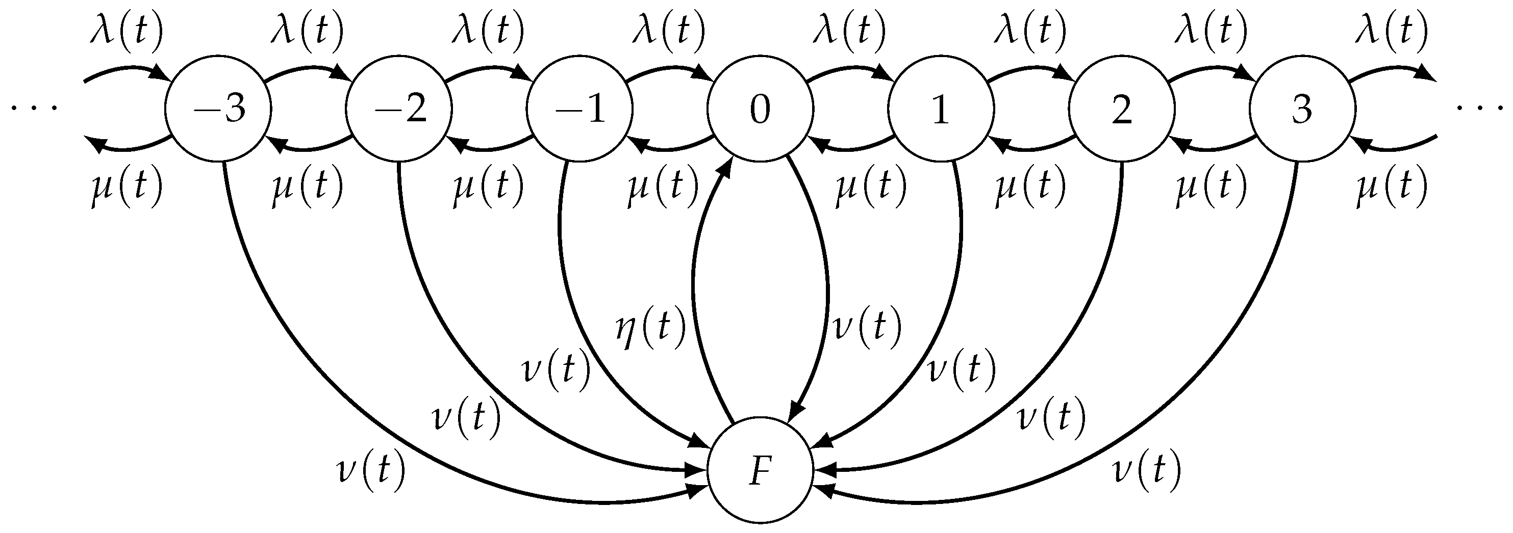
3. The Queueing System with Catastrophes and Repairs
Transient Probabilities
- -
- starting from zero at time , at least a catastrophe and the subsequent repair occur before t; let be the instant at which the last repair occurs, so that a transition entering in the zero state occurs at time with intensity ;
- -
- no catastrophe occurs in the interval ; then the system, starting from the zero state at time , reaches the state n at time t.
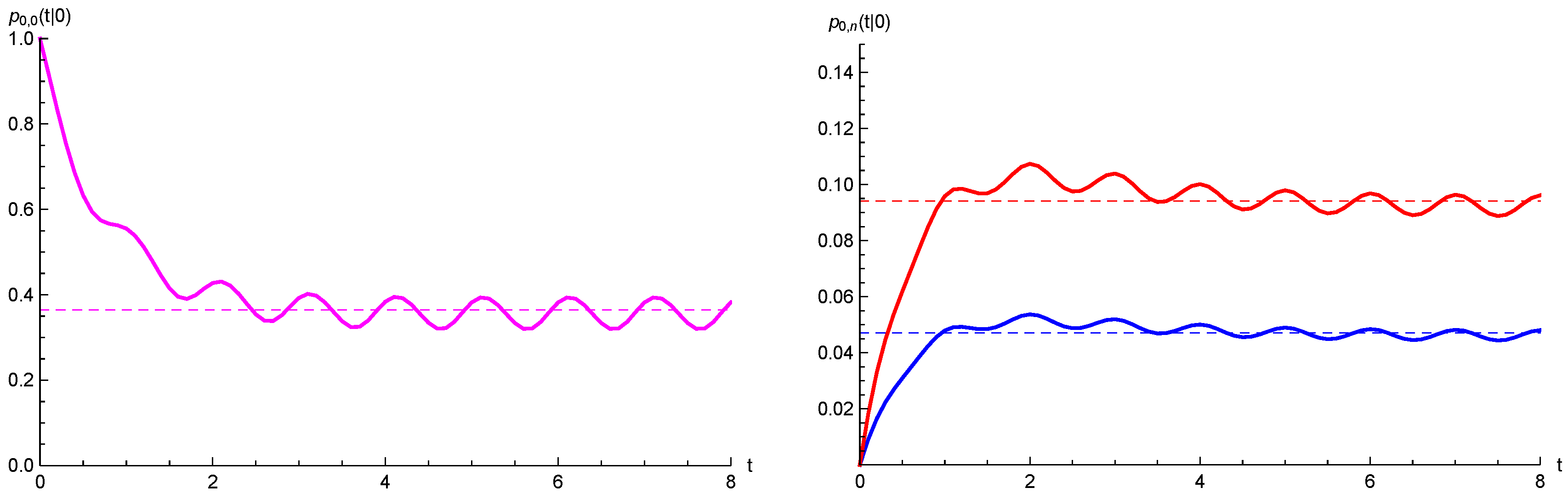
4. Asymptotic Probabilities
- (i)
- the intensity functions and admit finite positive limits as ,
- (ii)
- the intensity functions and are constant, whereas the rates and are periodic functions with common period Q.
4.1. Asymptotically-Constant Intensity Functions
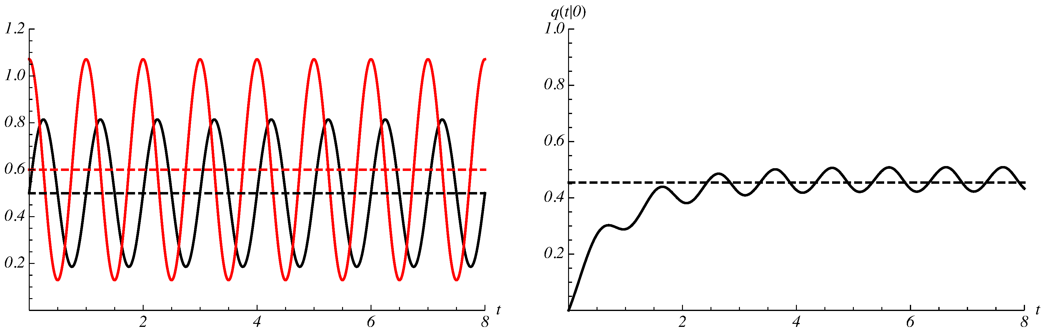
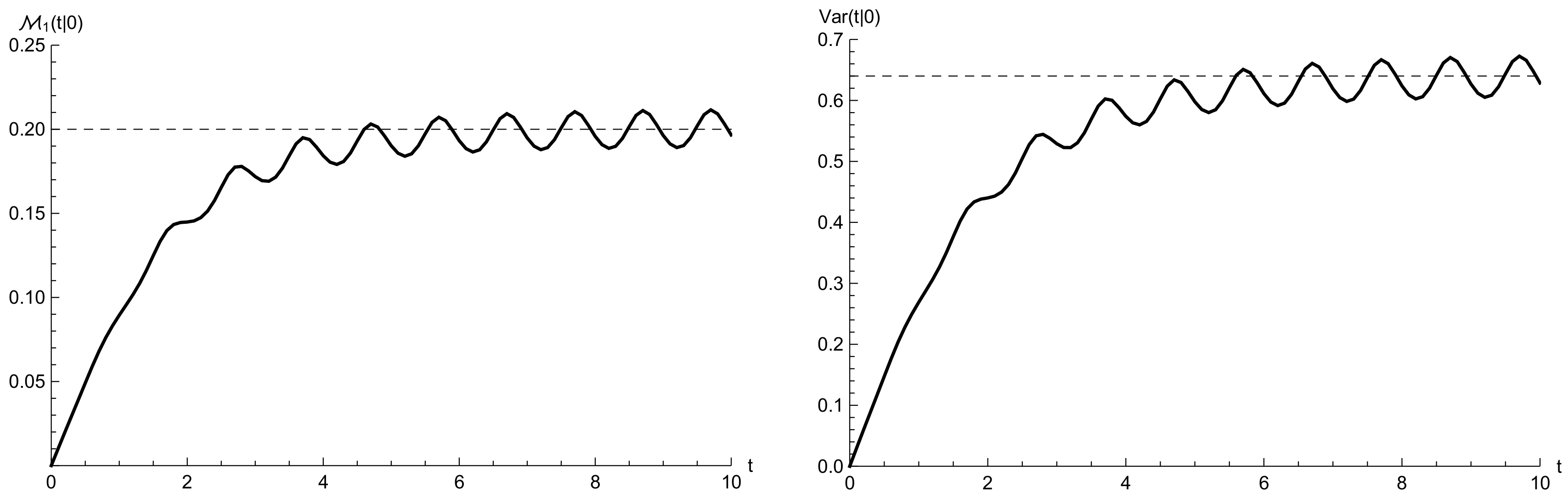
4.2. Periodic Catastrophe and Repair Intensity Functions
5. Diffusion Approximation of the Double-Ended Queueing System
Goodness of the Approximating Procedure
6. Diffusion Approximation of the Double-Ended Queueing System with Catastrophes and Repairs
6.1. Transient Distribution
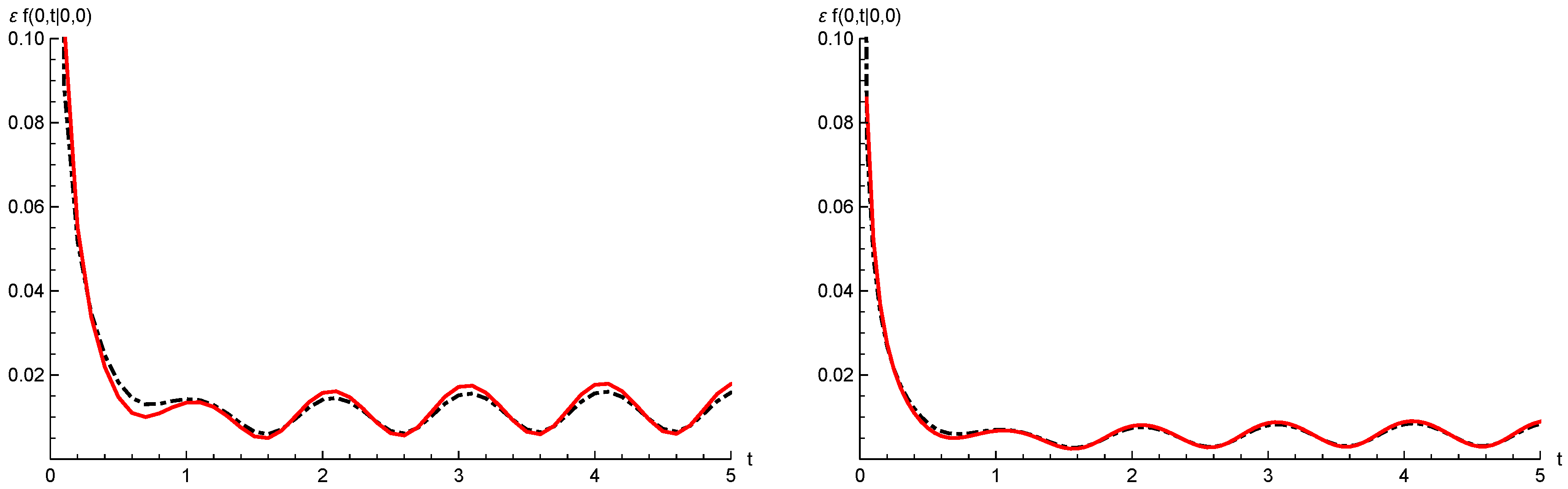
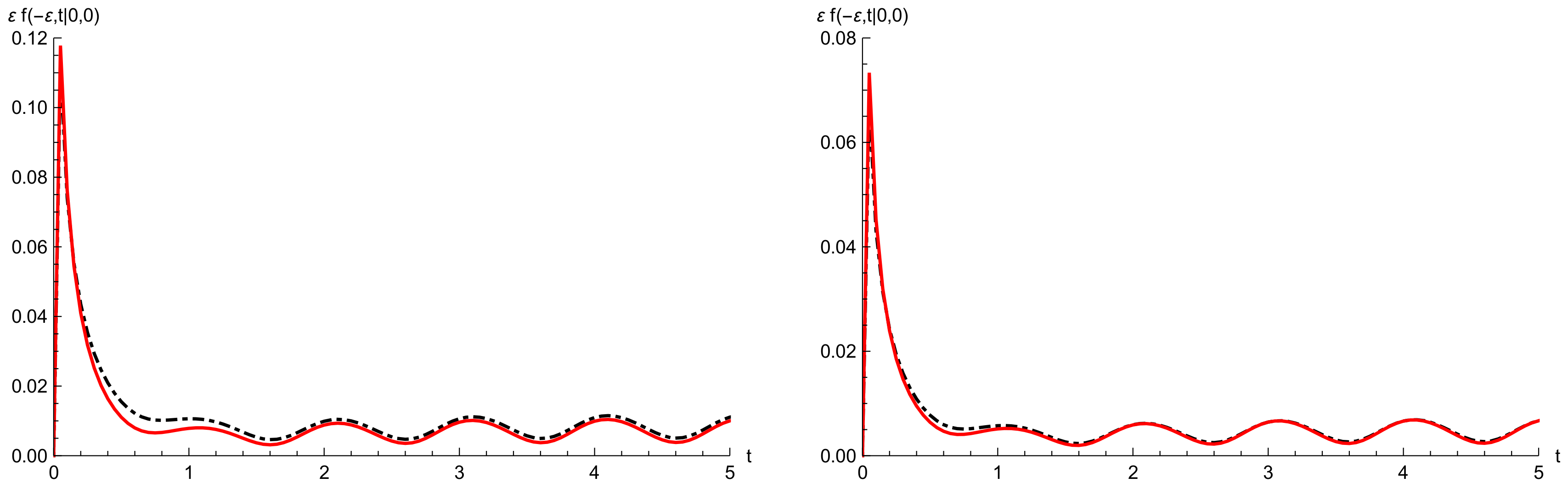
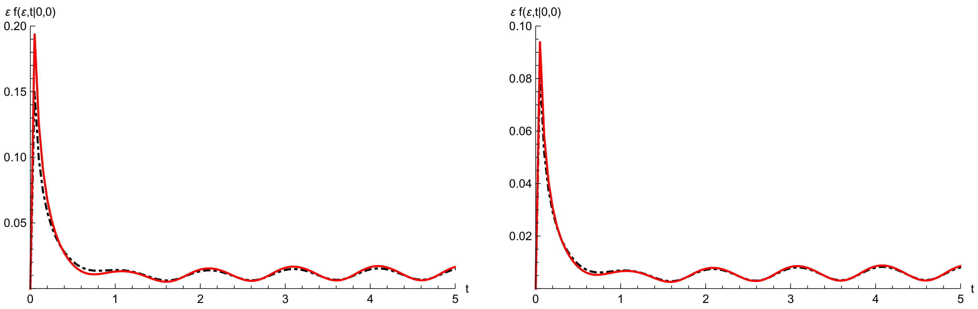
6.2. Goodness of the Approximating Procedure
7. Asymptotic Distributions
- (i)
- the functions , , , and admit finite positive limits as ,
- (ii)
- the functions , and are constant, and the rates and are periodic functions with common period Q.
7.1. Asymptotically-Constant Intensity Functions
7.2. Periodic Intensity Functions
8. Conclusions
Author Contributions
Acknowledgments
Conflicts of Interest
References
- Kashyap, B.R.K. A double-ended queueing system with limited waiting space. Proc. Natl. Inst. Sci. India A 1965, 31, 559–570. [Google Scholar] [CrossRef]
- Kashyap, B.R.K. The double-ended queue with bulk service and limited waiting space. Oper. Res. 1966, 14, 822–834. [Google Scholar] [CrossRef]
- Sharma, O.P.; Nair, N.S.K. Transient behaviour of a double ended Markovian queue. Stoch. Anal. Appl. 1991, 9, 71–83. [Google Scholar] [CrossRef]
- Tarabia, A.M.K. On the transient behaviour of a double ended Markovian queue. J. Combin. Inf. Syst. Sci. 2001, 26, 125–134. [Google Scholar]
- Conolly, B.W.; Parthasarathy, P.R.; Selvaraju, N. Doubled-ended queues with impatience. Comput. Oper. Res. 2002, 29, 2053–2072. [Google Scholar] [CrossRef]
- Elalouf, A.; Perlman, Y.; Yechiali, U. A double-ended queueing model for dynamic allocation of live organs based on a best-fit criterion. Appl. Math. Model. 2018, in press. [Google Scholar] [CrossRef]
- Takahashi, M.; Ōsawa, H.; Fujisawa, T. On a synchronization queue with two finite buffers. Queueing Syst. 2000, 36, 107–123. [Google Scholar] [CrossRef]
- Di Crescenzo, A.; Giorno, V.; Nobile, A.G. Constructing transient birth-death processes by means of suitable transformations. Appl. Math. Comput. 2016, 281, 152–171. [Google Scholar] [CrossRef]
- Di Crescenzo, A.; Giorno, V.; Nobile, A.G. Analysis of reflected diffusions via an exponential time-based transformation. J. Stat. Phys. 2016, 163, 1425–1453. [Google Scholar] [CrossRef]
- Di Crescenzo, A.; Giorno, V.; Krishna Kumar, B.; Nobile, A.G. A double-ended queue with catastrophes and repairs, and a jump-diffusion approximation. Methodol. Comput. Appl. Probab. 2012, 14, 937–954. [Google Scholar] [CrossRef]
- Altiok, T. On the phase-type approximations of general distributions. IIE Trans. 1985, 17, 110–116. [Google Scholar] [CrossRef]
- Altiok, T. Queueing modeling of a single processor with failures. Perform. Eval. 1989, 9, 93–102. [Google Scholar] [CrossRef]
- Altiok, T. Performance Analysis of Manufacturing Systems. Springer Series in Operations Research; Springer: New York, NY, USA, 1997. [Google Scholar]
- Dallery, Y. On modeling failure and repair times in stochastic models of manufacturing systems using generalized exponential distributions. Queueing Syst. 1994, 15, 199–209. [Google Scholar] [CrossRef]
- Economou, A.; Fakinos, D. A continuous-time Markov chain under the influence of a regulating point process and applications in stochastic models with catastrophes. Eur. J. Oper. Res. 2003, 149, 625–640. [Google Scholar] [CrossRef]
- Economou, A.; Fakinos, D. Alternative approaches for the transient analysis of Markov chains with catastrophes. J. Stat. Theory Pract. 2008, 2, 183–197. [Google Scholar] [CrossRef]
- Kyriakidis, E.; Dimitrakos, T. Computation of the optimal policy for the control of a compound immigration process through total catastrophes. Methodol. Comput. Appl. Probab. 2005, 7, 97–118. [Google Scholar] [CrossRef]
- Krishna Kumar, B.; Vijayakumar, A.; Sophia, S. Transient analysis for state-dependent queues with catastrophes. Stoch. Anal. Appl. 2008, 26, 1201–1217. [Google Scholar] [CrossRef]
- Di Crescenzo, A.; Giorno, V.; Nobile, A.G.; Ricciardi, L.M. A note on birth-death processes with catastrophes. Stat. Probab. Lett. 2008, 78, 2248–2257. [Google Scholar] [CrossRef]
- Zeifman, A.; Korotysheva, A. Perturbation bounds for Mt/Mt/N queue with catastrophes. Stoch. Models 2012, 28, 49–62. [Google Scholar] [CrossRef]
- Zeifman, A.; Satin, Y.; Panfilova, T. Limiting characteristics for finite birth-death-catastrophe processes. Math. Biosci. 2013, 245, 96–102. [Google Scholar] [CrossRef] [PubMed]
- Giorno, V.; Nobile, A.G.; Pirozzi, E. A state-dependent queueing system with asymptotic logarithmic distribution. J. Math. Anal. Appl. 2018, 458, 949–966. [Google Scholar] [CrossRef]
- Di Crescenzo, A.; Giorno, V.; Nobile, A.G.; Ricciardi, L.M. On time non-homogeneous stochastic processes with catastrophes. In Cybernetics and Systems 2010, Proceedings of the Austrian Society for Cybernetics Studies (EMCSR 2010), Vienna, Austria, 6–9 April 2010; Trappl, R., Ed.; Austrian Society for Cybernetic Studies: Vienna, Austria, 2010; pp. 169–174. [Google Scholar]
- Giorno, V.; Nobile, A.G.; Spina, S. On some time non-homogeneous queueing systems with catastrophes. Appl. Math. Comput. 2014, 245, 220–234. [Google Scholar] [CrossRef]
- Dimou, S.; Economou, A. The single server queue with catastrophes and geometric reneging. Methodol. Comput. Appl. Probab. 2013, 15, 595–621. [Google Scholar] [CrossRef]
- Giorno, V.; Nobile, A.G.; Ricciardi, L.M. On some time-non-homogeneous diffusion approximations to queueing systems. Adv. Appl. Probab. 1987, 19, 974–994. [Google Scholar] [CrossRef]
- Liu, X.; Gong, Q.; Kulkarni, V.G. Diffusion models for double-ended queues with renewal arrival processes. Stoch. Syst. 2015, 5, 1–61. [Google Scholar] [CrossRef]
- Büke, B.; Chen, H. Fluid and diffusion approximations of probabilistic matching systems. Queueing Syst. 2017, 86, 1–33. [Google Scholar] [CrossRef]
- Di Crescenzo, A.; Giorno, V.; Nobile, A.G.; Ricciardi, L.M. On the M/M/1 queue with catastrophes and its continuous approximation. Queueing Syst. 2003, 43, 329–347. [Google Scholar] [CrossRef]
- Dharmaraja, S.; Di Crescenzo, A.; Giorno, V.; Nobile, A.G. A continuous-time Ehrenfest model with catastrophes and its jump-diffusion approximation. J. Stat. Phys. 2015, 161, 326–345. [Google Scholar] [CrossRef]
- Abramowitz, M.; Stegun, I. Handbook of Mathematical Functions with Formulas, Graphs and Mathematical Tables; Dover Publications, Inc.: New York, NY, USA, 1972. [Google Scholar]
- Irwin, J.O. The frequency-distribution of the difference between two independent variates following the same Poisson distribution. J. R. Stat. Soc. 1937, 100, 415–416. [Google Scholar] [CrossRef]
- Skellam, J.G. The frequency-distribution of the difference between two Poisson variates belonging to different populations distribution. J. R. Stat. Soc. 1946, 109, 296. [Google Scholar] [CrossRef]
- Buonocore, A.; Di Crescenzo, A.; Giorno, V.; Nobile, A.G.; Ricciardi, L.M. A Markov chain-based model for actomyosin dynamics. Sci. Math. Jpn. 2009, 70, 159–174. [Google Scholar]


© 2018 by the authors. Licensee MDPI, Basel, Switzerland. This article is an open access article distributed under the terms and conditions of the Creative Commons Attribution (CC BY) license (http://creativecommons.org/licenses/by/4.0/).
Share and Cite
Di Crescenzo, A.; Giorno, V.; Krishna Kumar, B.; Nobile, A.G. A Time-Non-Homogeneous Double-Ended Queue with Failures and Repairs and Its Continuous Approximation. Mathematics 2018, 6, 81. https://doi.org/10.3390/math6050081
Di Crescenzo A, Giorno V, Krishna Kumar B, Nobile AG. A Time-Non-Homogeneous Double-Ended Queue with Failures and Repairs and Its Continuous Approximation. Mathematics. 2018; 6(5):81. https://doi.org/10.3390/math6050081
Chicago/Turabian StyleDi Crescenzo, Antonio, Virginia Giorno, Balasubramanian Krishna Kumar, and Amelia G. Nobile. 2018. "A Time-Non-Homogeneous Double-Ended Queue with Failures and Repairs and Its Continuous Approximation" Mathematics 6, no. 5: 81. https://doi.org/10.3390/math6050081