Article

An Estimate of the Root Mean Square Error Incurred When Approximating an fL2(ℝ) by a Partial Sum of Its Hermite Series

Department of Mathematics and Statistics, Brock University, St. Catharines, L2S 3A1, ON, Canada
*
Author to whom correspondence should be addressed.
Mathematics 2018, 6(4), 64; https://doi.org/10.3390/math6040064
Submission received: 29 January 2018 / Revised: 17 March 2018 / Accepted: 17 April 2018 / Published: 23 April 2018
(This article belongs to the Special Issue Applied Mathematics and Mechanics 2017)

Abstract

:
Let f be a band-limited function in L 2 ( R ) . Fix T > 0 , and suppose f exists and is integrable on [ T , T ] . This paper gives a concrete estimate of the error incurred when approximating f in the root mean square by a partial sum of its Hermite series. Specifically, we show, that for K = 2 n , n Z + , 1 2 T T T [ f ( t ) ( S K f ) ( t ) ] 2 d t 1 / 2 1 + 1 K 1 2 T | t | > T f ( t ) 2 d t 1 / 2 + 1 2 T | ω | > N | f ^ ( ω ) | 2 d ω 1 / 2 + 1 K 1 2 T | t | T f N ( t ) 2 d t 1 / 2 + 1 π 1 + 1 2 K S a ( K , T ) , in which S K f is the K-th partial sum of the Hermite series of f , f ^ is the Fourier transform of f, N = 2 K + 1 + 2 K + 3 2 and f N = ( f ^ χ ( N , N ) ) ( t ) = 1 π sin ( N ( t s ) ) t s f ( s ) d s . An explicit upper bound is obtained for S a ( K , T ) .

1. Introduction

The aim of this paper is to give a concrete estimate of the error incurred when approximating a function f in the root mean square by a partial sum, S K f , of its Hermite series. The source of the estimate, the fact that the estimate is numerical rather than just an order of magnitude and the centrality of the so-called Dirichlet operator to the partial sum are all discussed following the statement below of our principal result.
Hermite series, often under the name Gram–Charlier series of Type A, are used to approximate probability density functions, which are key to statistical inference [1] in such fields as: visual image processing in engineering [2], reliability ([3], Chapter 3), econometrics [4], quantile regression [5], big data in nonparametric statistics ([6], Chapters 1 and 2) and machine learning in artificial intelligence ([7], Chapter 5). In Section 5 of this paper, we apply our estimates to the Hermite series approximation of a trimodal density function from [8] (pp. 176–178); see also [9].
Again, as observed in [10] and the references therein, Hermite functions are the exact unperturbed eigenfunctions or the limiting asymptotic eigenfunctions (Mathieu functions, prolate spheroidal wave functions) for many problems of physical interest, Thus, Hermite series arise, for example, in the study of the harmonic oscillator in quantum mechanics and of equatorial waves in dynamic meteorology and oceanography.
We recall that the k-th Hermite function, h k , is given at t R by:
h k ( t ) = ( 1 ) k γ k e t 2 2 d k e t 2 d t k , k = 0 , 1 , ,
where γ k = π 1 / 4 2 k / 2 ( k ! ) 1 / 2 . Given f L 2 ( R ) , its Hermite series is:
k = 0 c k h k ,
in which:
c k = R f ( t ) h k ( t ) d t , k = 0 , 1 , 2 , .
Our principal result is:
Theorem 1.
Consider a band-limited function f L 2 ( R ) . Fix T > 0 , and suppose f exists and is integrable on I T = [ T , T ] .
Then, with K = 2 n , n Z + , S K f the K-th partial sum of the Hermite series of f and:
N = 2 K + 1 + 2 K + 3 2 ,
one has:
1 2 T T T [ f ( t ) ( S K f ) ( t ) ] 2 d t 1 / 2 1 + 1 K 1 2 T | t | > T f ( t ) 2 d t 1 / 2 + 1 2 T | ω | > N | f ^ ( ω ) | 2 d ω 1 / 2 + 1 K 1 2 T | t | T f N ( t ) 2 d t 1 / 2 + 1 π 1 + 1 2 K S a ( K , T ) ,
in which f N = ( f ^ χ ( N , N ) ) .
We work with an expression for S 2 n f , n = 0 , 1 , 2 , , due to G. Sansone [11], the which expression is a refinement of the one employed by J.V. Uspensky in [12] to prove his classical convergence theorems for Hermite series (the treatment of S 2 n + 1 f , n = 0 , 1 , 2 , , is similar).
As seen from Formulas (2) and (5) below, the core of S 2 n f is the Dirichlet operator:
( F N f ) ( t ) = 1 π T T sin N ( t s ) t s f ( s ) d s ,
in which N = 4 n + 1 + 4 n + 3 2 and t [ T , T ] , T > 0 . We have cut the time content of f outside [ T , T ] and the frequency content greater than N, so that our assertion about the Dirichlet operator requires f to be almost time-limited in [ T , T ] and the frequency content almost band-limited in [ N , N ] . Moreover, the estimates we give in Section 3 of the terms other than:
1 2 T | α | > t f ( α ) 2 d α 1 / 2 + 1 2 T | ω | > N | f ^ ( ω ) | 2 d ω 1 / 2
in the estimate of 1 2 T T T | f ( x ) ( S K f ) ( x ) | 2 d x 1 / 2 in Formula (5) below in Section 4 quantify how far f S n f , or rather f F N f , is from zero in the root mean square on [ T , T ] . The application of these estimates in our example is straightforward (though somewhat tedious) given the material in Appendix A. We emphasize that the estimates are in numbers and not in orders of magnitude.
A key fact, used repeatedly in the derivation at our estimates, is that the Hilbert transform, H, given, for suitable f at almost all x R by:
( H f ) ( x ) = 1 π ( P ) R f ( y ) x y d y = 1 π lim ε 0 + | x y | > ε f ( y ) x y d y ,
is a unitary operator on L 2 ( R ) . Also important will be certain identities of Bedrosian, valid for band-limited functions f L 2 ( R ) , namely,
H ( f sin ( a · ) ) ( t ) = f ( t ) cos a t
and:
H ( f cos ( b · ) ) ( t ) = f ( t ) sin b t , t R ,
for fixed a , b R . See [13].
The error involved in approximating f by F N f is established in Lemma 1 in the next section. The Sansone estimates are intensively studied in Section 3. These enable the proof of Theorem 1 in the following section, where S a ( n , T ) is defined. An explicit estimate of S a ( n , T ) is described in Appendix A.
The estimate of the root mean square error in (1) is both more specific and more easily calculated than the one in the paper [9] of the first two authors and M. Brannan. In the final section, we revisit the trimodal distribution studied in that paper.

2. Approximation Using the Dirichlet Operator

In this section, we prove:
Lemma 1.
Given f L 2 ( R ) , N , T R + , and f T = f χ ( T , T ) , set:
( F N f T ) ( t ) = 1 π T T sin ( N ( t s ) ) t s f ( s ) d s , t I T = [ T , T ] .
Then,
1 2 T T T | f ( t ) ( F N f T ) ( t ) | 2 d t 1 / 2 d t 1 2 T | t | > T | f ( t ) | 2 d t 1 / 2 + 1 2 T | ω | > N | f ^ ( ω ) | 2 d ω 1 / 2
Note, we define the Fourier transform, f ^ , of f by f ^ ( ω ) = 1 2 π R f ( t ) e i ω t d t , ω R .
Proof. 
Using the standard notation s i n c t = sin t t , we have:
F N f T = 2 π N ( s i n c t ) f T , t R .
Here, the convolution, g h , of g and h in L 2 ( R ) is here defined by ( g h ) ( t ) = 1 2 π g ( t s ) h ( s ) d s , t R . One has ( g h ) ( ω ) = g ( ω ) h ( ω ) , ω R . See [14].
whence:
F N f T ^ = χ ( N , N ) f ^ T .
Thus,
T T | f ( t ) ( F N f T ) ( t ) | 2 d t 1 / 2 R | f ( t ) ( F N f T ) ( t ) | 2 d t 1 / 2 = R + | f ^ ( ω ) F N f T ^ ( ω ) | 2 d ω 1 / 2 = R | f T ^ ( ω ) χ ( N , N ) f ^ ( ω ) T | 2 d ω 1 / 2 = | ω | > N | f ^ T ( ω ) | 2 d ω 1 / 2 = | ω | > N 1 2 π T T f ( y ) e i ω y d y 2 d ω 1 / 2 | ω | > N 1 2 π R χ T ( y ) f ( y ) e i ω y d y 2 d ξ 1 / 2 = | ω | > N ( χ T f ^ ( ω ) 2 d ω 1 / 2 | ω | > N f ^ ( ω ) 2 d ω 1 / 2 + | ω | > N ( χ | t | > T f ) ^ ( ω ) 2 d ω 1 / 2 | ω | > N f ^ ( ω ) 2 d ω 1 / 2 + R ( χ | t | > T f ) ^ ( ω ) 2 d ω 1 / 2 | ω | > N f ^ ( ω ) 2 d ω 1 / 2 + | t | > T f ( t ) 2 d t 1 / 2 .

3. The Sansone Estimates

To begin, we describe Sansone’s analysis of the usual expression for ( K f T ) ( t ) = k = 0 K c k h k ( t ) , when K is even, say K = 2 n . For ease of reference to [12], we work with the variables x and α, rather than t and s.
Now, according to [11] (p. 372, (4) and (5)),
( S 2 n f ) ( x ) = 2 n + 1 2 T T k 2 n ( x , α ) f ( α ) d α ,
where:
k 2 n ( x , α ) = h 2 n + 1 ( x ) h 2 n ( α ) h 2 n + 1 ( α ) h 2 n ( x ) α x
and f T = f T χ I . Further, by (7) and (8) on p. 373 and the first two estimates on p. 374, together with (15.1) and (15.2) on p. 362, one has:
2 k + 1 2 k 2 n ( x , α ) ( x α ) = C ( n ) [ A ( x ) B ( α ) A ( α ) B ( x ) ] ,
in which:
C ( n ) = 1 π 1 + ε 12 n , | ε | < 3 ,
A ( y ) = sin ( 4 n + 3 y ) y 3 6 cos ( 4 n + 3 y ) 4 n + 3 + T ( 2 n + 1 , y ) h 2 n + 1 ( 0 ) 4 n + 3
and:
B ( y ) = cos ( 4 n + 1 y ) y 3 6 sin ( 4 n + 1 y ) 4 n + 1 + T ( 2 n , α ) h 2 n ( 0 ) 4 n + 1 .
The functions T ( 2 n , y ) and T ( 2 n + 1 , y ) are defined through the equations:
h 2 n ( x ) = h 2 n ( 0 ) cos ( 4 n + 1 x ) + h 2 n ( 0 ) 4 n + 1 y 3 6 sin ( 4 n + 1 y ) + T ( 2 n , y ) 4 n + 1
and:
h 2 n + 1 ( y ) = h 2 n + 1 ( 0 ) sin ( 4 n + 3 y ) 4 n + 3 h 2 n + 1 ( 0 ) 4 n + 3 y 3 6 cos ( 4 n + 3 y ) + T ( 2 n + 1 , y ) 4 n + 3 .
Here,
| a n | = 1 | h 2 n + 1 ( 0 ) | 1 4 n + 3 < 4 π 1 / 2 3 2 4 1 n 3 / 4 ,
| b n | = 1 | h 2 n ( 0 ) | 1 4 n + 1 < π 1 / 2 4 3 2 4 1 n 3 / 4 ,
| T ( 2 n + 1 , y ) | < y 2 π 1 / 2 n 1 / 4 y 4 18 + 1 + 4 187 y 17 / 2 4 n + 1
and:
| T ( 2 n , y ) | < y 2 π 1 / 2 n 1 / 4 y 4 18 + 1 + 4 187 y 17 / 2 4 n + 3 .
Expanding the products in (3) yields:
2 n + 1 2 k 2 n ( x , α ) ( x α ) = 1 π 1 + ε 6 K sin ( N ( x α ) ) + k = 1 5 M k ( n ) ( x , α ) , | ε | < 3 ,
where, firstly,
M 1 ( n ) ( x , α ) = cos ( N ( x + α ) ) sin ( ( x α ) / 2 N ) 2 sin 2 ( ( x + α ) / 4 N ) sin ( N ( x α ) ) ,
as shown on p. 375 of [11]. Again, on p. 376, we find:
4 n + 1 M 2 ( n ) ( x , α ) = x 3 6 sin ( 4 n + 1 x ) sin ( 4 n + 3 α ) + α 3 6 sin ( 4 n + 1 α ) sin ( 4 n + 3 x ) = α 3 x 3 6 sin ( 4 n + 1 x ) sin ( 4 n + 3 α ) + α 3 6 sin ( ( x α ) / 2 N ) sin ( N ( x + α ) ) sin ( ( x + α ) / 2 N ) sin ( N ( x α ) ) .
An argument similar to the one for 4 n + 1 M 2 ( n ) ( x , α ) gives:
4 n + 3 M 3 ( n ) ( x , α ) = α 3 6 cos ( 4 n + 1 x ) cos ( 4 n + 3 α ) x 3 6 cos ( 4 n + 1 α ) cos ( 4 n + 3 x ) = α 3 x 3 6 cos ( 4 n + 1 x ) cos ( 4 n + 3 x ) x 3 6 cos ( 4 n + 1 α ) cos ( 4 n + 3 x ) cos ( 4 n + 1 x ) cos ( 4 n + 3 α ) = α 3 x 3 6 cos ( 4 n + 1 x ) cos ( 4 n + 3 α ) x 3 6 [ sin ( N ( x + α ) ) sin ( ( x α ) / 2 N ) + sin ( ( x + α ) / 2 N ) sin ( N ( x α ) ) ] .
Next,
( 4 n + 1 ) ( 4 n + 3 ) M 4 ( n ) ( x , α ) = α 3 x 3 36 [ cos ( 4 n + 3 x ) sin ( 4 n + 1 α ) + cos ( 4 n + 3 α ) sin ( 4 n + 1 x ) ] = α 3 x 3 72 [ sin ( 4 n + 3 x 4 n + 1 α ) sin ( 4 n + 3 x + 4 n + 1 α ) + sin ( 4 n + 1 x 4 n + 3 α ) + sin ( 4 n + 1 x + 4 n + 3 α ) ] = α 3 x 3 36 [ sin ( N ( x α ) ) cos ( ( x + α ) / 2 N ) sin ( ( x α ) / 2 N ) cos ( N ( x + α ) ) ]
Let us note that the expression for ( 4 n + 1 ) ( 4 n + 3 ) M 4 ( n ) ( x , α ) on pp. 345–372 of [11] is incorrect.
Finally,
M 5 ( n ) ( x , α ) = a n [ T ( 2 n + 1 , x ) cos ( 4 n + 1 α ) T ( 2 n + 1 , α ) cos ( 4 n + 1 x ) + T ( 2 n + 1 , x ) α 3 6 sin ( 4 n + 1 α ) 4 n + 1 T ( 2 n + 1 , α ) x 3 6 sin ( 4 n + 1 x ) 4 n + 1 ] + b n [ T ( 2 n , x ) sin ( 4 n + 3 α ) T ( 2 n , α ) sin ( 4 n + 3 x ) + T ( 2 n , α ) x 3 6 cos ( 4 n + 3 x ) 4 n + 3 T ( 2 n , x ) α 3 6 cos ( 4 n + 3 α ) 4 n + 3 ] + a n b n [ T ( 2 n + 1 , x ) T ( 2 n , α ) T ( 2 n + 1 , α ) T ( 2 n , x ) ] ,
To prove Theorem 1, we will require the following estimates of integrals involving terms on the right-hand side of (2).

3.1. Estimate of T T M 1 ( n ) ( x , α ) f ( α ) x α d α

T T M 1 ( n ) ( x , α ) f ( α ) x α d α 1 2 N T T cos ( N ( x + α ) ) sin x α / 2 N f ( α ) d α + 2 T T sin 2 ( ( x + α ) / 4 N ) sin ( N ( x α ) ) f ( α ) x α d α = I ( x ) + I I ( x ) .
To begin,
I ( x ) 1 2 N T T cos ( N ( x + α ) ) sin ( ( x α ) / 2 N ) ( x α ) / 2 N 1 f ( α ) d α + T T cos ( N ( x + α ) ) f ( α ) d α 1 2 N T T 1 6 x α 2 N 2 | f ( α ) | d α + | f ( T ) | + | f ( T ) | N + 1 N T T | f ( 1 ) ( α ) | d α 1 48 N 3 x 2 T T | f ( α ) | d α + 2 | x | T T | f ( α ) α | d α + T T | f ( α ) α 2 | d α + 1 2 N 2 | f ( T ) | + | f ( T ) | + T T | f ( 1 ) ( α ) | d α .
Thus,
1 2 T T T I ( x ) 2 d x 1 / 2 1 48 N 3 [ 1 2 T T T x 4 d x 1 / 2 T T | f ( α ) | d α + 2 1 2 T T T x 2 d x 1 / 2 T T | f ( α ) α | d α + T T | f ( α ) α 2 | d α ] + 1 2 N 2 | f ( T ) | + | f ( T ) | + T T | f ( 1 ) ( α ) | d α = 1 48 N 3 T 2 5 T T | f ( α ) | d α + T 3 T T | f ( α ) α | d α + T T | f ( α ) α 2 | d α + 1 2 N 2 | f ( T ) | + | f ( T ) | + T T | f ( 1 ) ( α ) | d α .
Again,
I I ( x ) = T T ( 1 cos ( ( x + α ) / 2 N ) ) sin ( N ( x α ) ) f ( α ) x α d α T T ( ( x + α ) / 2 N ) 2 2 sin ( N ( x α ) ) f ( α ) x α d α 1 8 N 2 [ x 2 T T s i n ( N ( x α ) ) f ( α ) x α d α + 2 | x | T T sin ( N ( x α ) ) f ( α ) α ( x α ) d α + T T sin ( N ( x α ) ) f ( α ) α 2 x α d α ] = 1 8 N 2 [ I I I ( x ) + I V ( x ) + V ( x ) ] .
Now,
I V ( x ) 2 T sin ( N x ) T T f ( α ) α cos ( N α ) x α d α cos ( N x ) T T f ( α ) α sin ( N α ) x α d α ,
so,
1 2 T T T I V ( x ) 2 d x 1 / 2 2 π T 1 / 2 T T | f ( α ) α | 2 d α 1 / 2 .
Similarly,
1 2 T T T V ( x ) 2 d x 1 / 2 2 π T 1 / 2 T T | f ( α ) α 2 | 2 d α 1 / 2 .
Next,
T T sin ( N ( x α ) ) f ( α ) x α d α T T f ( α ) sin ( N α ) x α + T T f ( α ) cos ( N α ) x α
and, by Bedrosian’s identity,
T T f ( α ) sin ( N α ) x α d x = f ( α ) sin ( N α ) x α d α f ( α ) sin ( N α ) x α χ | α | > T d α = f N ( α ) sin ( N α ) x α d α + [ f ( α ) f N ( α ) ] sin ( N α ) x α d α [ f ( α ) f N ( α ) ] sin ( N α ) x α χ | α | > T d α ,
where f N = ( f ^ χ ( N , N ) ) .
A similar result holds with sin ( N α ) replaced by sin ( N α ) .
Thus,
1 2 T T T I I I 2 d x 1 / 2 2 π T 3 / 2 T T f N ( α ) 2 d α 1 / 2 + | α | > T f ( α ) 2 d α 1 / 2 + | ω | > N | f ^ ( ω ) | 2 d ω 1 / 2 ,
since:
| f ( α ) f N ( α ) | 2 d α = | f ^ ( ω ) f ^ N ( ω ) | 2 d ω = | ω | > N | f ^ ( ω ) | 2 d ω .
In sum,
1 2 T T T T T M 1 ( n ) ( x , α ) f ( α ) x α d α 2 d x 1 / 2 1 48 N 3 T 2 5 T T | f ( α ) | d α + T 3 T T | f ( α ) α | d α + T T | f ( α ) | α 2 d α + 1 2 N 2 | f ( T ) | + | f ( T ) | + T T | f ( 1 ) ( α ) | d α + 1 8 N 2 ( 2 π T 1 / 2 T T | f ( α ) α | 2 d α 1 / 2 + 2 π T 1 / 2 T T | f ( α ) α 2 | 2 d α 1 / 2 + 2 π T 3 / 2 T T f N ( α ) 2 d α 1 / 2 + | α | > T | f ( α ) | 2 d α 1 / 2 + | ω | > N | f ^ ( ω ) | 2 d ω 1 / 2 )

3.2. Estimate of T T M n ( 2 ) ( x , α ) x α f ( x ) d α

T T M n ( 2 ) ( x , α ) x α f ( x ) d α 1 4 n + 1 T T α 3 x 3 6 ( x α ) sin ( 4 n + 3 α ) f ( α ) d α + 1 4 n + 1 T T s i n c ( ( x α ) / 2 N ) s i n c ( N ( x + α ) ) f ( α ) α 3 12 N d α + 1 4 n + 1 T T s i n c ( ( x + α ) / 2 N ) s i n c ( N ( x α ) ) f ( α ) ( x + α ) α 3 12 d α .
Now,
I ( x ) 1 6 4 n + 1 T T sin ( 4 n + 3 α ) f ( α ) α 2 d α + | x | T T sin ( 4 n + 3 α ) f ( α ) α d α + x 2 T T sin ( 4 n + 3 α ) f ( α ) d α 1 6 ( 4 n + 1 ) ( 4 n + 3 ) [ T 2 ( | f ( T ) | + | f ( T ) | ) + T T d d α ( f ( α ) α 2 ) d α + | x | ( T ( | f ( T ) | + | f ( T ) | ) + T T d α ( f ( α ) α ) d α ) x 2 | f ( T ) | + | f ( T ) | + T T | f ( 1 ) ( α ) | d α ] 1 6 ( 4 n + 1 ) ( 4 n + 3 ) ( x 2 + | x | T + T 2 ) ( | f ( T ) | + | f ( T ) | ) + T T | f ( 1 ) ( α ) α 2 | d α + 2 T T | f ( α ) α | d α + | x | T T | f ( 1 ) ( α ) α | d α + | f ( α ) | d α + x 2 T T | f ( 1 ) | d α
Thus,
1 2 T T T I ( x ) 2 d x 1 / 2 1 6 ( 4 n + 1 ) ( 4 n + 3 ) [ ( 1 + 1 3 + 1 5 ) T 2 ( | f ( T ) | + | f ( T ) | ) + T 2 5 T T f ( 1 ) ( α ) d α + T 3 T T f ( 1 ) ( α ) α d α + T T f ( α ) d α + T T f ( 1 ) ( α ) α 2 d α + 2 T T f ( α ) α d α ] .
Next,
I I ( x ) 1 12 N 4 n + 1 T T | sin ( ( x α ) / 2 N ) 1 | | f ( α ) α 3 | d α + T T sin ( N ( x + α ) f ( α ) α 3 d α 1 12 N 4 n + 1 T T 1 6 x α 2 N 3 | f ( α ) α 3 | d α + 2 N T T d ( f ( α ) α 3 ) d α d α 1 288 N 3 4 n + 1 x 2 T T | f ( α ) α 3 | d α + 2 | x | T T | f ( α ) α 4 | d α + T T | f ( α ) α 5 | d α + 1 6 N 2 4 n + 1 T 3 ( | f ( T ) | + | f ( T ) | ) + T T | f ( 1 ) ( α ) α 3 | d α + 3 T T | f ( α ) α 2 | d α .
Hence,
1 2 T T T I I ( x ) 2 d x 1 / 2 1 288 N 3 4 n + 1 T 2 5 T T | f ( α ) α 3 | d α + 2 T 5 T T | f ( α ) α 4 | d α + T T | f ( α ) α 5 | d α + 1 6 N 2 4 n + 1 T 3 ( | f ( T ) | + | f ( T ) | ) + T T | f ( 1 ) ( α ) α 3 | d α + 3 T T | f ( α ) α 2 | d α .
Finally,
I I I ( x ) 1 48 N 2 4 n + 1 | x | 3 T T | f ( α ) α 3 | d α + 3 x 2 T T | f ( α ) α 4 | d α + T T s i n c ( N ( x α ) ) f ( α ) α 4 d α 1 12 4 n + 1 [ | x | T T ( x + α ) / 2 N 2 | f ( α ) α 3 | d α + T T ( x + α ) / 2 N 2 | f ( α ) α 4 | d α + 1 12 N 4 n + 1 [ T T T sin ( N α ) f ( α ) α 3 x α d α + T T cos ( N α ) f ( α ) α 3 x α d α + T T sin ( N α ) f ( α ) α 4 x α d α + T T cos ( N α ) f ( α ) α 4 x α d α ] .
Altogether, then,
1 2 T T T I I I ( x ) 2 d x 1 / 2 1 48 N 2 4 n + 1 [ T 3 7 T T | f ( α ) α 3 | d α + 3 T 2 5 T T | f ( α ) α 4 | d α + 3 T 3 T T | f ( α ) α 5 | d α + T T | f ( α ) α 6 | d α ] + 1 6 N 4 n + 1 T T T | f ( α ) α 3 | 2 d α 1 / 2 + T T | f ( α ) α 4 | 2 d α 1 / 2 .

3.3. Estimate for T T M 3 ( n ) ( x , α ) x α f ( α ) d α

T T M 3 ( n ) ( x , α ) x α f ( α ) d α 1 4 n + 3 T T α 3 x 3 6 ( x α ) cos ( 4 n + 3 α ) f ( α ) d α + | x | 3 4 n + 3 T T s i n c ( ( x α ) / 2 N ) s i n ( N ( x + α ) ) f ( α ) 1 12 N d α + | x | 3 4 n + 3 T T s i n c ( ( x + α ) / 2 N ) s i n c ( N ( x α ) ) f ( α ) ( x + α ) 12 d α = I ( x ) + I I ( x ) + I I I ( x ) .
Now, I ( x ) here is, essentially, the same as the I ( x ) involved in M 2 ( n ) ( x , α ) , and we find:
I ( x ) 1 6 4 n + 3 T T cos ( 4 n + 3 α ) f ( α ) α 2 d α + 2 | x | T T cos ( 4 n + 3 α ) f ( α ) α d α + x 2 T T cos ( 4 n + 3 α ) f ( α ) d α 1 6 ( 4 n + 3 ) [ T 2 ( | f ( T ) | + | f ( T ) | ) + T T ( f ( 1 ) ( α ) α 2 ) d α + 2 T T | f ( α ) α | + | x | T ( | f ( T ) | + | f ( T ) | ) 4 n + 3 + T T ( f ( 1 ) ( α ) α ) 4 n + 3 d α + T T | f ( α ) | 4 n + 3 d α + x 2 | f ( T ) | + | f ( T ) | 4 n + 3 + T T | f ( 1 ) ( α ) | 4 n + 3 d α ] .
Then,
1 2 T T T I ( x ) 2 d x 1 / 2 1 6 ( 4 n + 3 ) [ ( 1 + 1 3 + 1 5 ) T 2 ( | f ( T ) | + | f ( T ) | ) + 2 T T | f ( α ) α | d α + T 3 T T | f ( α ) | d α + T 2 5 T T f ( 1 ) ( α ) d α + T 3 T T f ( 1 ) ( α ) α d α + T T f ( 1 ) ( α ) α 2 d α ] .
Next,
I I ( x ) | x | 3 12 N 4 n + 3 T T | s i n c ( ( x α ) / 2 N ) 1 | | f ( α ) | d α + T T sin ( N ( x + α ) f ( α ) d α | x | 3 12 N 4 n + 3 T T 1 6 x α 2 N 2 | f ( α ) | d α + T T cos ( N α ) f ( α ) d α + T T sin ( N α ) f ( α ) d α | x | 3 12 N 4 n + 3 T T 1 24 N 2 ( x α ) 2 | f ( α ) | d α + 2 N ( | f ( T ) | + | f ( T ) | ) + 2 N T T | f ( 1 ) ( α ) | d α + | x | 3 288 N 3 4 n + 3 x 2 T T | f ( α ) | d α + 2 | x | T T | f ( α ) α | d α + T T | f ( α ) α 2 | d α + | x | 3 6 N 2 4 n + 3 [ | f ( T ) | + | f ( T ) | + T T | f ( 1 ) ( α ) | d α ] .
Hence,
1 2 T T T I I ( x ) 2 d x 1 / 2 T 3 6 7 N 2 4 n + 3 | f ( T ) | + | f ( T ) | + T T | f ( 1 ) ( α ) | d α + T 3 288 N 3 4 n + 3 1 7 T T | f ( α ) α 2 | d α + 2 T 9 T T | f ( α ) α | d α + T 2 11 T T | f ( α ) | d α .
Finally, with T 4 ( t ) = 1 t 2 6 + t 4 120 ,
I I I ( x ) | x | 3 12 4 n + 3 [ T T | s i n c ( x + α ) / 2 N T 4 ( ( x + α ) / 2 N ) | f ( α ) | [ | x | + | α | ] d α + T T s i n c ( N ( x α ) ) T 4 ( ( x + α ) / 2 N ) f ( α ) ( x + α ) d α ] | x | 3 12 4 n + 3 [ T T 1 5040 x + α 2 N 6 | f ( α ) | [ | x | + | α | ] + T T s i n c ( N ( x α ) ) 1 ( x + α ) 2 24 N 2 + ( x + α ) 4 1920 N 4 f ( α ) ( x + α ) d α ] 1 3 , 870 , 720 N 6 4 n + 3 [ x 10 T T | f ( α ) | d α + 7 | x | 9 T T | f ( α ) α | d α + 21 x 8 T T | f ( α ) α 2 | d α + 35 | x | 7 T T | f ( α ) α 3 | d α + 35 x 6 T T | f ( α ) α 4 | d α + 21 | x | 5 T T | f ( α ) α 5 | d α + 7 x 4 T T | f ( α ) α 6 | d α + | x | 3 T T | f ( α ) α 7 | d α ] + 1 12 N 4 n + 3 [ | x | 4 T T sin ( N α ) f ( α ) x α d α + T T cos ( N α ) f ( α ) x α d α + | x | 3 T T sin ( N α ) f ( α ) α x α d α + T T cos ( N α ) f ( α ) α x α d α ] + 1 288 N 2 4 n + 3 | x | 3 T T ( | x | + | α | ) 3 + ( | x | + | α | ) 5 80 N 2 | f ( α ) | d α = 1 3 , 870 , 720 N 6 4 n + 3 ( I V ( x ) ) + 1 12 N 4 n + 3 ( V ( x ) ) + 1 288 N 2 4 n + 3 ( V I ( x ) ) .
Altogether, then,
1 2 T T T I I I ( x ) 2 d x 1 / 2 1 3 , 870 , 720 N 6 4 n + 3 1 2 T T T ( I V ) ( x ) 2 d x 1 / 2 + 1 12 N 4 n + 3 T T 1 2 T T T V ( x ) 2 d x 1 / 2 + 1 288 N 2 4 n + 3 1 2 T T T ( V I ) ( x ) 2 d x 1 / 2 ,
where:
1 2 T T T ( I V ) ( x ) 2 d x 1 / 2 T 10 21 T T | f ( α ) | d α + 7 T 9 19 T T | f ( α ) α | d α + 21 T 8 17 T T | f ( α ) α 2 | d α + 35 T 7 15 T T | f ( α ) α 3 | d α + 35 T 6 13 T T | f ( α ) α 4 | d α + 21 T 5 11 T T | f ( α ) α 5 | d α + 7 T 4 9 T T | f ( α ) α 6 | d α + T 3 7 T T | f ( α ) α 7 | d α .
Observe that, by Bedrosian’s identity,
T T sin ( N α ) f ( α ) x α d α = sin ( N α ) f ( α ) x α d α sin ( N α ) f ( α ) ξ | α | > T ( α ) d α = sin ( N α ) f N ( α ) x α d α sin ( N α ) [ f ( α ) f N ( α ) ] x α d α sin ( N α ) f ( α ) ξ | α | > T ( α ) d α = π cos ( N x ) f N ( x ) + sin ( N α ) [ f ( α ) f N ( α ) ] x α d α sin ( N α ) f ( α ) ξ | α | > T ( α ) x α d α ,
where f N = ( f ^ ξ ( N , N ) ) . A similar result holds with sin ( N α ) replaced by cos ( N α ) . Thus,
1 2 T T T V ( x ) 2 d x 1 / 2 1 2 T 2 π T T | f N ( α ) α 4 | 2 d α 1 / 2 + 2 π T 4 | f ( α ) f N ( α ) | 2 d α 1 / 2 + 2 π T 4 | α | > T f ( α ) 2 d x 1 / 2 + 2 π T 3 T T | f ( α ) α | 2 d α 1 / 2 2 π [ T 1 / 2 T T | f N ( α ) α 4 | 2 d α 1 / 2 + T 5 / 2 T T | f ( α ) α | 2 d α 1 / 2 + T 7 / 2 | α | > T f ( α ) 2 d α 1 / 2 + T 7 / 2 | ω | > N | f ^ ( ω ) | 2 d ω 1 / 2 ] ,
since:
| f ( α ) f N ( α ) | 2 d α = | f ^ ( ω ) f ^ N ( ω ) | 2 d ω = | f ^ ( ω ) f ^ ( ω ) ξ ( N , N ) ( ω ) | 2 d ω = | ω | > N | f ^ ( ω ) | 2 d ω .
Again,
1 2 T T T I V ( x ) 2 d x 1 / 2 1 2 T T T T T | x | 3 8 ( | x | 3 + | α | 3 ) + 2 ( | x | 5 + | α | 5 ) 5 N 2 | f ( α ) | d α 2 d x 1 / 2 .
Expanding the integrand on the right-hand side of the last inequality, we find:
1 2 T T T I V ( x ) 2 d x 1 / 2 1 2 T [ 8 T T x 12 d x 1 / 2 T T | f ( α ) d α | + 8 T T x 6 d x 1 / 2 T T | f ( α ) α 3 d α | + 2 5 N 2 T T x 16 d x 1 / 2 T T | f ( α ) | d α + 2 5 N 2 T T x 6 d x 1 / 2 T T | f ( α ) α 5 | d α ] = 8 13 T 6 T T | f ( α ) | d α + 8 7 T 3 T T | f ( α ) α 3 | d α + 2 5 N 2 17 T 8 T T | f ( α ) | d α + 2 5 N 2 T 3 7 T T | f ( α ) α 5 | d α .

3.4. Estimate of T T M 4 ( n ) ( x , α ) x α f ( α ) d α

T T M 4 ( n ) ( x , α ) x α f ( α ) d α | x | 3 36 ( 4 n + 1 ) ( 4 n + 3 ) [ T T sin ( N ( x α ) ) cos ( ( x + α ) / 2 N ) f ( α ) α 3 x α d α + T T sin ( ( x α ) / 2 N ) cos ( N ( x + α ) ) f ( α ) α 3 x α d α ] T 3 18 ( 4 n + 1 ) ( 4 n + 3 ) [ T T cos ( N α ) cos ( α / 2 N ) f ( α ) α 3 x α d α + T T cos ( N α ) sin ( α / 2 N ) f ( α ) α 3 x α d α + T T sin ( N α ) cos ( α / 2 N ) f ( α ) α 3 x α d α + T T sin ( N α ) sin ( α / 2 N ) f ( α ) α 3 x α d α ] .
Hence,
1 2 T T T T T M 4 ( n ) ( x , α ) x α f ( α ) d α 2 d x 1 / 2 2 π T 5 / 2 9 ( 4 n + 1 ) ( 4 n + 3 ) T T | f ( α ) α 3 | 2 d α 1 / 2 .

3.5. Estimate of 1 2 T T T T T M 5 ( n ) ( x , α ) x α f ( α ) d α 2 d x 1 / 2

The expression:
1 2 T T T T T M 5 ( n ) ( x , α ) x α f ( α ) d α 2 d x 1 / 2
is dominated by the sum of five terms, which we now consider in turn.
(i)
The term
1 2 T T T T T a n [ T ( 2 n + 1 , x ) cos ( 4 n + 1 α ) T ( 2 n + 1 , α ) cos ( 4 n + 1 x ) ] f ( α ) x α d α 2 d x 1 / 2
is no bigger than:
| a n | 2 T T T T ( 2 n + 1 , x ) T T cos ( 4 n + 1 α ) f ( α ) x α d α 2 d x 1 / 2 + | a n | 2 T T T T T T ( 2 n + 1 , α ) f ( α ) x α d α 2 d x 1 / 2 | a n | π 2 T 2 T T | T ( 2 n + 1 , x ) f N ( x ) | 2 d x 1 / 2 + s u p | x | T | T ( 2 n + 1 , x ) | | α | > T f ( α ) 2 d α 1 / 2 + | ω | > N | f ^ ( ω ) | 2 d ω 1 / 2 4 π 2 T 3 2 4 1 n 2 T T | f N ( α ) ω ( α ) | 2 d α 1 / 2 + ω ( T ) | α | > T f ( α ) 2 d α 1 / 2 + | ω | > N | f ^ ( ω ) | 2 d ω 1 / 2 ,
in which:
ω ( α ) = α 2 α 4 18 + 1 1 π 1 / 2 + 2 187 | α | 17 / 2 n 1 / 4 .
(ii)
Arguing as in (i), we have:
1 2 T T T T T a n T ( 2 n + 1 , x ) α 3 6 sin ( 4 n + 1 α ) 4 n + 1 T ( 2 n + 1 , α ) x 3 6 sin ( 4 n + 1 , x ) 4 n + 1 f ( α ) x α d α 2 d x 1 / 2 | a n | 6 4 n + 1 2 T T T T ( 2 n + 1 , x ) T T sin ( 4 n + 1 α ) f ( α ) α 3 x α d α 2 d x 1 / 2 + π T 3 T T | T ( 2 n + 1 , α ) f ( α ) | 2 d α 1 / 2 | a n | 6 4 n + 1 2 T T T T ( 2 n + 1 , x ) T T sin ( 4 n + 1 α ) f ( α ) α 3 x α 2 d x 1 / 2 + π T 3 π T 3 T T | T ( 2 n + 1 , α ) f ( α ) | 2 d α 1 / 2 2 3 π 2 T 3 2 4 1 n 4 n + 1 ω ( T ) T T | f ( α ) α 3 | 2 d α 1 / 2 + T 3 T T | f ( α ) ω ( α ) | 2 d α 1 / 2 .
(iii)
The mean square on I T of:
T T b n T ( 2 n , x ) sin ( 4 n + 3 α ) T ( 2 n , α ) sin ( 4 n + 3 x ) x α f ( α ) d α
is dominated by:
| b n | 2 T T T T ( 2 n , x ) T T sin ( 4 n + 3 α ) f ( α ) x α d α 2 1 / 2 + T T T T T ( 2 n , α ) f ( α ) x α d α 2 1 / 2 | b n | π 2 T 2 T T | T ( 2 n , x ) f N ( x ) | 2 1 / 2 + s u p | x | T | T ( 2 n , x ) | | α | > T f ( α ) 2 d α 1 / 2 + | ω | > N | f ^ ( ω ) | 2 d ω 1 / 2 1 24 π 3 2 T 3 2 4 1 n 2 T T | f N ( α ) ω ( α ) | 2 d α 1 / 2 + ω ( T ) | α | > T f ( α ) 2 d α 1 / 2 + | ω | > N | f ^ ( ω ) | 2 d ω 1 / 2 .
(iv)
The method of (ii) applied to the estimation of the square mean on I T , of:
T T b n T ( 2 n , α ) x 3 6 cos ( 4 n + 3 x ) 4 n + 3 + T ( 2 n , x ) α 3 6 cos ( 4 n + 3 α ) 4 n + 3 f ( α ) x α d α
leads to the upper bound:
1 2 T | b n | 6 4 n + 3 1 n 4 ω ( T ) T T | f ( α ) α 3 | 2 d α 2 1 / 2 + T 3 T T | f ( α ) ω ( α ) | 2 d α 1 / 2 1 24 π 3 2 T 3 2 4 1 n 4 n + 3 ω ( T ) T T | f ( α ) α 3 | 2 d α 2 1 / 2 + T 3 T T | f ( α ) ω ( α ) | 2 d α 1 / 2 .
(v)
The square mean, on I T , of:
T T a n b n T ( 2 n + 1 , x ) T ( 2 n , α ) T ( 2 n + 1 , α ) T ( 2 n , x ) x α f ( α ) d α
is, by a now familiar argument,
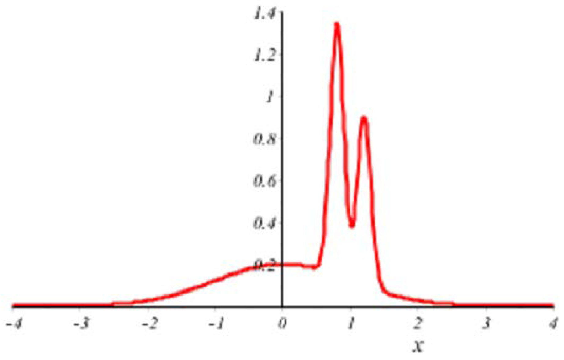
| a n | | b n | 2 T T T T ( 2 n + 1 , x ) T T T ( 2 n , α ) f ( α ) x α d α 2 d x 1 / 2 + T T T ( 2 n , x ) T T T ( 2 n + 1 , α ) f ( α ) x α d x 2 d α 1 / 2 2 π | a n | | b n | 2 T ω ( T ) T T | f ( α ) ω ( α ) | 2 d α 1 / 2 3 T π n 2 ω ( T ) T T | f ( α ) ω ( α ) | 2 d α 1 / 2 .

4. The Proof of Theorem 1

Proof. 
Using (2)–(5), one has:
( S K f ) ( x ) = C ( n ) F N f T ( x ) + k = 1 5 T T M k ( n ) ( x , α ) f T ( α ) x α d α ,
in which:
C ( n ) = 1 π 1 + ε 12 n , | ε | < 3 .
Thus, by Lemma 1 and (5),
1 2 T T T | f ( x ) ( S K f ) ( x ) | 2 d x 1 / 2 1 2 T T T | f ( x ) F n ( x ) | 2 d x 1 / 2 + 1 2 π K 1 2 T T T T T sin ( N ( x α ) ) x α f ( α ) d α 2 d x 1 / 2 + 1 π 1 + 1 2 K S a ( K , T ) 1 2 T | α | > T f ( x ) 2 d x 1 / 2 + 1 2 T | ω | > N | f ^ ( ω ) | 2 d ω 1 / 2 + 1 K 2 T ( | α | < T | f N ( α ) | 2 d α 1 / 2 + | α | > T | f ( α ) | 2 d α 1 / 2 + | ω | > N | f ^ ( ω ) | 2 d ω 1 / 2 ) + 1 π 1 + 1 2 K S a ( K , T ) = 1 + 1 K 1 2 T | α | > T f ( α ) 2 d α 1 / 2 + 1 2 T | ω | > N | f ^ ( ω ) | 2 d ω 1 / 2 + 1 K 1 2 T | α | < T | f N ( α ) | 2 d α 1 / 2 + 1 π 1 + 1 2 K S a ( K , T )
where, once again,
S a ( K , T ) = k = 1 5 1 2 T T T T T M k ( n ) ( x , α ) x α f ( α ) d α 2 d x 1 / 2 .
An explicit estimate of S a ( K , T ) is described in the Appendix using the ones involving M k ( n ) ( x , α ) , k = 1 , , 5 in Section 3.

5. An Example

Example 1 of [9] involved the Hermite series approximation of the trimodal density function:
f ( t ) = 0.5 ϕ ( t ) + 3 ϕ ( 10 ( t 0.8 ) ) + 2 ϕ ( 10 ( t 1.2 ) ) ,
in which:
ϕ ( t ) = 1 2 π e t 2 / 2 , t R ,
is the standard normal density. Figure 1 above shows that f is essentially supported in [ 3 , 3 ] . Again, from the graph of | f ^ | in Figure 4c of [9], we see that it effectively lives in [ 8 , 8 ] .
Taking T = 3 and n = 250 (so N = 31.6544 ) K = 500 , we obtain:
1 6 | t | < 3 | f ( t ) ( S 500 f ) ( t ) | 2 d t 1 / 2 < 0.02361 .
One always has:
1 2 T | t | < T | g ( t ) ( S K g ) ( t ) | 2 d t 1 / 2 s u p | t | < T | g ( t ) ( S K g ) ( t ) | ,
so, if the supremum norm is rather large, the smaller root mean square norm gives a better measure of the average size of | g ( t ) ( S K g ) ( t ) | . In our case:
s u p | t | < 3 | f ( t ) ( S 500 f ) ( t ) | < 0.0025 .
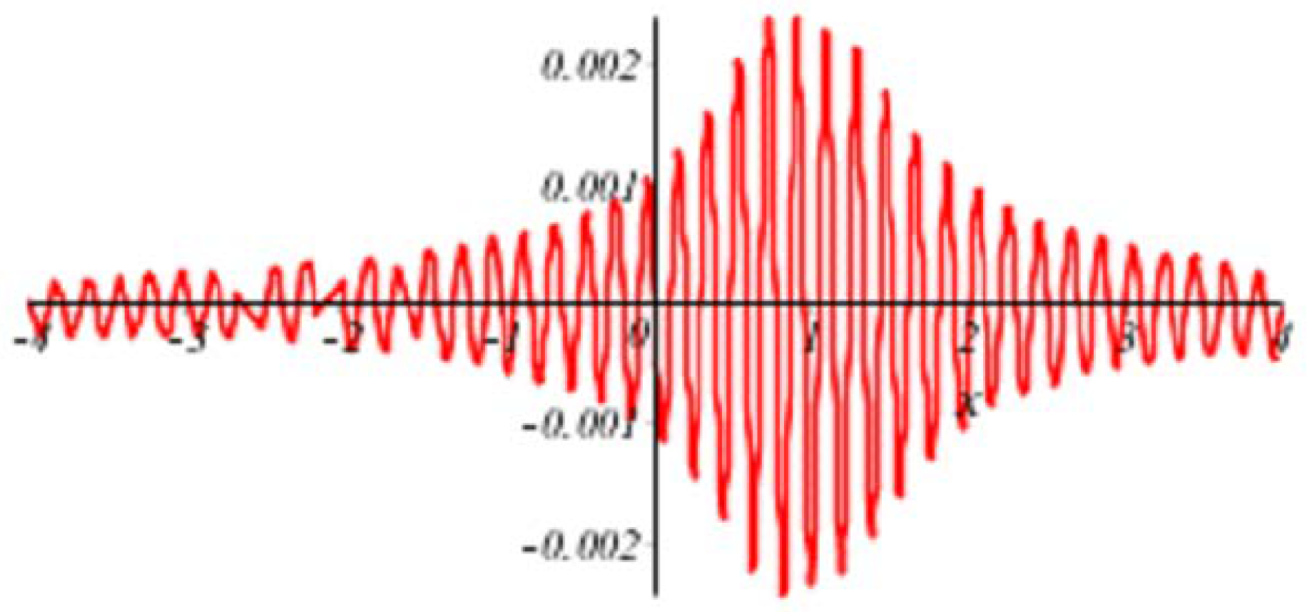
Therefore, the supremum norm is here the better measure. Nevertheless, it is the computable estimates giving (6) that lead us to Figure 2 and hence to (7).
We observe that the graph in Figure 2 is of the error function f S 500 f approximated by f S 40 f k = 41 500 f , d k d k , where d k is the Dominici approximation to b k given in Theorem 1.1 of [9].
The term involving S a ( 500 , 3 ) in (6) makes the biggest contribution to the upper bound in (1). Thus,
1.002 1 6 | t | > 3 f ( t ) 2 d t 1 / 2 < 0.00051 ,
1.002 1 6 | ω | > 31.6544 | f ^ ( ω ) | 2 d ω 1 / 2 < 0.00088
and:
1 500 1 6 | t | < 3 f ( t ) 2 d t 1 / 2 < 0.00062 ,
while:
1 π 1 + 1 1000 S a ( 500 , 3 ) < 0.02161 .
For the convenience of the reader, we have gathered together in the Appendix the terms that make up S a ( n , T ) .

Acknowledgments

We are grateful for the comments of the reviewers and Editor. They have helped us to improve the paper. The research was supported by the Natural Sciences and Engineering Council of Canada (NSERC) Grant MLH, RGPIN-2014-04621.

Author Contributions

The authors Mei Ling Huang, Ron Kerman and Susanna Spektor carried out this work and drafted the manuscript together. All authors read and approved the final manuscript.

Conflicts of Interest

The authors declare no conflict of interest.

Appendix A

Take the indicated multiples of the terms T T | f ( α ) | d α , etc., and then add them to get an estimate of the Sansone sum, S a ( K , T ) , in Formula (6).
T T | f ( α ) | d α : T 2 48 5 N 3 + T 3 384 9 N 4 + 1 8 N 3 + T 6 3 ( 4 n + 1 ) ( 4 n + 3 ) + T 6 3 ( 4 n + 3 ) + T 5 288 11 N 3 4 n + 3 + T 10 3 , 870 , 720 21 4 n + 3 N 6 + T 6 36 13 N 2 4 n + 3 + T 8 720 17 N 4 4 n + 3 ;
T T | f ( α ) α | d α : T 48 3 N 3 + 3 T 2 128 5 N 4 + 1 3 ( 4 n + 3 ) + 1 3 ( 4 n + 1 ) ( 4 n + 3 ) + T 4 144 9 N 3 4 n + 3 + 7 T 9 3 , 870 , 720 19 4 n + 3 N 6 ;
T T | f ( α ) α 2 | d α : 1 48 N 3 + T 128 3 N 4 + 1 2 N 2 ( 4 n + 1 ) + T 3 288 7 ( 4 n + 1 ) N 3 + 21 T 8 3 , 870 , 720 17 4 n + 3 N 6 ;
T T | f ( α ) α 3 | d α : 1 384 N 4 + T 3 48 7 N 2 4 n + 1 + 1 2 N 2 ( 4 n + 3 ) + T 2 288 5 ( 4 n + 1 ) N 3 + 35 T 7 3 , 870 , 720 15 4 n + 3 N 6 + T 3 36 7 N 2 4 n + 3 ;
T T | f ( α ) α 4 | d α : T 144 5 N 3 4 n + 1 + T 2 16 5 N 2 4 n + 1 + 35 T 6 3 , 870 , 720 13 N 6 ( 4 n + 3 ) ;
T T | f ( α ) α 5 | d α : 1 288 N 3 4 n + 1 + T 16 3 N 2 4 n + 1 + 21 T 5 3 , 870 , 720 11 N 6 ( 4 n + 3 ) + T 3 720 7 ( 4 n + 3 ) N 4 ;
T T | f ( α ) α 6 | d α : 1 48 N 2 4 n + 1 + 7 T 4 3 , 870 , 720 9 4 n + 3 N 6 ;
T T | f ( α ) α 7 | d α : T 3 3 , 870 , 720 7 4 n + 3 N 6 ;
T T | f ( 1 ) ( α ) | d α : 1 2 N 2 + 1 4 N 3 + T 2 6 5 ( 4 n + 1 ) ( 4 n + 3 ) + T 2 6 5 ( 4 n + 3 ) ;
T T | f ( 1 ) ( α ) α | d α : T 6 3 ( 4 n + 1 ) ( 4 n + 3 ) + T 6 3 ( 4 n + 3 ) + T 3 6 7 N 2 4 n + 3 ;
T T | f ( 1 ) ( α ) α 2 | d α : 1 6 ( 4 n + 1 ) ( 4 n + 3 ) + 1 6 ( 4 n + 3 ) ;
T T | f ( 1 ) ( α ) α 3 | d α : 1 6 ( 4 n + 1 ) N 2 ;
ω ( α ) = α 2 α 4 18 + 1 1 π 1 / 2 + 2 187 | α | 17 / 2 n 1 / 4 ,
T T | f ( α ) α | 2 d α 1 / 2 : π T 5 / 2 6 2 N 4 n + 3 + π T 1 / 2 4 N 2 ;
T T | f ( α ) α 2 | 2 d α 1 / 2 : 2 π 8 N 2 T 1 / 2 ;
T T | f ( α ) α 3 | 2 d α 1 / 2 : π T 1 / 2 6 2 ( 4 n + 1 ) N + 2 π T 5 / 2 9 ( 4 n + 1 ) ( 4 n + 3 ) + 2 3 π 2 3 2 1 / 4 T 1 / 2 ω ( T ) n 4 n + 1 + 1 24 π 3 2 3 2 1 / 4 T 1 / 2 ω ( T ) n 4 n + 3 ;
T T f N ( α ) 2 d α 1 / 2 : 2 π 8 N 2 T 3 / 2 ;
T T | f N ( α ) α 4 | 2 d α 1 / 2 : 2 π T 1 / 2 12 N 4 n + 3 ,
where f N = ( f ^ ξ ( N , N ) ) = 1 π sin N ( t s ) t s f ( s ) d s ;
T T | f ( α ) ω ( α ) | 2 d α 1 / 2 : 2 3 π 1 / 2 T 5 / 2 3 2 1 / 4 1 n 4 n + 1 + 1 24 2 π 3 / 2 T 5 / 2 3 2 1 / 4 1 n 4 n + 3 + 2 π T 1 / 2 1 n 2 ω ( T ) ;
T T | f N ( α ) ω ( α ) | 2 d α 1 / 2 : 4 2 π 1 / 2 T 1 / 2 3 2 1 / 4 1 n + 1 12 2 π 3 / 2 T 5 / 2 3 2 1 / 4 1 n ;
| f ( T ) | + | f ( T ) | : 1 2 N 2 + T 8 N 3 1 + 1 3 + T 2 6 ( 4 n + 1 ) ( 4 n + 3 ) 1 + 1 3 + 1 5 + T 3 6 N 2 4 n + 1 + T 2 6 ( 4 n + 3 ) 1 + 1 3 + 1 5 + T 3 6 7 N 2 4 n + 3 ;
| α | > T | f ( α ) 2 | d α 1 / 2 : 2 2 π 1 / 2 T 1 / 2 3 2 1 / 4 ω ( T ) n + 2 π T 7 / 2 12 N 4 n + 3 + 1 24 2 π 3 / 2 T 1 / 2 3 2 1 / 4 ω ( T ) n ;
| ω | > N | f ^ ( ω ) 2 | d ω 1 / 2 : 2 2 π 1 / 2 T 1 / 2 3 2 1 / 4 ω ( T ) n + 2 π T 7 / 2 12 N 4 n + 3 + 1 24 2 π 3 / 2 T 1 / 2 3 2 1 / 4 ω ( T ) n .

References

  1. Silverman, B.W. Density Estimation, for Statistics and Data Analysis; Chapman and Hall: New York, NY, USA, 1986. [Google Scholar]
  2. Yang, J.; Reeves, A. Bottom-up visual image processing probed with weighted polynomials. Neural Netw. 1995, 8, 669–691. [Google Scholar] [CrossRef]
  3. Barlow, R.E.; Proschan, F. Mathematical Theory of Reliability; SIAM: Philadelphia, PA, USA, 1996. [Google Scholar]
  4. Li, Q.; Racine, J.S. Nonparametric Econometrics; Theory and Practice; Princeton University Press: Oxford, UK, 2007. [Google Scholar]
  5. Koenker, R. Quantile Regression; Cambridge University Press: New York, NY, USA, 2005. [Google Scholar]
  6. Scott, D.W. Multivariate Density Estimation, Theory, Practice, and Visualization, 2nd ed.; Wiley: New York, NY, USA, 2015. [Google Scholar]
  7. Hastie, T.; Tibshirani, R.; Friedman, J. The Elememts of Statistical Learning, Dat Mining, Inference, and Prediction; Springer: New York, NY, USA, 2001. [Google Scholar]
  8. Härdle, W.; Kerkyacharian, G.; Picard, D.; Tsybakov, A. Wavelets, Approximation, and Statistical Applications; Springer: New York, NY, USA, 1998. [Google Scholar]
  9. Kerman, R.; Huang, M.L.; Brannan, M. Error estimates for Dominici’s Hermite function asymptotic formula and some applications. ANZIAM J. 2009, 50, 550–561. [Google Scholar] [CrossRef]
  10. Boyd, J.P. Asymptotic coefficients of Hermite function series. J. Comput. Phys. 1984, 54, 382–410. [Google Scholar] [CrossRef]
  11. Sansone, G. Orthogonal Functions; Pure and Applied Mathematics; Interscience Publishers, Inc.: New York, NY, USA, 1959. [Google Scholar]
  12. Uspensky, J.V. On the development of arbitrary functions in series of Hermite and Laquerre polynomials. Ann. Math. 1927, 28, 593–619. [Google Scholar] [CrossRef]
  13. Bedrosian, E. A product theorem for Hilbert transform. Proc. IEEE 1959, 51, 868–869. [Google Scholar] [CrossRef]
  14. Wiener, N. The Fourier Integral and Certain of Its Applications; Cambridge University Press: New York, NY, USA, 1933. [Google Scholar]
Figure 1. Trimodal density function.
Mathematics 06 00064 g001
Figure 2. Error function of the Hermite series approximation up to 40 terms with Dominici approximation in the next 460 terms.
Mathematics 06 00064 g002

