Quiver Gauge Theories: Finitude and Trichotomoty

Abstract

D-brane probes, Hanany-Witten setups and geometrical engineering stand as a trichotomy of standard techniques of constructing gauge theories from string theory. Meanwhile, asymptotic freedom, conformality and IR freedom pose as a trichotomy of the beta-function behaviour in quantum field theories. Parallel thereto is a trichotomy in set theory of finite, tame and wild representation types. At the intersection of the above lies the theory of quivers. We briefly review some of the terminology standard to the physics and to the mathematics. Then, we utilise certain results from graph theory and axiomatic representation theory of path algebras to address physical issues such as the implication of graph additivity to finiteness of gauge theories, the impossibility of constructing completely IR free string orbifold theories and the unclassifiability of $\mathcal{N}<2$ Yang-Mills theories in four dimensions.

1. Introduction

In a quantum field theory (QFT), it has been known since the 1970s (e.g., [1]) that the behaviour of physical quantities such as mass and coupling constant are sensitive to the renormalization and evolve according to momentum scale as dictated by the so-called renormalisation flows. In particular, the correlation (Green’s) functions, which encode the physical information relevant to Feynman’s perturbative analysis of the theory and hence unaffected by such flows, obey the famous Callan–Symanzik equations. These equations assert the existence two universal functions $\beta \left(\lambda \right)$ and $\gamma \left(\lambda \right)$ shifting according to the coupling and field renormalisation in such a way so as to compensate for the renormalisation scale.

A class of QFTs has lately received much attention, particularly among the string theorists. These are the so-named finite theories. These theories are extremely well-behaved and no divergences can be associated with the coupling in the ultraviolet; they were thus once embraced as the solution to ultraviolet infinities of QFTs. Four-dimensional finite theories are restricted to supersymmetric gauge theories (or Super-Yang-Mills, SYMs), of which divergence cancelation is a general feature, and have a wealth of interesting structure. $\mathcal{N}=4$ SYM theories have been shown to be finite to all orders (e.g., [2,3]), whereas, for $\mathcal{N}=2$, the Adler–Bardeen Theorem guarantees that no higher than 1-loop corrections exist for the $\beta$-function [4]. Finally, for the unextended $\mathcal{N}=1$ theories, the vanishing at 1-loop implies that for 2-loops [5].

When a conformal field theory (CFT) with vanishing $\beta$-function also has the anomalous dimensions vanishing, the theory is in fact a finite theory. This class of theories is without divergence and scale—and here we enter the realm of string theory. Recently, many attempts have been undertaken in the construction of such theories as low-energy limits of the world-volume theories of D-brane probes on spacetime singularities [6,7,8,9,10] or of brane setups of the Hanany-Witten type [11,12,13,14]. The construction of these theories not only supplies an excellent check for string theoretic techniques, but also, vice versa, facilitate the incorporation of the Standard Model into string unifications. These finite (super-)conformal theories in four dimensions still remain a topic of fervent pursuit.

Almost exactly concurrent with these advances in physics was a host of activities in mathematics. Inspired by problems in linear representations of partially ordered sets over a field [15,16,17,18,19], elegant and graphical methods have been developed in attacking standing problems in algebra and combinatorics such as the classification of representation types and indecomposables of finite-dimensional algebras.

In 1972, Gabriel introduced the concept of a “Köcher” in [16]. This is what is known to our standard parlance today as a “Quiver”. What entailed was a plethora of exciting and fruitful research in graph theory, axiomatic set theory, linear algebra and category theory, among many other branches. In particular, one result that has spurred interest is the great limitation imposed on the shapes of the quivers once the concept of finite representation type has been introduced.

It may at first glance seem to the reader that these two disparate directions of research in contemporary physics and mathematics may never share conjugal harmony. However, following the works of [7,8,9], those amusing quiver diagrams have surprisingly—or perhaps not too much so, considering how that illustrious field of String Theory has of late brought such enlightenment upon physics from seemingly most esoteric mathematics—taken a slight excursion from the reveries of the abstract, and manifested themselves in SYM theories emerging from D-branes probing orbifolds. The gauge fields and matter content of the said theories are conveniently encoded into quivers and further elaborations upon relations to beyond orbifold theories have been suggested in [10,20].

It is therefore natural for one to pause and step back awhile, and regard the string orbifold theory from the perspective of a mathematician, and the quivers, from that of a physicist. However, due to his inexpertise in both, the author could call himself neither. Therefore, we are compelled to peep at the two fields as outsiders, and from afar attempt to make some observations on similarities, obtain some vague notions of the beauty, and speculate upon some underlying principles. This is then the purpose of this note: to perceive, with a distant and weak eye; to inform, with a remote and feeble voice.

The organisation of the paper is as follows. Though the main results are given in Section 4, we begin with some preliminaries from contemporary techniques in string theory on constructing four dimensional super-Yang-Mills, focusing on what each interprets finitude to mean: Section 2.1 on D-brane probes on orbifold singularities, Section 2.2 on Hanany-Witten setups and Section 2.3 on geometrical engineering. Then, we move to the other direction and give preliminaries in the mathematics, introducing quiver graphs and path algebras in Section 3.1, classification of representation types in Section 3.2 and how the latter imposes constraints on the former in Section 3.3. The physicist may thus liberally neglect Section 2 and the mathematician, Section 3. Finally, in Section 4, we shall see how those beautiful theorems in graph theory and axiomatic set theory may be used to give surprising results in constructing gauge theories from string theory.

Nomenclature

Unless the contrary is stated, we shall throughout this paper adhere to the convention that k is a field of characteristic zero (and hence infinite), that Q denotes a quiver and kQ, the path algebra over the field k associated thereto, that rep(X) refers to the representation of the object X, and that irrep(Γ) is the set of irreducible representations of the group Γ. Moreover, sans serif type setting will be reserved for categories, calligraphic $\mathcal{N}$ is used to denote the number of supersymmetries and $^$, to distinguish the Affine Lie Algebras or Dynkin graphs. Finally, we emphasize that for all quivers discussed in the paper, we do not consider any relations placed in the path algebra; it would be interesting to consider how adding relations generalizes the correspondence. In addition, in graph theory, “directed graph” is usually taken to mean that there is at most one edge from one vertex to another. Since our quivers allow more edges between vertices, one should strictly use “directed pseudographs”, but, for simplicity, we will use “quiver” and “directed graph” inter-changeably.

2. Preliminaries from the Physics

The Callan–Symanzik equation of a QFT dictates the behaviour, under the renormalisation group flow, of the n-point correlator $G^{\left(n\right)}(\left\{\varphi \left(x_i\right)\right\};M,\lambda )$ for the quantum fields $\varphi \left(x\right)$, according to the renormalisation of the coupling $\lambda$ and momentum scale M (see e.g., [1], whose conventions we shall adopt):

$$\left[M\frac{\partial }{\partial M}+\beta \left(\lambda \right)\frac{\partial }{\partial \lambda }+n\gamma \left(\lambda \right)\right]G^{\left(n\right)}(\left\{\varphi \left(x_i\right)\right\};M,\lambda )=0.$$

The two universal dimensionless functions $\beta$ and $\gamma$ are known respectively as the $\beta$-function and the anomalous dimension. They determine how the shifts $\lambda \to \lambda +\delta \lambda$ in the coupling constant and $\varphi \to (1+\delta \eta )\varphi$ in the wave function compensate for the shift in the renormalisation scale M:

$$\beta \left(\lambda \right):=M\frac{\delta \lambda }{\delta M}\gamma \left(\lambda \right):=-M\frac{\delta \eta }{\delta M}.$$

Three behaviours are possible in the region of small $\lambda$: (1) $\beta \left(\lambda \right)>0$; (2) $\beta \left(\lambda \right)<0$; and (3) $\beta \left(\lambda \right)=0$. The first has good IR behaviour and admits valid Feynman perturbation at large-distance, and the second possesses good perturbative behaviour at UV limits and is asymptotically free. The third possibility is where the coupling constants do not flow at all and the renormalised coupling is always equal to the bare coupling. The only possible divergences in these theories are associated with field-rescaling which cancel automatically in physical S-matrix computations. It seems that to arrive at these well-tamed theories, some supersymmetry (SUSY) is needed so as to induce the cancelation of boson-fermion loop effects (Proposals for non-supersymmetric finite theories in four dimensions have been recently made in [8,9,21,22]; to their techniques, we shall later turn briefly.). These theories are known as the finite theories in QFT.

Of particular importance are the finite theories that arise from conformal field theories which generically have, in addition to the vanishing $\beta$-functions, also zero anomalous dimensions. Often, this subclass belongs to a continuous manifold of scale invariant theories and is characterised by the existence of exactly marginal operators and whence dimensionless coupling constants, the set of mappings among which constitutes the duality group à la Montonen-Olive of $\mathcal{N}=4$ SYM, a hotly pursued topic.

A remarkable phenomenon is that, if there is a choice of coupling constants such that all $\beta$-functions as well as the anomalous dimensions (which themselves do vanish at leading order if the manifold of fixed points include the free theory) vanish at first order, then the theory is finite to all orders (references in [12]). A host of finite theories arise as low energy effective theories of String Theory. It will be under this light that our discussions proceed. There are three contemporary methods of constructing (finite, super) gauge theories: (1) geometrical engineering; (2) D-branes probing singularities and (3) Hanany-Witten brane setups. Discussions on the equivalence among and extensive reviews for them have been in wide circulation (e.g., [23,24]). Therefore, we shall not delve too far into their account; we shall recollect from them what each interprets finitude to mean.

2.1. D-Brane Probes on Orbifolds

When placing n D3-branes on a space-time orbifold singularity ${\mathrm{₵}}^m/\Gamma$, out of the parent $\mathcal{N}=4$ $SU\left(n\right)$ SYM, one can fabricate a ${\displaystyle \prod _i}U\left(N_i\right)$ gauge theory with irrep$(\Gamma ):=\left\{{\mathbf{r}}_i\right\}$ and ${\displaystyle \sum _i}{N}_{i}dim{\mathbf{r}}_i=n$ [9]. The resulting SUSY in the four-dimensional worldvolume is $\mathcal{N}=2$ if the orbifold is ${\mathrm{₵}}^2/\{\Gamma \subset SU\left(2\right)\}$ as studied in [7], $\mathcal{N}=1$ if ${\mathrm{₵}}^3/\{\Gamma \subset SU\left(3\right)\}$ as in [10] and non-SUSY if ${\mathrm{₵}}^3/\{\Gamma \subset SU\left(4\right)\}$ as in [22]. The subsequent matter fields are $a_{ij}^{\mathbf{4}}$ Weyl fermions ${\mathsf{\Psi }}_{f_{ij}=1,\dots ,a_{ij}^{\mathbf{4}}}^{ij}$ and $a_{ij}^{\mathbf{6}}$ scalars ${\mathsf{\Phi }}_{f_{ij}}^{ij}$ with $i,j=1,\dots ,n$ and $a_{ij}^{\mathcal{R}}$ defined by

$$\mathcal{R}\otimes {\mathbf{r}}_i={\displaystyle \underset{j}{⨁}}{a}_{ij}^{\mathcal{R}}{\mathbf{r}}_j$$

(1)

respectively for $\mathcal{R}=4,6$. It is upon these matrices $a_{ij}$, which we call bifundamental matter matrices that we shall dwell. They dictate how many matter fields transform under the $(N_i,{\overline{N}}_j)$ of the product gauge group. It was originally pointed out in [7] that one can encode this information in quiver diagrams where one indexes the vector multiplets (gauge) by nodes and hypermultiplets (matter) by links in a (finite) graph so that the bifundamental matter matrix defines the (possibly oriented) adjacency matrix for this graph. In other words, one draws $a_{mn}$ number of arrows from node m to n. Therefore, to each vertex i is associated a vector space $V_i$ and a semisimple component $SU\left(N_i\right)$ of the gauge group acting on $V_i$. Moreover, an oriented link from $V_1$ to $V_2$ represents a complex field transforming under hom($V_1,V_2$). We shall see in Section 3.1 what all this means.

When we take the dimension of both sides of (1), we obtain the matrix equation

$$dim\left(\mathcal{R}\right)r_i=a_{ij}^{\mathcal{R}}{r}_j,$$

(2)

where $r_i:=dim{\mathbf{r}}_i$. As discussed in [9,10], the remaining SUSY must be in the commutant of $\Gamma$ in the $SU\left(4\right)$ R-symmetry of the parent $\mathcal{N}=4$ theory. In the case of $\mathcal{N}=2$, this means that $4=1+1+2$ and, by SUSY, $6=1+1+2+2$, where the 1 is the principal (trivial) irrep and 2, a two-dimensional irrep. Therefore, due to the additivity and orthogonality of group characters, it was thus pointed out (cit. ibid.) that one only needs to investigate the fermion matrix $a_{ij}^4$, which is actually reduced to $2{\delta }_{ij}+a_{ij}^2$. Similarly, for $\mathcal{N}=1$, we have ${\delta }_{ij}+a_{ij}^3$. It was subsequently shown that Equation (2) necessitates the vanishing of the $\beta$-function to one loop. Summarising these points, we state the condition for finitude from the orbifold perspective:

$$\begin{array}{cc}\mathrm{SUSY}& \mathrm{Finitude}\\ \mathcal{N}=2& 2r_i=a_{ij}^2{r}_j\\ \mathcal{N}=1& 3r_i=a_{ij}^3{r}_j\\ \mathcal{N}=0& 4r_i=a_{ij}^4{r}_j\end{array}$$

(3)

In fact, it was shown in [9,25], that the 1-loop $\beta$-function is proportional to $d{r}_i-a_{ij}^d{r}_j$ for $d=4-\mathcal{N}$ whereby the vanishing thereof signifies finitude, exceeding zero signifies asymptotical freedom and IR free otherwise (As a cautionary note, these conditions are necessary but may not be sufficient. In the cases of $\mathcal{N}<2$, one needs to check the superpotential. However, throughout the paper, we shall focus on the necessity of these conditions. Moreover, when $calN=0$, without the protection of supersymmetry, the QFT is more complicated. It is not immediately clear that the beta-function vanishes to all orders and the theory remains finite, thus the finiteness here will be taken to be the weaker meaning of vanishing of the beta-function to leading order.). We shall call this expression $d{\delta }_{ij}-a_{ij}^d$ the discriminant function since its relation with respect to zero (once dotted with the vector of labels) discriminates the behaviour of the QFT. This point shall arise once again in Section 4.

2.2. Hanany-Witten

In brane configurations of the Hanany-Witten type [11], D-branes are stretched between sets of NS-branes, the presence of which break the SUSY afforded by the 32 supercharges of the type II theory. In particular, parallel sets of NS-branes break one-half SUSY, giving rise to $\mathcal{N}=2$ in four dimensions [11] whereas rotated NS-branes [26] or grids of NS-branes (the so-called Brane Box Models) [12,13,14] break one further half SUSY and gives $\mathcal{N}=1$ in four dimensions.

The Brane Box Models (BBM) (and possible extensions to brane cubes) provide an intuitive and visual realisation of SYM. They generically give rise to $\mathcal{N}=1$, with $\mathcal{N}=2$ as a degenerate case. Effectively, the D-branes placed in the boxes of NS-branes furnish a geometrical way to encode the representation properties of the finite group $\Gamma$ discussed in Section 2.1. The bi-fundamentals, and hence the quiver diagram, are constructed from oriented open strings connecting the D-branes according to the rule given in [13]:

$$\mathbf{3}\otimes r_i=\underset{j\in \begin{array}{c}\mathrm{N},\mathrm{E},\mathrm{SW}\\ \mathrm{Neighbours}\end{array}}{⨁}{r}_j,$$

where N, E and SW denote the up (north), right (east) and bottom-left (south-west) directions. This is of course (1) in a different guise and we clearly see the equivalence between this and the orbifold methods of Section 2.1.

Now in [11], for the classical setup of stretching a D-brane between two NS-branes, the asymptotic bending of the NS-brane controls the evolution of the gauge coupling (since the inverse of which is dictated by the distance between the NS-branes). NS-branes bending towards each other gives an IR free theory (case (1) defined above for the $\beta$-functions), while bending away gives an UV free (case (2)) theory. No bending thus indicates the non-evolution of the $\beta$-function and thus finiteness; this is obviously true for any brane configurations, intervals, boxes or cubes. We quote [12] verbatim on this issue: Given a brane configuration which has no bending, the corresponding field theory which is read off from the brane configuration by using the rules of [13] is a finite theory.

Discussions on bending have been treated in [27,28] while works towards the establishment of the complete correspondence between Hanany-Witten methods and orbifold probes (to beyond the Abelian case) are well under way [23]. In this light, we would like to take this opportunity to point out that the anomaly cancellation Equations (2)–(4) of [27] which discusses the implication of tadpole-cancelation to BBM in excellent detail, are precisely in accordance with (1). In particular, what they referred to as the Fourier transform to extract the rank matrix for the ${\mathrm{Z}\mathrm{Z}}_k\times {\mathrm{Z}\mathrm{Z}}_{k^{\prime }}$ BBM is precisely the orthogonality relations for finite group characters (which in the case of the Abelian groups conveniently reduce to roots of unity and hence Fourier series). The generalization of these equations for non-Abelian groups should be immediate. We see indeed that there is a close intimacy between the techniques of the current subsection with Section 2.1; let us now move to a slightly different setting.

2.3. Geometrical Engineering

On compactifying Type IIA string theory on a non-compact Calabi–Yau threefold, we can geometrically engineer [25,29,30] an $\mathcal{N}=2$ SYM. More specifically, when we compactify Type IIA on a K3 surface, locally modeled by an ALE singularity, we arrive at an $\mathcal{N}=2$ SYM in six dimensions with gauge group $ADE$ depending on the singularity about which D2-branes wrap in the zero-volume limit. However, if we were to further compactify on $T^2$, we would arrive at an $\mathcal{N}=4$ SYM in four dimensions. In order to kill the extraneous scalars, we require a 2-fold without cycles, namely P${}^1$, or the 2-sphere. Therefore, we are effectively compactifying our original 10-dimensional theory on a (non-compact) Calabi–Yau threefold which is an ALE (K3) fibration over P${}^1$, obtaining a pure $\mathcal{N}=2$ SYM in four dimensions with coupling $\frac{1}{g^2}$ equal to the volume of the base P${}^1$.

To incorporate matter [25,30], we let an $A_{n-1}$ ALE fibre collide with an $A_{m-1}$ one to result in an $A_{m+n-1}$ singularity; this corresponds to a Higgsing of $SU(m+n)\to SU\left(m\right)\times SU\left(n\right)$, giving rise to a bi-fundamental matter $(n,\overline{m})$. Of course, by colliding the A singular fibres appropriately (i.e., in accordance with Dynkin diagrams), this above idea can easily be generalised to fabricate generic product $SU$ gauge groups. Thus, as opposed to Section 2.1 where bi-fundamentals (and hence the quiver diagram) arise from linear maps between irreducible modules of finite group representations, or Section 2.2 where they arise from open strings linking D-branes, in the context of geometrical engineering, they originate from colliding fibres of the Calabi–Yau.

The properties of the $\beta$-function from this geometrical perspective were also investigated in [25]. The remarkable fact, using the Perron–Frobenius Theorem, is that the possible resulting SYM is highly restricted. The essential classification is that, if the $\mathcal{N}=2$ $\beta$-function vanishes (and hence a finite theory), then the quiver diagram encoding the bi-fundamentals must be the affine $\widehat{ADE}$ Dynkin Diagrams and when it is less than zero (and thus an asymptotically free theory), the quiver must be the ordinary $ADE$. We shall see later how one may graphically arrive at these results.

Having thus reviewed the contemporary trichotomy of the methods of constructing SYM from string theory fashionable of late, with special emphasis on what the word finitude means in each, we are obliged, as prompted by the desire to unify, to ask ourselves whether we could study these techniques axiomatically. After all, the quiver diagram is manifest under all these circumstances. In addition, it is these quivers, as viewed by a graph or representation theorist, that we discuss next.

3. Preliminaries from the Mathematics

We now formally study what a quiver is in a mathematical sense. There are various approaches one could take, depending on whether one’s interest lies in category theory or in algebra. We shall commence with Gabriel’s definition, which was the genesis of the excitement which ensued. Then, we shall introduce the concept of path algebras and representation types as well as a host of theorems that limit the shapes of quivers depending on those type. As far as convention and nomenclature are concerned, Section 3.1 and Section 3.2 will largely follow [15,31,32].

3.1. Quivers and Path Algebras

In his two monumental papers [16,17], Gabriel introduced the following concept:

Definition 1.

A quiver is a pair $Q=(Q_0,Q_1)$, where $Q_0$ is a set of vertices and $Q_1$, a set of arrows such that each element $\alpha \in Q_1$ has a beginning $s\left(\alpha \right)$ and an end $e\left(\alpha \right)$ which are vertices, i.e., $\{s\left(\alpha \right)\in Q_0\}\stackrel{\alpha }{\to }\{e\left(\alpha \right)\in Q_0\}$.

In other words, a quiver is a (generically) directed graph, possibly with multiple arrows and loops. We shall often denote a member $\gamma$ of $Q_1$ by the beginning and ending vertices, as in $x\stackrel{\gamma }{\to }y$.

Given such a graph, we can generalise $Q_{0,1}$ by defining a path of length m to be the formal composition $\gamma ={\gamma }_1{\gamma }_2\cdots {\gamma }_m:=(i_0\stackrel{{\gamma }_1}{\to }{i}_1\cdots \stackrel{{\gamma }_m}{\to }{i}_m)$ with ${\gamma }_j\in Q_1$ and $i_j\in Q_0$ such that $i_0=s\left({\gamma }_1\right)$ and $i_t=s\left({\gamma }_{t-1}\right)=e\left({\gamma }_t\right)$ for $t=1,\dots ,m$. This is to say that we follow the arrows and trace through m nodes. Subsequently, we let $Q_m$ be the set of all paths of length m and for the identity define, for each node x, a trivial path of length zero, $e_x$, starting and ending at x. This allows us to associate $Q_0\sim {\left\{e_x\right\}}_{x\in Q_0}$ and $(i\stackrel{\alpha }{\to }j)\sim e_i\alpha =\alpha e_j$. Now $Q_m$ is defined for all non-negative m, whereby giving a gradation in Q.

Objects (We could take this word literally and indeed we shall later briefly define the objects in a Quiver Category.) may be assigned to the nodes and edges of the quiver so as to make its conception more concrete. This is done so in two closely-related ways:

• By the representation of a quiver, rep$\left(Q\right)$, we mean to associate to each vertex $x\in Q_0$ of Q, a vector space $V_x$ and to each arrow $x\to y$, a linear transformation between the corresponding vector spaces $V_x\to V_y$.
• Given a field k and a quiver Q, a path algebra $kQ$ is an algebra which as a vector space over k has its basis prescribed by the paths in Q.

There is a 1-1 correspondence between $kQ$-modules and rep$\left(Q\right)$. Given rep$\left(Q\right)=\{V_{x\in Q_0},(x\to y)\in Q_1\}$, the associated $kQ$ module is ${\displaystyle \underset{x}{⨁}}{V}_x$ whose basis is the set of paths $Q_m$. Conversely, given a $kQ$-module V, we define $V_x=e_{x}V$ and the arrows to be prescribed by the basis element u such that $u\sim e_{y}u=u{e}_x$ whereby making u a map from $V_x$ to $V_y$.

On an algebraic level, due to the gradation of the quiver Q by $Q_m$, the path algebra is furnished by

$$kQ:={\displaystyle \underset{m}{⨁}}k{Q}_m\mathrm{with}k{Q}_m:={\displaystyle \underset{\gamma \in Q_m}{⨁}}\gamma k.$$

(4)

As a k-algebra, the addition and multiplication axioms of $kQ$ are as follows: given $a={\displaystyle \sum _{\alpha \in Q_m;a_{\alpha }\in k}}\alpha a_{\alpha }$ and $b={\displaystyle \sum _{\beta \in Q_n;a_{\beta }\in k}}\beta a_{\beta }$ as two elements in $kQ$, $a+b={\displaystyle \sum _{\alpha }}\alpha (a_{\alpha }+b_{\alpha })$ and $a·b={\displaystyle \sum _{\alpha ,\beta }}\alpha \beta a_{\alpha }{b}_{\beta }$ with $\alpha \beta$ being the joining of paths (if the endpoint of one is the beginning of another; otherwise, it is defined to be 0).

This correspondence between path algebras and quiver representations gives us the flexibility of freely translating between the two, an advantage we shall later graciously take. As illustrative examples of concepts thus far introduced, we have drawn two quivers in Figure 1.

In example (I), $Q_0=\{1,2\},Q_1=\{\alpha ,\beta \}$ and $Q_{m>1}=\left\{\right\}$. The path algebra is then the so-called Kronecker Algebra:

$$kQ=e_{1}k\oplus e_{2}k\oplus \alpha k\oplus \beta k=\left[\begin{array}{cc}k& k^2\\ 0& k.\end{array}\right].$$

On the other hand, for example (II), $Q_{m\in \{0,1,2,\dots \}}=\left\{{\beta }^m\right\}$ and the path algebra becomes ${\displaystyle \underset{m}{⨁}}{\beta }^{m}k=k\left[\beta \right]$, the infinite dimensional free algebra of polynomials of one variable over k.

In general, $kQ$ is finitely generated if there exists a finite number of vertices and arrows in Q and $kQ$ is finite-dimensional if there do not exist any oriented cycles in Q.

To specify the quiver even further, one could introduce labeling schemes for the nodes and edges; to do so, we need a slight excursion to clarify some standard terminology from graph theory.

Definition 2.

The following are common categorisations of graphs:

• A labeled graph is a graph which has, for each of its edges $(i\stackrel{\gamma }{\to }j)$, a pair of positive integers $(a_{ij}^{\gamma },a_{ji}^{\gamma })$ associated thereto;
• A valued graph is a labeled graph for which there exists a positive integer $f_i$ for each node i, such that $a_{ij}^{\gamma }{f}_j=a_{ji}^{\gamma }{f}_i$ for each arrow (Thus, a labeled graph without any cycles is always a valued graph since we have enough degrees of freedom to solve for a consistent set of $f_i$ whereas cycles would introduce extra constraints. (Of course, there is no implicit summation assumed in the equation.)).
• A modulation of a valued graph consists of an assignment of a field $k_i$ to each node i, and a $k_i-k_j$ bi-module $M_{ij}^{\gamma }$ to each arrow $(i\stackrel{\gamma }{\to }j)$ satisfying

  (a) 

  $M_{ij}^{\gamma }\cong {hom}_{k_i}(M_{ij}^{\gamma },k_i)\cong {hom}_{k_j}(M_{ij}^{\gamma },k_j)$;

  (b) 

  ${dim}_{k_i}(M_{ij}^{\gamma })=a_{ij}^{\gamma }.$

• A modulated quiver is a valued graph with a modulation (and orientation).

We shall further adopt the convention that we omit the label to edges if it is $(1,1)$. We note that of course according to this labeling, the matrices $a_{ij}$ are almost what we call adjacency matrices. In the case of unoriented single-valence edges between say nodes i and j, the adjacency matrix has $a_{ij}=a_{ji}=1$, precisely the label $(1,1)$. However, directed edges, as in Figure 2 and Figure 3, are slightly more involved. This is exemplified by $•\Rightarrow •$ which has the label $(2,1)$ whereas the conventional adjacency matrix would have the entries $a_{ij}=2$ and $a_{ji}=0$. Such a labeling scheme is of course so as to be consistent with the entries of the Dynkin–Cartan Matrices of the semi-simple Lie Algebras. To this subtlety, we shall later turn.

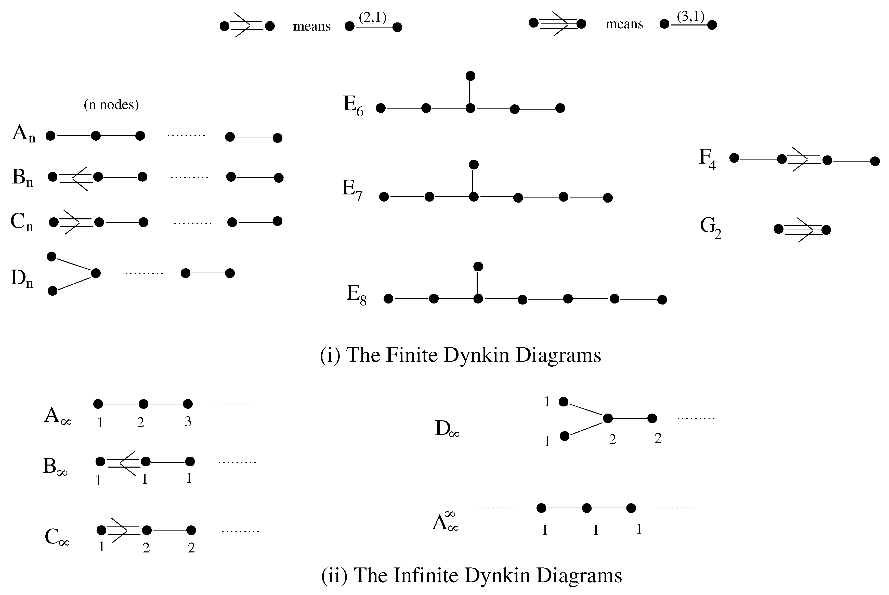
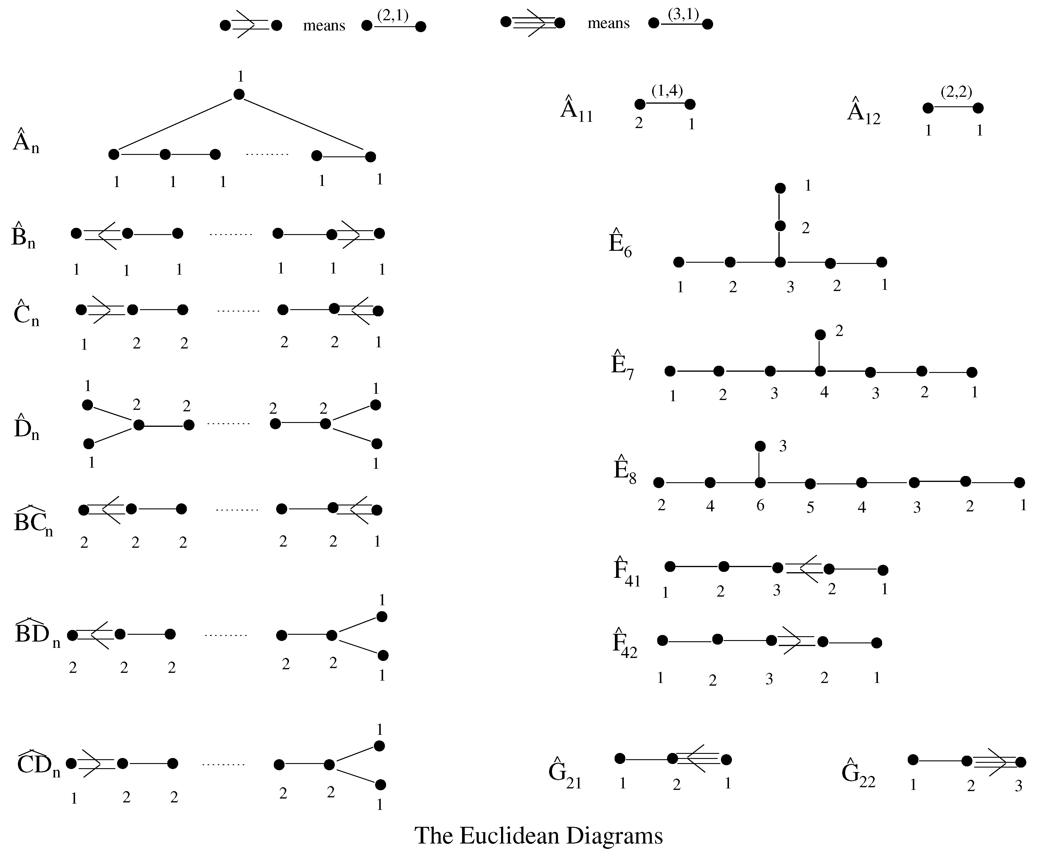
The canonical examples of labeled (some of them are valued) graphs are what are known as the Dynkin and Euclidean graphs. The Dynkin graphs are further subdivided into the finite and the infinite; the former are simply the Dynkin–Coxeter Diagrams well-known in Lie Algebras while the latter are analogues thereof but with infinite number of labeled nodes (note that the nodes are not labeled so as to make them valued graphs; we shall shortly see what those numbers signify). The Euclidean graphs are the so-called Affine Coxeter–Dynkin Diagrams (of the affine extensions of the semi-simple Lie algebras) but with their multiple edges differentiated by oriented labeling schemes. These diagrams are shown in Figure 2 and Figure 3.

How are these the canonical examples? We shall see the reason in Section 3.3 why they are ubiquitous and atomic, constituting, when certain finiteness conditions are imposed, the only elemental quivers. Before doing so, however, we need some facts from representation theory of algebras; we dwell next upon these.

3.2. Representation Type of Algebras

Henceforth, we restrict ourselves to infinite fields, as some of the upcoming definitions make no sense over finite fields. This is of no loss of generality because in physics we are usually concerned with the field $\mathrm{₵}$. When given an algebra, we know its quintessential properties once we determine its decomposables (or equivalently the irreducibles of the associated module). Therefore, classifying the behaviour of the indecomposables is the main goal of classifying representation types of the algebras.

The essential idea is that an algebra is of finite type if there are only finitely many indecomposables; otherwise, it is of infinite type. Of the infinite type, there is one well-behaved subcategory, namely the algebras of tame representation type, which has its indecomposables of each dimension coming in finitely many one-parameter families with only finitely many exceptions. Tameness in some sense still suggests classifiability of the infinite indecomposables. On the other hand, an algebra of wild type includes the free algebra on two variables, $k[X,Y]$, (the path algebra of Figure 1(II), but with two self-adjoining arrows), which indicates representations of arbitrary finite dimensional algebras, and hence unclassifiability (For precise statements of the unclassifiability of modules of two-variable free algebras as Turing-machine undecidability, cf. e.g., Thm 4.4.3 of [31,33].).

We formalise the above discussion into the following definitions:

Definition 3.

Let k be an infinite field and A, a finite dimensional algebra.

• A is of finite representation type if there are only finitely many isomorphism classes of indecomposable A-modules; otherwise, it is of infinite type;
• A is of tame representation type if it is of infinite type and for any dimension n, there is a finite set of A-$k\left[X\right]$-bimodules (Therefore, for the polynomial ring $k\left[X\right]$, the indeterminate X furnishes the parameter for the one-parameter family mentioned in the first paragraph of this subsection. Indeed, the indecomposable $k\left[X\right]$-modules are classified by powers of irreducible polynomials over k.) $M_i$ which obey the following:
  • $M_i$ are free as right $k\left[X\right]$-modules;
  • For some i and some indecomposable $k\left[X\right]$-module M, all but a finitely many indecomposable A-modules of dimension n can be written as $M_i{\otimes }_{k\left[X\right]}M$.
  If the $M_i$ may be chosen independently of n, then we say A is of domestic representation type.
• A is of wild representation type if it is of infinite representation type and there is a finitely generated A-$k[X,Y]$-bimodule M which is free as a right $k[X,Y]$-module such that the functor $M{\otimes }_{k[X,Y]}$ from finite-dimensional $k[X,Y]$-modules to finite-dimensional A-modules preserves indecomposability and isomorphism classes.

We are naturally led to question ourselves whether the above list is exhaustive. This is indeed so: what is remarkable is the so-called trichotomy theorem which says that all finite dimensional algebras must fall into one and only one of the above classification of types (For a discussion on this theorem and how similar structures arises for finite groups, e.g., [15,31] and references therein.):

Theorem 1. (Trichotomy Theorem)

For k algebraically closed, every finite dimensional algebra A is of finite, tame or wild representation types, which are mutually exclusive.

To this pigeon-hole, we may readily apply our path algebras of Section 3.1. Of course, such definitions of representation types can be generalised to additive categories with unique decomposition property. Here, by an additive category $\mathsf{B}$, we mean one with finite direct sums and an Abelian structure on $\mathsf{B}(X,Y)$, the set of morphisms from object X to Y in $\mathsf{B}$ such that the composition map $\mathsf{B}(Y,Z)\times \mathsf{B}(X,Y)\to \mathsf{B}(X,Z)$ is bilinear for $X,Y,Z$ objects in $\mathsf{B}$. Indeed, that (a) each object in $\mathsf{B}$ can be finitely decomposed via the direct sum into indecomposable objects and that (b) the ring of endomorphisms between objects has a unique maximal ideal guarantees that $\mathsf{B}$ possesses unique decomposability as an additive category [15].

The category $\mathsf{rep}\left(Q\right)$, what [34] calls the Quiver Category, has as its objects the pairs $(V,\alpha )$ with linear spaces V associated with the nodes and linear mappings $\alpha$, to the arrows. The morphisms of the category are mappings $\varphi :(V,\alpha )\to (V^{\prime },{\alpha }^{\prime })$ compatible with $\alpha$ by ${\varphi }_{e\left(l\right)}{\alpha }_l={\alpha }_l^{\prime }{\varphi }_{s\left(l\right)}$. In the sense of the correspondence between representation of quivers and path algebras as discussed in Section 3.1, the category $\mathsf{rep}\left(Q\right)$ of finite dimensional representations of Q, as an additive category, is equivalent to $\mathsf{mod}\left(kQ\right)$, the category of finite dimensional (right) modules of the path algebra $kQ$ associated with Q. This equivalence

$$\mathsf{rep}\left(Q\right)\cong \mathsf{mod}\left(kQ\right)$$

is the axiomatic statement of the correspondence and justifies why we can hereafter translate freely between the concept of representation types of quivers and associated path algebras.

3.3. Restrictions on the Shapes of Quivers

Now, we return to our quivers and in particular combine Section 3.1 and Section 3.2 to address the problem of how the representation types of the path algebra restricts the shapes of the quivers. Before doing so, let us first justify, as advertised in Section 3.1, why Figure 2 and Figure 3 are canonical. We first need a preparatory definition: we say a labeled graph $T_1$ is smaller than $T_2$ if there is an injective morphism of graphs $\rho :T_1\to T_2$ such that for each edge $(i\stackrel{\gamma }{\to }j)$ in $T_1$, $a_{ij}\le a_{\rho \left(i\right)\rho \left(j\right)}$ (and $T_1$ is said to be strictly smaller if $\rho$ can not be chosen to be an isomorphism). With this concept, we can see that the Dynkin and Euclidean graphs are indeed our archetypal examples of labeled graphs due to the following theorem:

Theorem 2

(See in [31,32]). Any connected labeled graph T is one and only one of the following:

• T is Dynkin (finite or infinite);
• There exists a Euclidean graph smaller than T.

This is a truly remarkable fact which dictates that the atomic constituents of all labeled graphs are those arising from semi-simple (ordinary and affine) Lie Algebras. The omni-presence of such meta-patterns is still largely mysterious (see e.g., [20,35] for discussions on this point).

Let us see another manifestation of the elementarity of the Dynkin and Euclidean Graphs. Again, we need some rudimentary notions.

Definition 4.

The Cartan Matrix for a labeled graph T with labels $(a_{ij},a_{ji})$ for the edges is the matrix (This definition is inspired by, but should be confused with, Cartan matrices for semisimple Lie algebras; to the latter, we shall refer to them as Dynkin–Cartan matrices. In addition, in the definition, we have summed over edges γ adjoining i and j so as to accommodate multiple edges between the two nodes each with non-trivial labels.) $c_{ij}:=2{\delta }_{ij}-{\displaystyle \sum _{\gamma }}{a}_{ij}^{\gamma }$.

We can symmetrise the Cartan matrix for valued graphs as ${\tilde{c}}_{ij}=c_{ij}{f}_j$ with $\left\{f_j\right\}$ the valuation of the nodes of the labeled graph. With the Cartan matrix at hand, let us introduce an important function on labeled graphs:

Definition 5.

A subadditive function $n\left(x\right)$ on a labeled graph T is a function taking nodes $x\in T$ to $n\in {\mathrm{Q}}^{+}$ such that ${\displaystyle \sum _i}n\left(i\right)c_{ij}\ge 0\forall j$. A subadditive function is additive if the equality holds.

It turns out that imposing the existence such a function highly restricts the possible shape of the graph; in fact, we are again led back to our canonical constituents. This is dictated by the following

Theorem 3

(Happel-Preiser-Ringel [31]). Let T be a labeled graph and $n\left(x\right)$ a subadditive function thereupon, then the following holds:

• T is either (finite or infinite) Dynkin or Euclidean;
• If $n\left(x\right)$ is not additive, then T is finite Dynkin or $A_{\infty }$;
• If $n\left(x\right)$ is additive, then T is infinite Dynkin or Euclidean;
• If $n\left(x\right)$ is unbounded then $T=A_{\infty }.$

We shall see in the next section what this notion of graph additivity [31,35] signifies for super-Yang-Mills theories. For now, let us turn to the Theorema Egregium of Gabriel that definitively restricts the shape of the quiver diagram once the finitude of the representation type of the corresponding path algebra is imposed.

Theorem 4

(Gabriel [15,16,17]). A finite quiver Q (and hence its associated path algebra over an infinite field) is of finite representation type if and only if it is a disjoint union of Dynkin graphs of type $A_n$, $D_n$ and $E_{678}$, i.e., the ordinary simply-laced $ADE$ Coxeter–Dynkin diagrams.

In the language of categories [34], where a proof of the theorem may be obtained using Coxeter functors in the Quiver Category, the above proposes that the quiver is (unions of) $ADE$ if and only if there are a finite number of non-isomorphic indecomposable objects in the category rep$\left(Q\right)$.

Once again, the graphs of Figure 2 appear, and, in fact, only the single-valence ones: that ubiquitous $ADE$ meta-pattern! We recall from discussions in Section 3.1 that only for the simply-laced (and thus the quivers do not have multiple lines between nodes) cases, viz. $ADE$ and $\widehat{ADE}$, do the labels $a_{ij}^{\gamma }$ precisely prescribe the adjacency matrices. To what type of path algebras then, one may ask, do the affine $\widehat{ADE}$ Euclidean graphs correspond? The answer is given by Nazarova as an extension to Gabriel’s Theorem.

Theorem 5

(Nazarova [15, 36]). Let Q be a connected quiver without oriented cycles and let k be an algebraically closed field; then, $kQ$ is of tame (in fact domestic) representation type if and only if Q is one of the Euclidean graphs of type ${\widehat{A}}_n$, ${\widehat{D}}_n$ and ${\widehat{E}}_{678}$, i.e., the affine $ADE$ Coxeter–Dynkin diagrams.

Can we push further? What about the remaining quivers in our canonical list? Indeed, with the introduction of modulation on the quivers, as introduced in Section 3.1, the results can be further relaxed to include more graphs; in fact, all the Dynkin and Euclidean graphs:

Theorem 6

(Tits, Bernstein-Gel’fand-Ponomarev, Dlab-Ringel, Nazarova-Ringel [19,31,34,37]). Let Q be a connected modulated quiver, then

• If Q is of finite representation type then Q is Dynkin;
• If Q is of tame representation type, then Q is Euclidean.

This is then our dualism; on the one level of having finite graphs encoding a (classifiability) infinite algebra and on another level having the two canonical constituents of all labeled graphs being partitioned by finitude versus infinitude (This is much in the spirit of that wise adage, “Cette opposition nouvelle, ‘le fini et l’infini’, ou mieux ‘l’infini dans le fini’, remplace le dualisme de l’être et du paraître: ce qui paraît, en effet, c’est seulement un aspect de l’objet et l’objet est tout entier dans cet aspect et tout entier hors de lui [38].”).

4. Quivers in String Theory and Yang-Mills in Graph Theory

We are now equipped with a small arsenal of facts; it is now our duty to expound upon them. Therefrom, we shall witness how axiomatic studies of graphs and representations may shed light on current developments in string theory.

Let us begin then, upon examining condition (3) and Definition 5, with the following

Observation 1.

The condition for finitude of $\mathcal{N}=2$ orbifold SYM theory is equivalent to the introduction of an additive function on the corresponding quiver as a labeled graph.

This condition that for the label $n_i$ to each node i and adjacency matrix $A_{ij}$, $2n_i={\displaystyle \sum _j}{a}_{ij}{n}_j$ is a very interesting constraint to which we shall return shortly. What we shall use now is Part 3 of Theorem 3 in conjunction with the above observation to deduce.

Corollary 1.

All finite $\mathcal{N}=2$ super-Yang-Mills Theories with bi-fundamental matter have their quivers as (finite disjoint unions) of the single-valence (i.e., $(1,1)$-labeled edges) cases of the Euclidean (3) or Infinite Dynkin (2) graphs.

There are a few points to make here. This is a slightly more extended list than that given in [25] which is comprised solely of the $\widehat{ADE}$ quivers. These latter cases are the ones of contemporary interest because they, in addition to being geometrically constructable (Section 2.3), are also obtainable from the string orbifold technique (In addition, in the cases of A and D also from Hanany-Witten setups [23,39].) (Section 2.1) since after all the finite discrete subgroups of $SU\left(2\right)$ fall into an $\widehat{ADE}$ classification due to McKay’s Correspondence [6,10,40]. In addition to the above well-behaved cases, we also have the infinite simply-laced Dynkin graphs: $A_{\infty },D_{\infty }$ and $A_{\infty }^{\infty }$. The usage of the Perron–Frobenius Theorem in [25] restricts one’s attention to finite matrices. The allowance for infinite graphs of course implies an infinitude of nodes and hence infinite products for the gauge group. One needs not exclude these possibilities as after all in the study of D-brane probes, Maldacena’s large N limit has been argued in [8,9,12] to be required for conformality and finiteness. In this limit of an infinite stack of D-branes, infinite gauge groups may well arise. In the Hanany-Witten picture, $A_{\infty }^{\infty }$ for example would correspond to an infinite array of NS5-branes, and $A_{\infty }$, a semi-infinite array with enough D-branes on the other side to ensure the overall non-bending and parallelism of the NS. Such cases had been considered in [26].

Another comment is on what had been advertised earlier in Section 3.1 regarding the adjacency matrices. Theorem 3 does not exclude graphs with multiple-valanced oriented labels. This issue does not arise in $\mathcal{N}=2$ which has only single-valanced and unoriented quivers. However, going beyond to $\mathcal{N}=1,0$, requires generically oriented and multiply-valanced quivers (i.e., non-symmetric, non-binary matter matrices) [10,22]; or, it is conceivable that certain theories not arising from orbifold procedures may also possess these generic traits. In this light, we question ourselves how one may identify the bi-fundamental matter matrices not with strict adjacency matrices of graphs but with the graph-label matrices $a_{ij}^{\gamma }$ of Section 3.1 so as to accommodate multiple, chiral bi-fundamentals (i.e., multi-valence, directed graphs). In other words, could Corollary 1 actually be relaxed to incorporate all of the Euclidean and infinite Dynkin graphs as dictated by Theorem 3? Thoughts on this direction, viz., how to realise Hanany-Witten brane configurations for non-simply-laced groups have been engaged but still awaits further clarification [41].

Let us now turn to Gabriel’s famous Theorem 4 and see its implications in string theory and, vice versa, what information the latter provides for graph theory. First, we make a companion statement to Observation 1:

Observation 2.

The condition for asymptotically free ($\beta <0$) $\mathcal{N}=2$ SYM theory with bi-fundamentals is equivalent to imposing a subadditive (but not additive) function of the corresponding quiver.

This may thus promptly be utilised together with Part 2 of Theorem 3 to conclude that the only such theories are ones with $ADE$ quiver, or, allowing infinite gauge groups, $A_{\infty }$ as well (and indeed all finite Dynkin quivers once, as mentioned above, non-simply-laced groups have been resolved). This is once again a slightly extended version of the results in [25].

Let us digress, before trudging on, a moment to consider what it means to encode SYM with quivers. Now, we recall that, for the quiver Q, the assignment of objects and morphisms to the category rep$\left(Q\right)$, or vector spaces and linear maps to nodes $Q_0$ and edges $Q_1$ in Q, or bases to the path algebra $kQ$, are all equivalent procedures. From the physics perspective, these assignments are precisely what we do when we associate vector multiplets to nodes and hypermultiplets to arrows as in the orbifold technique, or NS-branes to nodes and oriented open strings between D-branes to arrows as in the Hanany-Witten configurations, or singularities in Calabi–Yau to nodes and colliding fibres to arrows as in geometrical engineering. In other words, the three methods, Section 2.1, Section 2.3 and Section 3.1, of constructing gauge theories in four dimensions currently in vogue are different representations of rep$\left(Q\right)$ and are hence axiomatically equivalent as far as quiver theories are concerned.

Bearing this in mind, and in conjunction with Observations 1 and 2, as well as Theorem 4 together with its generalisations, and in particular Theorem 6, we make the following:

Corollary 2.

To an asymptotically free $\mathcal{N}=2$ SYM with bi-fundamentals is associated a finite path algebra and to a finite one, a tame path algebra. The association is in the sense that these SYM theories (or some theory categorically equivalent thereto) prescribe representations of the only quivers of such representation types.

What is even more remarkable perhaps is that, due to the Trichotomy Theorem, the path algebra associated with all other quivers must be of wild representation type. What this means, as we recall the unclassifiability of algebras of wild representations, is that these quivers are unclassifiable. In particular, if we assume that SYM with $\mathcal{N}=0.1$ and arbitrary bi-fundamental matter content can be constructed (either from orbifold techniques, Hanany-Witten, or geometrical engineering), then these theories can not be classified, in the strict sense that they are Turing undecidable and there does not exist, in any finite language, a finite scheme by which they could be listed. Since the set of SYM with bi-fundamentals is a proper subset of all SYM, the like applies to general SYM. What this signifies is that however ardently we may continue to provide more examples of say finite $\mathcal{N}=1.0$ SYM, the list can never be finished nor be described, unlike the $\mathcal{N}=2$ case where the above discussions exhaust their classification. We summarise this amusing if not depressing fact as follows:

Corollary 3.

The generic $\mathcal{N}=1.0$ SYM in four dimensions are unclassifiable in the sense of being Turing undecidable.

We emphasise again that by unclassifiable here we mean not completely classifiable because we have given a subcategory (the theories with bi-fundamentals) which is unclassifiable. In addition, we rest upon the assumption that for any bi-fundamental matter content an SYM could be constructed. Works in the direction of classifying all possible gauge invariant operators in an $\mathcal{N}=1$ SUSY Lagrangian have been pursued [42]. Our claim is much milder, as no further constraints than the possible naïve matter content are imposed; we simply state that the complete generic problem of classifying the $\mathcal{N}<2$ matter content is untractable. In [42], the problem has been reduced to manipulating a certain cohomological algebra; it would be interesting to see, for example, whether such BRST techniques may be utilised in the classification of certain categories of graphs.

Such an infinitude of gauge theories need not worry us as there certainly is no shortage of say, Calabi–Yau threefolds which may be used to geometrically engineer them. This unclassifiability is rather in the spirit of that of, for example, four-manifolds. Indeed, though we may never exhaust the list, we are not precluded from giving large exemplary subclasses which are themselves classifiable, e.g., those prescribed by the orbifold theories. Determining these theories amounts to the classification of the finite discrete subgroups of $SU\left(n\right)$.

We recall from Corollary 1 that $\mathcal{N}=2$ is given by the affine and infinite Coxeter–Dynkin graphs of which the orbifold theories provide the $\widehat{ADE}$ cases. What remarks could one make for $\mathcal{N}=0,1$, i.e., $SU(3,4)$ McKay quivers [10,22]? Let us first see $\mathcal{N}=2$ from the graph-theoretic perspective, which will induce a relationship between additivity (Theorem 3) and Gabriel-Nazarova (Theorems 4 and extensions). The crucial step in Tit’s proof of Gabriel’s Theorem is the introduction of the quadratic form on a graph [34,43]:

Definition 6.

For a labeled quiver $Q=(Q_0,Q_1)$, one defines the (symmetric bilinear) quadratic form $B\left(x\right)$ on the set x of the labels as follows:

$$B\left(x\right):={\displaystyle \sum _{i\in Q_0}}{x}_i^2-{\displaystyle \sum _{\alpha \in Q_1}}{x}_{s\left(\alpha \right)}{x}_{e\left(\alpha \right)}.$$

The subsequent work was then to show that finitude of representation is equivalent to the positive-definiteness of $B\left(x\right)$, and, in fact, as in Nazarova’s extension, that tameness is equivalent to positive-semi-definiteness. In other words, finite or tame representation type can be translated, in this context, to a Diophantine inequality which dictates the nodes and connectivity of the quiver (incidentally the very same Inequality which dictates the shapes of the Coxeter–Dynkin Diagrams or the vertices and faces of the Platonic solids in $\mathrm{I}\mathrm{R}{}^3$):

$$B\left(x\right)\ge 0\iff \widehat{ADE},ADEB\left(x\right)>0\iff ADE.$$

Now, we note that $B\left(x\right)$ can be written as $\frac{1}{2}{x}^T·c·x$, where ${\left(c\right)}_{ij}$ is de facto the Cartan Matrix for graphs as defined in Section 3.3. The classification problem thus, because $c:=2I-a$, becomes that of classifying graphs whose adjacency matrix a has maximal eigenvalue 2, or what McKay calls $C_2$-graphs in [40]. This issue was addressed in [44] and indeed the $\widehat{ADE}$ graphs emerge. Furthermore, the additivity condition ${\displaystyle \sum _j}{c}_{ij}{x}_j\ge 0\forall i$ clearly implies the constraint ${\displaystyle \sum _{ij}}{c}_{ij}{x}_i{x}_j\ge 0$ (since all labels are positive) and thereby the like on the quadratic form. Hence, we see how to arrive at the vital step in Gabriel–Nazarova through graph subadditivity.

The above discussions relied upon the specialty of the number 2. Indeed, one could translate between the graph quadratic form $B\left(x\right)$ and the graph Cartan matrix precisely because the latter is defined by $2I-a$. From a physical perspective, this is precisely the discriminant function for $\mathcal{N}=2$ orbifold SYM (i.e., $d=2$) as discussed at the end of Section 2.1. This is why $\widehat{ADE}$ arises in all these contexts. We are naturally led to question ourselves, what about general (In the arena of orbifold SYM, $d=1,2,3$, but in a broader settings, as in generalisation of McKay’s Correspondence, d could be any natural number.) d? This compels us to consider a generalised Cartan matrix for graphs (Cf. Definition in Section 3.3), given by $c_{ij}:=d{\delta }_{ij}-a_{ij}$, our discriminant function of Section 2.1. Indeed, such a matrix was considered in [45] for general McKay quivers. As a side remark, due to such an extension, Theorem 3 must likewise be adjusted to accommodate more graphs; a recent paper [46] shows an example, the so-dubbed semi-Affine Dynkin Diagrams, where a new class of labeled graphs with additivity with respect to the extended $c_{ij}$ emerge.

Returning to the generalised Cartan matrix, in [45], the McKay matrices $a_{ij}$ were obtained, for an arbitrary finite group G, by tensoring a faithful d-dimensional representation with the set of irreps: $r_d\otimes r_i={\oplus }_j{a}_{ij}{r}_j$. What was noticed was that the scalar product defined with respect to the matrix $d{\delta }_{ij}-a_{ij}$ (precisely our generalised Cartan) was positive semi-definite in the vector space $V=\left\{x_i\right\}$ of labels. In other words, ${\displaystyle \sum _{ij}}{c}_{ij}{x}_i{x}_j\ge 0$. We briefly transcribe his proof in the Appendix A. What this means for us is the following:

Corollary 4.

String orbifold theories can not produce a completely IR free (i.e., with respect to all semisimple components of the gauge group) QFT (i.e., Type (1), $\beta >0$).

To see this, suppose there existed such a theory. Then, $\beta >0$, implying for our discriminant function that ${\displaystyle \sum _j}{c}_{ij}{x}_j<0\forall i$ for some finite group. This would then imply, since all labels are positive, that ${\displaystyle \sum _{ij}}{c}_{ij}{x}_i{x}_j<0$, violating the positive semidefiniteness condition that it should always be nonnegative for any finite group according to [45]. Therefore, by reductio ad absurdum, we conclude Corollary 4.

On a more general setting, if we were to consider using the generalised Cartan matrix $d{\delta }_{ij}-a_{ij}$ to define a generalised subadditive function (as opposed to merely $d=2$), could we perhaps have an extended classification scheme? To our knowledge, this is so far an unsolved problem for indeed take the subset of these graphs with all labels being 1 and $d{n}_i={\displaystyle \sum _j}{a}_{ij}{n}_j$, these are known as d-regular graphs (the only 2-regular one is the $\widehat{A}$-series) and these are already unclassified for $d>2$. We await input from mathematicians on this point.

5. Concluding Remarks and Prospects

The approach of this writing has been bilateral. On the one hand, we have briefly reviewed the three contemporary techniques of obtaining four dimensional gauge theories from string theory, namely Hanany-Witten, D-brane probes and geometrical engineering. In particular, we focus on what finitude signifies for these theories and how interests in quiver diagrams arises. Subsequently, we approach from the mathematical direction and have taken a promenade in the field of axiomatic representation theory of algebras associated with quivers. The common ground rests upon the language of graph theory, some results from which we have used to address certain issues in string theory.

From the expression of the one-loop $\beta$-function, we have defined a discriminant function $f:=d{\delta }_{ij}-a_{ij}^d$ for the quiver with adjacency matrix $a_{ij}$ which encodes the bi-fundamental matter content of the gauge theory. The nullity (resp. negativity/positivity) of this function gives a necessary condition for the finitude (resp. IR freedom/asymptotic freedom) of the associated gauge theory. We recognise this function to be precisely the generalised Cartan matrix of a (not necessarily finite) graph and the nullity (resp. negativity) thereof, the additivity (resp. strict subadditivity) of the graph. In the case of $d=2$, such graphs are completely classified: infinite Dynkin or Euclidean if $f=0$ and finite Dynkin or $A_{\infty }$ if $f<0$. In physical terms, this means that these are the only $\mathcal{N}=2$ theories with bi-fundamental matter (Corollary 1 and Observation 2). This slightly generalises the results of [25] by the inclusion of infinite graphs, i.e., theories with infinite product gauge groups. From the mathematics alone, also included are the non-simply-laced diagrams; however, we still await progress in the physics to clarify how these gauge theories may be fabricated.

For $d>2$, the mathematical problem of their classification is so far unsolved. A subclass of these, namely the orbifold theories coming from discrete subgroups of $SU\left(n\right),$ have been addressed upto $n=4$ [7,10,22]. A general remark we can make about these theories is that, due to a theorem of Steinberg, D-brane probes on orbifolds can never produce a completely IR free QFT (Corollary 4).

From a more axiomatic stand, we have also investigated possible finite quivers that may arise. In particular, we have reviewed the correspondence between a quiver and its associated path algebra. Using the Trichotomy theorem of representation theory, that all finite dimensional algebras over an algebraically closed field are of either finite, tame or wild type, we have seen that all quivers are respectively either $ADE$, $\widehat{ADE}$ or unclassifiable. In physical terms, this means that asymptotically free and finite $\mathcal{N}=2$ SYM in four dimensions respectively exhaust the only quiver theories of respectively finite and tame type (Corollary 2). What these particular path algebras mean in a physical context, however, is yet to be ascertained. For the last type, we have drawn a melancholy note that all other theories, and, in particular, $\mathcal{N}<2$ in four dimensions, are in general Turing unclassifiable (Corollary 3).

Much work remains to be accomplished. It is the main purpose of this note, through the eyes of a neophyte, to inform readers in each of two hitherto disparate fields of gauge theories and axiomatic representations, of certain results from the other. It is hoped that future activity may be prompted.

References

- Peskin, M.; Schröder, D. An Introduction to Quantum Field Theory; Addison-Wesley: Boston, MA, USA, 1995. [Google Scholar]
- West, P. Finite Four Dimensional Supersymmetric Theories. In Problems in Unification and Supergravity; AIP Conference Proceedings, No. 116; American Institute of Physics: College Park, MD, USA, 1984. [Google Scholar]
- Ferrara, S.; Zumino, B. Supergauge invariant yang-mills theories. Nucl. Phys. B 1974, 79, 413–421. [Google Scholar] [CrossRef]
- Grisaru, M.; Siegel, W. Supergraphity:(II). Manifestly covariant rules and higher-loop finiteness. Nucl. Phys. B 1982, 201, 292–314. [Google Scholar] [CrossRef]
- Parkes, A.; West, P. Finiteness in rigid supersymmetric theories. Phy. Lett. B 1984, 138, 99–104. [Google Scholar] [CrossRef]
- Douglas, M.; Greene, B. Metrics on D-brane Orbifolds. Adv. Theor. Math. Phys. 1998, 1, 184–196. [Google Scholar] [CrossRef]
- Johnson, C.V.; Myers, R.C. Aspects of Type IIB Theory on ALE Spaces. Phys. Rev. D 1997, 55, 6382–6393. [Google Scholar] [CrossRef]
- Kachru, S.; Silverstein, E. 4D Conformal Field Theories and Strings on Orbifolds. Phys. Rev. Lett. 1998, 80, 4855–4858. [Google Scholar] [CrossRef] [Green Version]
- Lawrence, A.; Nekrasov, N.; Vafa, C. On Conformal Field Theories in Four Dimensions. Nucl. Phys. B 1998, 533, 199–209. [Google Scholar] [CrossRef]
- Hanany, A.; He, Y.-H. Non-Abelian Finite Gauge Theories. J. High Energy Phys. 1999. [Google Scholar] [CrossRef]
- Hanany, A.; Witten, E. Type IIB Superstrings, BPS monopoles, and Three-Dimensional Gauge Dynamics. Nucl. Phys. B 1997, 492, 152–190. [Google Scholar] [CrossRef]
- Hanany, A.; Strassler, M.J.; Uranga, A.M. Finite Theories and Marginal Operators on the Brane. J. High Energy Phys. 1998. [Google Scholar] [CrossRef]
- Hanany, A.; Zaffaroni, A. On the Realisation of Chiral Four-Dimensional Gauge Theories Using Branes. J. High Energy Phys. 1998. [Google Scholar] [CrossRef]
- Hanany, A.; Uranga, A. Brane Boxes and Branes on Singularities. J. High Energy Phys. 1998. [Google Scholar] [CrossRef]
- Simson, D. Linear Representations of Partially Ordered Sets and Vector Space Categories; Algebra, Logic and Applications Series; Gordon and Breach Science Publishers: London, UK, 1992; Volume 4. [Google Scholar]
- Gabriel, P. Unzerlegbare Darstellugen I. Manuscr. Math. 1972, 6, 71–103. [Google Scholar] [CrossRef]
- Gabriel, P. Indecomposable representations II. In Symposia Mathematica; Academic Press: London, UK, 1973; pp. 81–104, Volume XI (Convegno di Algebra Commutativa, INDAM, Rome, 1971). [Google Scholar]
- Gel’fand, I.M.; Ponomarev, V.A. Quadruples of Subspaces of a Finite-Dimensional Vector Space. Soviet Math. Dokl. 1971, 12, 762–765. [Google Scholar]
- Dlab, V.; Ringel, C. On Algebras of Finite Representation Type. J. Algebra 1975, 33, 306–394. [Google Scholar] [CrossRef]
- He, Y.-H.; Song, J.S. Of McKay Correspondence, Non-linear Sigma-model and Conformal Field Theory. Adv. Theor. Math. Phys. 2000, 4, 747–790. [Google Scholar] [CrossRef]
- Frampton, P.; Vafa, C. Conformal Approach to Particle Phenomenology. arXiv, 1999; arXiv:hep-th/9903226. [Google Scholar]
- Hanany, A.; He, Y.-H. A Monograph on the Classification of the Discrete Subgroups of SU(4). J. High Energy Phys. 2001. [Google Scholar] [CrossRef]
- Feng, B.; Hanany, A.; He, Y.-H. The Zk × Dk′ Brane Box Model. J. High Energy Phys. 1999. [Google Scholar] [CrossRef]
- Elitzur, S.; Giveon, A.; Kutasov, D.; Rabinovici, E.; Schwimmer, A. Brane Dynamics and N = 1 Supersymmetric Gauge Theory. Nucl. Phys. B 1997, 505, 202–250. [Google Scholar] [CrossRef]
- Katz, S.; Mayr, P.; Vafa, C. Mirror symmetry and Exact Solution of 4D N = 2 Gauge Theories I. Adv. Theor. Math. Phys. 1998, 1, 53–114. [Google Scholar] [CrossRef]
- Erlich, J.; Hanany, A.; Naqvi, A. Marginal Deformations from Branes. J. High Energy Phys. 1999. [Google Scholar] [CrossRef]
- Leigh, R.; Rozali, M. Brane Boxes, Anomalies, Bending and Tadpoles. J. High Energy Phys. Phys. Rev. D 1999, 59, 026004. [Google Scholar] [CrossRef]
- Randall, L.; Shirman, Y.; von Unge, R. Brane Boxes: Bending and Beta Functions. J. High Energy Phys. 1998. [Google Scholar] [CrossRef]
- Katz, S.; Klemm, A.; Vafa, C. Geometric Engineering of Quantum Field Theories. Nucl. Phys. B 1997, 497, 173–195. [Google Scholar] [CrossRef]
- Katz, S.; Vafa, C. Matter from Geometry. Nucl. Phys. B 1997, 497, 146–154. [Google Scholar] [CrossRef]
- Benson, D. Representations and Cohomology; Cambridge Studies in Advanced Mathematics 30; Cambridge University Press: Cambridge, UK, 1991. [Google Scholar]
- Benson, D. Modular Representation Theory: New Trends and Methods; Lecture Notes in Mathematics 1081; Springer-Verlag: Berlin, Germany, 1984. [Google Scholar]
- Baur, W. Decidability and Undecidability of Theories of Abelian Groups with Predicates for Subgroups. Compos. Math. 1975, 31, 23–30. [Google Scholar]
- Bernstein, I.N.; Gel’fand, I.M.; Ponomarev, V.A. Coxeter Functors and Gabriel’s Theorem. Rus. Math. Surv. 1973, 28, 17–32. [Google Scholar] [CrossRef]
- Gannon, T. Monstrous Moonshine and the Classification of CFT. arXiv, 1999; arXiv:math/9906167. [Google Scholar]
- Nazarova, L.A.; Ovsienko, S.A.; Roiter, A.V. Polyquivers of Finite Type (Russian). Trudy Mat. Inst. Steklov. 1978, 148, 190–194, 277. [Google Scholar]
- Nazarova, L.A.; Roiter, A.V. Polyquivers and Dynkin Schemes. Funct. Anal. Appl. 1973, 7, 252–253. [Google Scholar] [CrossRef]
- Sartre, J.-P. L’être et le Néant, Essai D’ontologie Phénonénologique; Nrf Gallimard: Paris, France, 1990. [Google Scholar]
- Kapustin, A. Dn Quivers from Branes. J. High Energy Phys. 1998. [Google Scholar] [CrossRef]
- McKay, J. Graphs, Singularities, and Finite Groups. Proc. Symp. Pure Math. 1980, 37, 183–186. [Google Scholar]
- He, Y.-H.; University of London, London, UK; Bo, F.; Zhejiang University, Hangzhou, China; Hanan, A.; Imperial College London, London, UK. Personal Communication, 2001.
- Barnich, G.; Brandt, F.; Henneaux, M. Local BRST cohomology in Einstein-Yang-Mills theory. Nucl. Phys. B 1995, 455, 357–408. [Google Scholar] [CrossRef] [Green Version]
- Donovan, P.; Freislich, M. The Representation Theory of Finite Graphs and Associated Algebras; Carleton Mathematical Lecture; Carleton University: Ottawa, ON, Canada, 1973. [Google Scholar]
- Smith, J. Some properties of the spectrum of a graph. In Proceedings of the 1969 Calgary Conference on Combinatorial Structures and Their Applications, Calgary, AL, Canada, 2–14 June 1970; pp. 403–406. [Google Scholar]
- Steinberg, R. Finite Subgroups of SU2, Dynkin Diagrams and Affine Coxeter Elements. Pac. J. Math. 1985, 118, 587–598. [Google Scholar] [CrossRef]
- McKay, J. Semi-affine Coxeter–Dynkin graphs and G ⊆ SU2(C). Can. J. Math. 1999, 51, 1226–1229. [Google Scholar] [CrossRef]
Figure 1.
Two examples of quivers with nodes and edges labeled.
Figure 2.
The Finite and Infinite Dynkin Diagrams as labeled quivers. The finite cases are the well-known Dynkin–Coxeter graphs in Lie Algebras (from Chapter 4 of [31]).
Figure 3.
The Euclidean Diagrams as labeled quivers; we recognise that this list contains the so-called Affine Dynkin Diagrams (from Chapter 4 of [31]).
© 2018 by the author. Licensee MDPI, Basel, Switzerland. This article is an open access article distributed under the terms and conditions of the Creative Commons Attribution (CC BY) license (http://creativecommons.org/licenses/by/4.0/).
Share and Cite
MDPI and ACS Style
He, Y.-H. Quiver Gauge Theories: Finitude and Trichotomoty. Mathematics 2018, 6, 291. https://doi.org/10.3390/math6120291
AMA Style
He Y-H. Quiver Gauge Theories: Finitude and Trichotomoty. Mathematics. 2018; 6(12):291. https://doi.org/10.3390/math6120291
Chicago/Turabian StyleHe, Yang-Hui. 2018. "Quiver Gauge Theories: Finitude and Trichotomoty" Mathematics 6, no. 12: 291. https://doi.org/10.3390/math6120291
Note that from the first issue of 2016, this journal uses article numbers instead of page numbers. See further details here.