Article

Preparational Uncertainty Relations for N Continuous Variables

by
Spiros Kechrimparis
and
Stefan Weigert
*
Department of Mathematics, University of York, York YO10 5DD, UK
*
Author to whom correspondence should be addressed.
Mathematics 2016, 4(3), 49; https://doi.org/10.3390/math4030049
Submission received: 31 March 2016 / Revised: 28 June 2016 / Accepted: 9 July 2016 / Published: 19 July 2016
(This article belongs to the Special Issue Mathematics of Quantum Uncertainty)

Abstract

:
A smooth function of the second moments of N continuous variables gives rise to an uncertainty relation if it is bounded from below. We present a method to systematically derive such bounds by generalizing an approach applied previously to a single continuous variable. New uncertainty relations are obtained for multi-partite systems that allow one to distinguish entangled from separable states. We also investigate the geometry of the “uncertainty region” in the N ( 2 N + 1 ) -dimensional space of moments. It is shown to be a convex set, and the points on its boundary are found to be in one-to-one correspondence with pure Gaussian states of minimal uncertainty. For a single degree of freedom, the boundary can be visualized as one sheet of a “Lorentz-invariant” hyperboloid in the three-dimensional space of second moments.

Graphical Abstract

1. Introduction

Uncertainty relations express limitations on the precision with which one can measure specific properties of a quantum system, such as position and momentum of a quantum particle. These relations come in different flavours. They may express the inability to prepare a quantum system in a state for which incompatible properties possess exact values. Alternatively, error-disturbance uncertainty relations refer to the constraints encountered when attempting to extract precise values through measurements on a single system. Both cases point to the uncertainty inherent in the quantum description of the world.
Heisenberg was the first to realize, in 1927, that uncertainty relations exist for quantum systems [1]. His physical arguments were quickly developed by Kennard [2], Weyl [3], Robertson [4] and Schrödinger [5]. Except for Heisenberg’s paper, the focus of these contributions was on preparational uncertainty, not yet clearly distinguished from measurement uncertainty. In 1965, Arthurs and Kelly presented a model of joint measurement of position and momentum [6], laying the foundations for interest in error-disturbance uncertainty relations, which has grown considerably over the last two decades. Different approaches rely on different concepts of error, which has led to lively debates [7,8].
In recent years, the discussion of uncertainty relations has turned from conceptual aspects to applications, in line with the overall thrust of quantum information. For example, the first protocol of quantum cryptography, known as BB84 [9], is based on pairs of mutual unbiased bases that are known to come with maximal preparational uncertainty. It is also possible to use variance-based uncertainty relations to formulate criteria which detect entangled states of bi-partite systems [10,11].
This work investigates the structure of preparational uncertainty relations in quantum systems with more than one continuous variable, i.e., N 2 . Examples are given by a point particle moving in a plane ( N = 2 ) or in three-dimensional space ( N = 3 ) ; alternatively, one may consider N particles each moving along a real line, each with configuration space R . Our main goals are (i) to obtain lower bounds for given smooth functions depending on the N ( 2 N + 1 ) second moments of a system with N continuous variables, (ii) turn these bounds into criteria that enable us to detect entangled states, and (iii) to understand the geometric structure of uncertainty functionals in the space of second moments, spanned by the independent elements of the covariance matrix.
Using a variational technique originally introduced by Jackiw [12], we will generalize an approach that has been carried out successfully for quantum systems with a single particle-type degree of freedom, i.e., N = 1 [13]. Encouraged by the new uncertainty relations obtained in this way for a single continuous variable, we are particularly interested in the possibility to create inequalities that are capable of detecting entangled states in systems with two or more continuous variables. Tools to detect entanglement are crucial for the implementation of any protocol in quantum information that relies on entangled states. For continuous variables, quantum optical methods are available to reliably check variance-based entanglement criteria, allowing one to verify that a required entangled state has indeed been created [14,15,16].
In Section 2, we will introduce uncertainty functionals for N continuous variables depending on second moments and describe a method to determine their extrema and, subsequently, their minima. Section 3 applies the approach to simple cases, leading to new uncertainty relations, some of which may be used to signal the presence of entangled states. A useful geometrical picture of the uncertainty region—i.e., the covariance matrices represented in the space of second moments—is derived in Section 4. The final section contains a brief summary.

2. Lower Bounds of Uncertainty Functionals

2.1. Extrema of Uncertainty Functionals

To describe a quantum system with N continuous variables, one associates N pairs of canonical operators obeying the commutation relations
[ q ^ k , p ^ k ] = i δ k k , [ q ^ k , q ^ k ] = [ p ^ k , p ^ k ] = 0 , k , k = 1 , , N
We will arrange the momentum and position operators of the k-th degree of freedom, p ^ k and q ^ k , respectively, into a column vector z ^ ,
z ^ = ( p ^ 1 , q ^ 1 , , p ^ N , q ^ N ) ( z ^ 1 , z ^ 2 , , z ^ 2 N 1 , z ^ 2 N )
with components z ^ μ , μ = 1 , , 2 N . The pure states of the quantum systems considered here are represented by unit vectors | ψ H , elements of an infinite-dimensional Hilbert space H . Of the ( 2 N ) 2 second moments
c μ ν = 1 2 ψ | z ^ μ z ^ ν + z ^ μ z ^ ν | ψ , μ , ν = 1 , , 2 N
only N ( 2 N + 1 ) are independent. We assume (without loss of generality) that all first moments vanish, which follows from the invariance of the second moments under rigid phase-space translations. The second moments c μ ν form the covariance matrix C associated with the pure state | ψ .
With k = 1 , , N , and for μ = ν = 2 k 1 ( μ = ν = 2 k ), we obtain the variance of momentum (position) of the k-th degree of freedom, while for μ = 2 k , ν = 2 k 1 , we obtain their covariance; all other values of the indices μ , ν , correspond to moments that mix different degrees of freedom. Occasionally, we will denote the variances of the k-th momentum and position with x k and y k , respectively, and their covariance by w k .
Given a real function of the second moments for N continuous variables, f : R N ( 2 N + 1 ) R , we wish to establish whether it has a non-trivial lower bound b. If it does, the statement f b provides an uncertainty relation.
Following an idea of Jackiw [12] (see also [17,18,19]), we define an uncertainty functional associated with the function f by
J [ ψ ] = f Δ 2 p 1 , Δ 2 q 1 , C p 1 q 1 , C p 1 p 2 , C p 1 q 2 , λ ( ψ | ψ 1 ) = f x 1 , y 1 , w 1 , , c 13 , c 14 , λ ( ψ | ψ 1 )
where the Lagrange multiplier λ ensures that any solutions will be given by a normalised state. We first list all local second moments for each degree of freedom (the two variances and the covariance), followed by the non-local moments which involve different degrees of freedom. A variation of such a functional will, in analogy to the one-dimensional case (cf. [13,20]), lead to an eigenvalue equation quadratic in position and momentum operators. Let us briefly spell out the derivation in the more general setting.
First, we compare the value of the functional J [ ψ ] in the state | ψ + ε = | ψ + ε | e with its value in the state | ψ , where | e H is an arbitrary normalised state. Expanding it up to a second order in the small parameter ε, we find
J [ ψ + ε ] = J [ ψ ] + ε D ε J [ ψ ] + O ε 2
where the expression
D ε = e | δ δ ψ | + δ δ | ψ | e
denotes a Gâteaux derivative. The stationary points of the functional are characterised by the vanishing of the first-order term in the expansion (5),
D ε J [ ψ ] = e | δ δ ψ | f x 1 , y 1 , w 1 , , c 13 , c 14 , λ | ψ + c . c . = 0
More explicitly, this condition reads
e | μ ν f c μ ν δ c μ ν δ ψ | λ | ψ + c . c . = 0
where the sum runs over the values 1 μ 2 N and μ ν 2 N . Since Equation (8) should hold for arbitrary variations of the ket | e and its dual e | (which are independent), the expression in round brackets as well as its complex conjugate must vanish identically.
The functional derivatives of the second moments are
δ c μ ν δ ψ | 1 2 z ^ μ z ^ ν + z ^ ν z ^ μ | ψ
resulting in a Euler-Lagrange-type equation
μ ν 1 2 z ^ μ z ^ ν + z ^ ν z ^ μ f c μ ν λ | ψ = 0
The value of the multiplier λ can be found by multiplying this equation with the bra ψ | from the left and solving for λ. Substituting its value back into Equation (10), one finds the nonlinear eigenvector-eigenvalue equation
μ ν 1 2 z ^ μ z ^ ν + z ^ ν z ^ μ f c μ ν | ψ = μ ν c μ ν f c μ ν | ψ
or, in matrix notation,
z ^ F z ^ | ψ = Tr C F | ψ
where the matrix F is defined in terms of the first partial derivatives of the function f: its diagonal elements are equal to f c μ μ , while the off-diagonal ones are given by f c μ ν / 2 with μ ν , using the standard convention to denote partial derivatives by subscripts. As an example, the eigenvalue equation becomes, for N = 2 ,
k = 1 2 f x k p ^ k 2 + f y k q ^ k 2 + f w k 2 q ^ k p ^ k + p ^ k q ^ k + f c 13 p ^ 1 p ^ 2 + + f c 24 q ^ 1 q ^ 2 | ψ = = k = 1 2 x k f x k + y k f y k + w k f z k + c 13 f c 13 + + c 24 f c 24 | ψ
Note that Equation (12) is generally non-linear in the state | ψ since the second moments and the partial derivatives of f are functions of expectation values in the state | ψ . As we will show in next section, one can nevertheless solve Equation (12), given a number of assumptions.

2.2. Consistency Conditions

To solve Equation (12), we initially assume that the matrix F of partial derivatives is constant, i.e., we suppress its dependence on the state | ψ . If we further require that F is positive definite, then Williamson’s theorem [21,22] guarantees the existence of a symplectic matrix Σ that puts F into a diagonal form, i.e.,
F = Σ D Σ
where the diagonal matrix D is defined by D = diag ( λ 1 , λ 1 , , λ N , λ N ) , and the positive real numbers λ k > 0 , k = 1 , , N , are the symplectic eigenvalues of F [22,23,24]. We recall that a symplectic matrix of order 2 N satisfies Σ Ω Σ = Ω , where Ω is uniquely determined by the commutation relations, [ z ^ μ , z ^ ν ] = i Ω μ ν , μ , ν = 1 , , 2 N .
Multiplying both sides of Equation (12) with the metaplectic unitary operator S ^ from the left, defined by the relation
Σ z ^ = S ^ z ^ S ^
we find that its left-hand-side can be expressed as
S ^ z ^ F z ^ S ^ S ^ | ψ = S ^ z ^ S ^ F S ^ z ^ S ^ S ^ | ψ = Σ 1 z ^ Σ D Σ Σ 1 z ^ S ^ | ψ
Thus, Equation (12) simplifies to
z ^ D z ^ S ^ | ψ = Tr C F S ^ | ψ
which can be written as
k = 1 N λ k p ^ k 2 + q ^ k 2 2 S ^ | ψ = 1 2 Tr C F S ^ | ψ
Thus, we have transformed the quadratic operator on the left-hand-side of Equation (12) into a Hamiltonian operator given by a sum of N decoupled harmonic oscillators. The solutions of Equation (18) are given by tensor products of number states for each degree of freedom:
| ψ = S ^ | n 1 | n N S ^ k = 1 N | n k
Note that the constraint
1 2 Tr C F = k = 1 N λ k n k + 1 2
must be satisfied by all potential extremal states.
Recall that we have treated the matrix elements of the matrix F introduced in Equation (12) as constants, on which the unitary transformation S ^ and hence the states | ψ in Equation (19) now depend. To achieve consistency, we determine the expectation value of the covariance matrix in the solution | ψ . A set of coupled equations in matrix form results for the extremal second moments, which we will call the consistency conditions. Explicitly, we find
C = ψ | C ^ | ψ 1 2 ψ | z ^ z ^ + z ^ z ^ | ψ = 1 2 k = 1 N n k | S ^ z ^ z ^ + z ^ z ^ S ^ k = 1 N | n k
where z ^ z ^ denotes the Kronecker product of the column vector z ^ with its transpose, z ^ . Using the identity (15) in the form Σ 1 z ^ = S ^ z ^ S ^ , we can express the covariance matrix in the form
C = Σ 1 1 2 N + N ( Σ 1 )
with the matrix
N = k = 1 N n k | z ^ z ^ k = 1 N | n k
having elements
N μ ν = n 1 , , n N | z ^ μ z ^ ν | n 1 , , n N , μ , ν = 1 , , 2 N
Recalling that the components of the vector z ^ are position and momentum operators, it is not difficult to see that the only non-zero matrix elements of N are on its diagonal, i.e.,
N = diag n 1 + 1 2 , n 1 + 1 2 , , n N + 1 2 , n N + 1 2
Using the property N = N , which holds for any diagonal matrix, we finally obtain the consistency conditions for N continuous variables,
C = Σ 1 N ( Σ 1 )
These conditions select the extrema that are compatible with the specific function of the second moments considered. The constraint given in (20) can be rewritten as
Tr ( C F ) = Tr ( D N )
and it is easy to check that this condition is trivially satisfied if the consistency conditions (26) hold.
The take-away message from the conditions (26) can be summarised as follows: a function f of the second moments of N positions and momenta has an extremum in a pure state | ψ if there exists a symplectic matrix Σ that diagonalises the covariance matrix C and, at the same time, the transpose of its inverse, Σ 1 , diagonalises the matrix F of the partial derivatives of the function f.
According to (26), the determinant of the covariance matrix for extremal states of the uncertainty functional J [ ψ ] takes the value
det C = k = 1 N n k + 1 2 2 2
Clearly, the minimum is achieved when each oscillator resides in its ground state,
det C 2 2 N
corresponding to n 1 = = n N = 0 in Equation (28).
No pure N-particle state can give rise to a covariance matrix C violating the inequality (29). This universally valid constraint generalizes the single-particle inequality derived by Robertson and Schrödinger to N particles, expressing it elegantly as a condition on the determinant of the covariance matrix of a state. Supplying (28) with the lower-dimensional Robertson-Schrödinger-type inequalities that need to be obeyed in by each subsystem of dimension 2 to N 1 , we get the general uncertainty statement for more than one degrees of freedom, usually expressed in the form,
C + i 2 Ω 0
Alternatively, this requirement can be expressed in terms of inequalities for the symplectic eigenvalues of the covariance matrix [22,24].
We conclude this section by explicitly working out the consistency conditions for one degree of freedom, N = 1 . In this case, we obtain the matrices N = ( n + 1 / 2 ) I and Σ = S γ G b , with symplectic matrices G b and S γ given by
G b = 1 0 b 1 , and S γ = e γ 0 0 e γ
respectively, and real parameters
b = f w 2 f y R and γ = 1 2 ln f y det F R
The consistency conditions now take the simple form
C = Σ 1 N ( Σ 1 ) = G b 1 S γ 1 ( S γ 1 ) ( G b 1 ) n + 1 2 = F 1 n + 1 2 det F
or finally,
F C det F = n + 1 2 I , n N 0
Therefore, the formalism developed here correctly reproduces the findings of [13].

3. Inequalities for Two or More Continuous Variables

3.1. Inequalities without Correlation Terms

Let us now examine the consistency conditions for more than one degree of freedom while allowing only product states. Correlations between the degrees of freedom being absent, the functional will only depend on the local second moments, i.e., f f ( x 1 , y 1 , w 1 , , x N , y N , w N ) ; the 2 N ( N 1 ) moments mixing the degrees of freedom are always zero in a separable state. For simplicity, we only consider N = 2 in some detail, the generalisation to N > 2 being straightforward.
Using matrices G b and S γ defined in (31), we construct two symplectic matrices S 1 and S 2 as follows:
Σ 1 = S γ 1 G b 1 0 0 I and Σ 2 = I 0 0 S γ 2 G b 2
Their product, Σ = Σ 1 Σ 2 , describes the action of the factorised unitary operator
S ^ = S ^ 1 S ^ 2
when solving the eigenvalue Equation (12). The consistency conditions become
C = Σ 1 N ( Σ 1 ) = Σ 1 ( Σ 1 ) N = F p r 1 N
with
F p r = F 1 / det F 1 0 0 F 2 / det F 2
so that we finally obtain
F p r C = N
In Equation (38), the 2 × 2 matrices F k , k = 1 , 2 , denote the collection of partial derivatives of the function f with respect to the moments of the k-th degree of freedom. Therefore, the consistency conditions for functionals of product states reduce to a pair of one-dimensional ones that must be solved simultaneously.
The generalisation to N degrees of freedom is straightforward: for each extra degree of freedom, a matrix F k / det F k must be added to the diagonal of the block matrix F p r . After introducing the suitably generalized matrices C and N , Equation (39) describes the consistency conditions for separable quantum states. It is often useful to express Equation (39) as
x k f x k = y k f y k , 2 w k f y k = x k f w k , x k y k w k 2 = 2 n k + 1 2
with k = 1 , , N .
The simplest example of a factorized uncertainty relation is given by the product of two one-dimensional Robertson-Schrödinger inequalities, following from the functional
f ( x 1 , y 1 , w 1 , x 2 , y 2 , w 2 ) = ( x 1 y 1 w 1 2 ) ( x 2 y 2 w 2 2 )
The resulting inequality,
Δ 2 p 1 Δ 2 q 1 C p 1 q 1 2 Δ 2 p 2 Δ 2 q 2 C p 2 q 2 2 2 4
corresponds to the boundary described by Equation (29) in the absence of correlations, to be discussed in more detail in Section 4. Note that this inequality is only invariant under Sp ( 2 , R ) Sp ( 2 , R ) transformations instead of those of the Sp ( 4 , R ) group that leave invariant the Robertson–Schrödinger-type inequality for two degrees of freedom. However, the matrix inequality C + i Ω / 2 0 is invariant under any symplectic transformation and serves as the required generalisation.
Starting from the functional
f ( x 1 , y 1 , w 1 , x 2 , y 2 , w 2 ) = x 1 y 1 x 2 y 2 w 1 2 w 2 2
we arrive -after solving (39)- at
Δ 2 p 1 Δ 2 q 1 Δ 2 p 2 Δ 2 q 2 2 4 + C p 1 q 1 2 C p 2 q 2 2
which cannot be obtained by a combination of inequalities for N = 1 . It is stronger than the (factorized) “Heisenberg”-type inequality for more than two observables
Δ p 1 Δ q 1 Δ p 2 Δ q 2 2 2
first mentioned in a paper by Robertson [25], but weaker than (42). An inequality I 1 is said to be weaker than the inequality I 2 if fewer states saturate I 1 than I 2 .
Mixing products of variances related to different degrees of freedom also leads to non-trivial inequalities such as
a Δ 2 p 1 Δ 2 q 2 n + b Δ 2 p 2 Δ 2 q 1 n 2 a b 2 2 n , a , b > 0
For a = b = 1 and n = 1 , one obtains
Δ p 1 Δ q 2 + Δ p 2 Δ q 1
which resembles the inequality for the sum of two one-dimensional Heisenberg inequalities,
Δ p 1 Δ q 1 + Δ p 2 Δ q 2
but differs fundamentally from it.

3.2. Inequalities with Correlation Terms

Dropping the limitation to product states, we now turn to functionals that involve terms to which different degrees of freedom contribute. To begin, let us consider a linear combination of second moments,
f Δ 2 p 1 , , C q 1 q 2 = a Δ 2 p 1 + Δ 2 q 1 + b Δ 2 p 2 + Δ 2 q 2 + c C p 1 p 2 C q 1 q 2
for which the matrix F takes the form
F = a 0 c 2 0 0 a 0 c 2 c 2 0 b 0 0 c 2 0 b
It is positive definite whenever the coefficients a , b , c obey the conditions a , b > 0 and 4 a b > c 2 , which we assume from now on. The symplectic matrix S that brings F to diagonal form is given by (cf. [26]):
Σ = σ + 0 σ 0 0 σ + 0 σ σ 0 σ + 0 0 σ 0 σ +
where
σ ± = a + b ± y 2 y , and y = ( a + b ) 2 c 2
The consistency conditions (26) can be solved in closed form, leading to the covariance matrix at the extrema
C = Δ 2 p 1 ( e ) 0 C p 1 p 2 ( e ) 0 0 Δ 2 q 1 ( e ) 0 C q 1 q 2 ( e ) C p 1 p 2 ( e ) 0 Δ 2 p 2 ( e ) 0 0 C q 1 q 2 ( e ) 0 Δ 2 q 2 ( e )
with elements explicitly given by
Δ 2 p 1 ( e ) = Δ 2 q 1 ( e ) = ( n 1 n 2 ) 2 + ( a + b ) ( n 1 + n 2 + 1 ) 2 ( a + b ) 2 c 2
Δ 2 p 2 ( e ) = Δ 2 q 2 ( e ) = ( n 2 n 1 ) 2 + ( a + b ) ( n 1 + n 2 + 1 ) 2 ( a + b ) 2 c 2
and
C p 1 p 2 ( e ) = C q 1 q 2 ( e ) = c ( n 1 + n 2 + 1 ) 2 ( a + b ) 2 c 2
One can check that the expressions on the right-hand side of Equations (52) and (53) are positive, while
C p 1 p 2 ( e ) 2 Δ 2 p 1 ( e ) Δ 2 p 2 ( e ) and C q 1 q 2 ( e ) 2 Δ 2 q 1 ( e ) Δ 2 q 2 ( e )
also hold, as required. In fact, these two inequalities are never saturated by the extremal states, although one can get arbitrarily close if n 1 is zero, while n 2 tends to infinity (or vice versa).
Substituting the extremal values of the second moments back into the functional, we find
f a , b , c ( e ) ( n 1 , n 2 ) = ( a b ) ( n 1 n 2 ) + ( a + b ) 2 c 2 ( n 1 + n 2 + 1 ) f a , b , c ( 0 , 0 )
implying the following inequality, satisfied by any quantum state:
a Δ 2 p 1 + Δ 2 q 1 + b Δ 2 p 2 + Δ 2 q 2 + c C p 1 p 2 C q 1 q 2 ( a + b ) 2 c 2
Pure separable states are known to satisfy the relation
a Δ 2 p 1 + Δ 2 q 1 + b Δ 2 p 2 + Δ 2 q 2 ( a + b )
Now consider the limit c ± 2 a b in (57) which, however, breaks the positive definiteness of F : its right-hand-side tends to zero and the terms on the left are just the sum of the variances of the Einstein-Podolsky-Rosen-type (EPR) operators u ^ 1 = a p ^ 1 + b p ^ 2 and u ^ 2 = a q ^ 1 b q ^ 2 [10,11]. In this case, the pair of inequalities (57) and (58) form the prototypical example of using uncertainty relations for entanglement detection. More specifically, whenever the sum of the variances of u ^ 1 and u ^ 2 in a given state | ψ violates the bound of (58), then the state is entangled. Although inequality (58) provides only a sufficient condition for inseparability of an arbitrary state, it can become a sufficient and necessary condition for pure Gaussian states, if recast in an appropriate form [10].
Returning to inequality (57) in the case of arbitrary a , b , c , it is not immediately obvious whether it can be used to detect entangled states. However, let us define four EPR-type operators:
u ^ 1 = α 1 p ^ 1 + β 1 p ^ 2 , v ^ 1 = γ 1 q ^ 1 δ 1 q ^ 2 u ^ 2 = α 2 p ^ 1 + β 2 p ^ 2 , v ^ 2 = γ 2 q ^ 1 δ 2 q ^ 2
with eight real parameters α 1 , , δ 2 , which are constrained by the relations
α 1 2 + α 2 2 = γ 1 2 + γ 2 2 = a , β 1 2 + β 2 2 = δ 1 2 + δ 2 2 = b α 1 β 1 + α 2 β 2 = γ 1 δ 1 + γ 2 δ 2 = c / 2
Now, we can write Equation (57) as
Δ 2 u 1 + Δ 2 v 1 + Δ 2 u 2 + Δ 2 v 2 ( a + b ) 2 c 2
reducing to the inequality
Δ 2 u 1 + Δ 2 v 1 + Δ 2 u 2 + Δ 2 v 2 ( a + b )
if the the system resides in a separable state. Since its right-hand-side is always greater than or equal to the bound in (61), the violation of (62) indicates the presence of an entangled state.
Clearly, inequality (61) is more general than the corresponding one for the pair of operators u ^ 1 = a p ^ 1 + b p ^ 2 and u ^ 2 = a q ^ 1 b q ^ 2 , as the former reduces to the latter in the limit c ± 2 a b and thus extends a known result [10].
As a final example, consider the sum of the variances of the EPR-type operators for three degrees of freedom, u ^ 1 = q ^ 1 + p ^ 2 + q ^ 3 , u ^ 2 = q ^ 2 + p ^ 3 + q ^ 1 , u ^ 3 = q ^ 3 + p ^ 1 + q ^ 2 , which is in general only bounded by zero. However, the lower possible value achievable in a separable state is given by the inequality
Δ 2 u 1 + Δ 2 u 2 + Δ 2 u 3 3 2
readily obtained from the solution of Equation (39). Again, violations of (63) detect the presence of entangled degrees of freedom.
It is, of course, possible to minimise other functions than the sum of the variances, leading to different entanglement-detecting inequalities that we will discuss elsewhere.

4. The Uncertainty Region

In this section, we will develop a geometric view of quantum uncertainty for a system with N continuous variables. To do so, we associate a direction of the space R d with each of the second moments C μ ν , μ , ν = 1 , , 2 N . Then, any quantum state gives rise to a point in the space of second moments, S , which has dimension d = N ( 2 N + 1 ) .
Some points in the space S = R d will represent moments of quantum states while others will not. The accessible part of the space is called the uncertainty region, as the points it contains are in one-to-one correspondence with admissible covariance matrices C R 2 N × 2 N . This region is bounded by a ( d 1 ) -dimensional surface given by the relation
det C + i 2 Ω = 0
where Ω is the standard symplectic matrix of order 2 N × 2 N .

4.1. More Than One Continuous Variable: N > 1

We will show now that the uncertainty region in the space S is a convex set, by affirming (i) that its boundary (64) is convex and (ii) that all points of the uncertainty region emerge as expectations taken in pure states. In other words, the uncertainty region has no “pure-state holes.” This property justifies our initial decision to search for extrema of uncertainty functionals among pure states only: no other extrema would result had we included mixed states. On the boundary of the uncertainty region, the relationship between quantum states and their moments is unique (up to rigid translations) while (iii) points inside the uncertainty region can also be obtained from infinitely many different convex combinations of pure (or mixed) states.

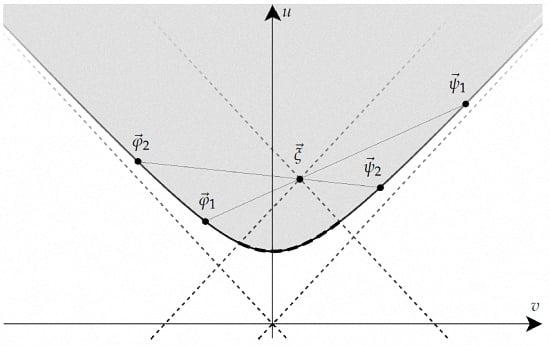
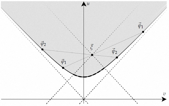
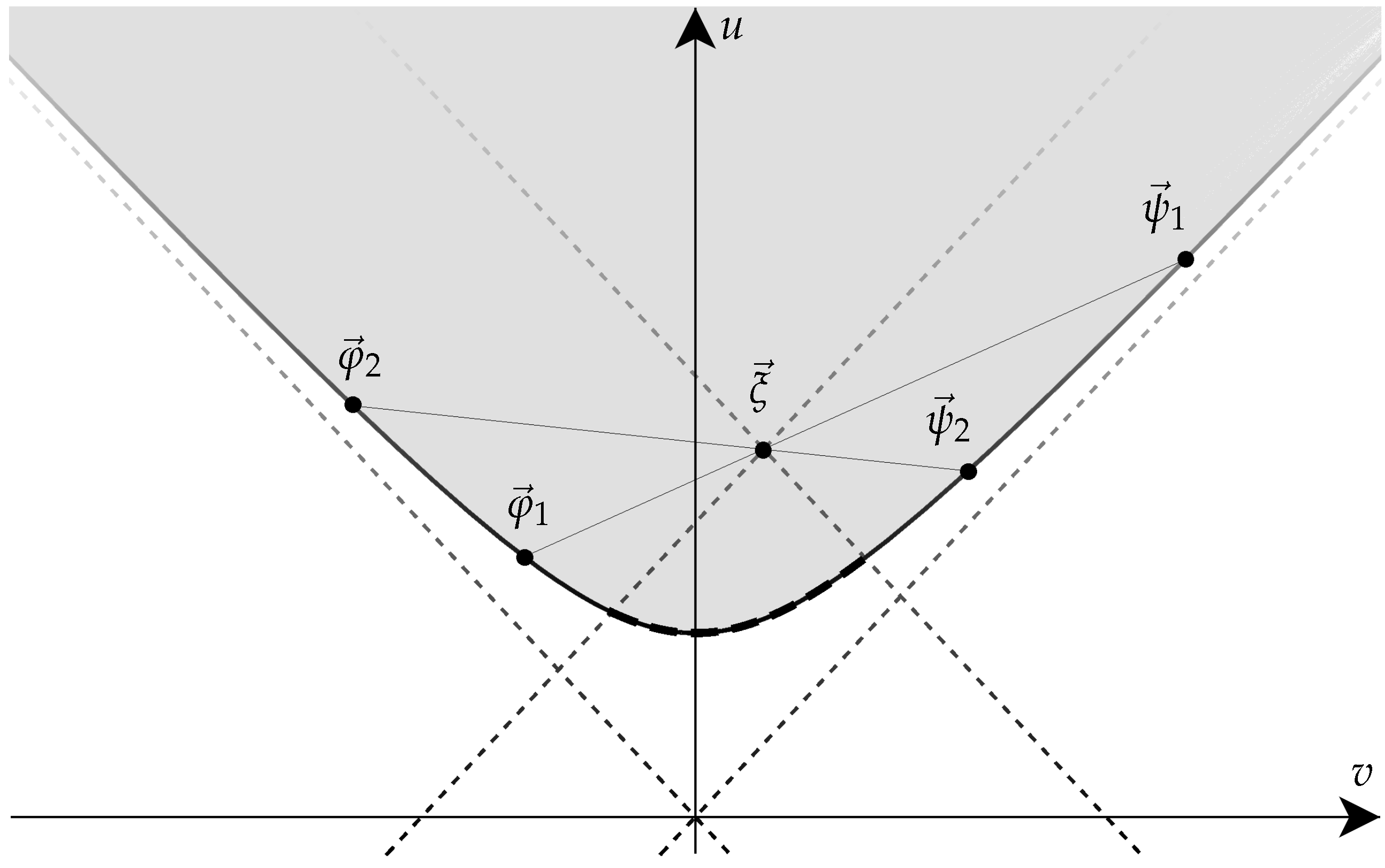
4.1.1. The Uncertainty Region Has a Convex Boundary

The region defined by Equation (29) is a convex set in the N ( 2 N + 1 ) -dimensional space of second moments. To see this, we consider two covariance matrices C 1 and C 2 that are located on its boundary given by (64), i.e., they satisfy
det C 1 = det C 2 = 2 2 N
We recall that covariance matrices are positive definite, C 1 , C 2 > 0 , and that they must have sufficiently large symplectic eigenvalues in order to stem from quantum states. Convexity holds if the (positive definite) convex combination of two covariance matrices,
C ( t ) = t C 1 + ( 1 t ) C 2 , t [ 0 , 1 ]
either lies on the boundary of the uncertainty region or in its interior. This property follows from the fact that the matrix function
g ( A ) = ln det A
is convex [27], i.e., the inequality
g ( t A + ( 1 t ) A ) t g ( A ) + ( 1 t ) g ( A )
holds for any pair of strictly positive definite matrices, A , A > 0 . Rewriting (65) in the form
ln det C 1 / = ln det C 2 / = 2 N ln 2
one immediately finds that
ln det t C 1 + ( 1 t ) C 2 / t ln det C 1 / ( 1 t ) ln det C 2 / = 2 N ln 2
Since
det t C 1 + ( 1 t ) C 2 2 2 N , t [ 0 , 1 ]
follows, and we have shown that the convex combination of two covariance matrices on the boundary of the uncertainty region cannot produce a point outside of it. Equality holds in (71) only if t = 0 or t = 1 . Therefore, states on the boundary cannot be written as mixtures, which means that the states on the boundary must be pure states.
Clearly, the argument just given extends to convex combinations of covariance matrices located inside the uncertainty region: no such combination will produce a covariance matrix on its boundary or outside of it.

4.1.2. The Uncertainty Region Has No Pure-State Holes

We determined the conditions for uncertainty functionals to have extrema by evaluating them on all pure states of N quantum particles. We now show that the inclusion of mixed states as potential extrema does not change our findings. It is sufficient to show that all points of the uncertainty region defined by the inequality (29) correspond to covariance matrices that stem from pure states.
Recall that any admissible covariance matrix can be diagonalised according to Williamson’s theorem [21,23] using a suitable symplectic transformation. Let us order its N finite symplectic eigenvalues s 1 to s N from smallest to largest and choose an integer M 2 such that s N M + 1 2 holds. Suppose now that the k-th subsystem resides in the pure state
| ψ k = t k | n k = 0 + 1 t k | n k = M , k { 1 , , N } , t k [ 0 , 1 ]
The variances of position and momentum take the values
Δ 2 p k ψ k = Δ 2 q k ψ k = ( 1 t k ) M + 1 2 , k { 1 , , N } , t k [ 0 , 1 ]
where we use the fact that the expectations of the operators p ^ k and q ^ k vanish (cf. remark after Equation (3)). Thus, a suitable value of the parameter t k leads to the desired entries s k on the diagonal of the covariance matrix, and the covariance of position and momentum p ^ k and q ^ k equals zero. In addition, the remaining off-diagonal matrix elements—associated with the bilinear operators p ^ k q ^ k for k k —also vanish in the product state
| Ψ = | ψ 1 | ψ N
Consequently, there is a pure product state, namely | Ψ , to generate any desired diagonal covariance matrix—which is sufficient to create any admissible non-diagonal covariance matrix, simply by undoing the symplectic transformation used to diagonalize the initially given covariance matrix.
The map from the set of pure states to the interior of the space of moments is, of course, many-to-one. This can be seen directly by recalling that each admissible covariance matrix C can also be obtained from a Gaussian state characterized by a quadratic form determined by the matrix C .

4.1.3. All Moments Arise as Convex Combinations of Two Pure States

Given any point inside the uncertainty region, one can find infinitely many convex combinations of two pure Gaussian states on the boundary that produce the desired N ( 2 N + 1 ) moments. Here is one way to construct such pairs. Consider any two-dimensional Euclidean plane that passes through the origin of the space of moments, R N ( 2 N + 1 ) , and the given point inside the uncertainty region. The intersection of its boundary with the plane is a one-dimensional set of points that divides the plane into two regions corresponding to acceptable covariance matrices (forming the uncertainty region) and the rest. This line inherits convexity from the boundary in the space S since any two points on the curve are, of course, also located on the high-dimensional boundary.
To conclude the argument, we only need to identify two points on the boundary such that the line connecting them goes through the point representing the desired set of moments. It is geometrically obvious that there exist infinitely many pairs of points on the boundary that satisfy this requirement. This situation is illustrated in Figure 1 in Section 4.2.3 for a single continuous variable where the boundary of the uncertainty region is known to be a hyperbola.

4.2. One Continuous Variable: N = 1

It is instructive to study the properties of the uncertainty region for a single continuous variable since the space of moments has only three dimensions. Even in the absence of entangled states, the uncertainty region has a number of interesting features as it resembles the Bloch ball used to visualize the states of a qubit. For one continuous variable, each point inside the uncertainty region is characterized uniquely by a triple of numbers, the states on the convex boundary are the only pure states, and the decomposition of mixed states into pairs of pure states is clearly not unique. The group of Sp ( 2 , R ) SO ( 2 , 1 ) transformations that leave the uncertainty region invariant play the role of the SU ( 2 ) transformations mapping the Bloch ball to itself.
We simplify the notation to discuss the case N = 1 . Renaming the elements of the 2 × 2 covariance matrix according to
C = Δ 2 p C p q C p q Δ 2 q x w w y
the consistency conditions (34) take the form
x f x = y f y , x f w = 2 w f y
and
x y w 2 = n + 1 2 2 2 , n N 0
The third constraint is universal since it does not depend on the function f ( x , y , w ) that characterizes an uncertainty functional J [ ψ ] . It will be convenient to use the variables
u = 1 2 x + y > 0 , v = 1 2 x y R
to parametrize the points in the three-dimensional space of second moments, with coordinates ( u , v , w ) R 3 . For each non-negative integer, the third condition
u 2 v 2 w 2 = e n 2 , e n = n + 1 2 , n N 0
determines one sheet of a two-sheeted hyperboloid, located in the “upper” half of the space of moments, i.e., u > 0 and v , w R . The n-th sheet—which we call E n , n N 0 —intersects the u-axis at u = + e n , and it is in one-to-one correspondence with the squeezed states originating from the number state | n (cf. [13]).
The states which satisfy Equation (79) for n = 0 saturate the standard Robertson-Schrödinger inequality. Consequently, not all points in the space of moments can arise as moment triples. The accessible part of the space is bounded by the hyperboloid E 0 defined in Equation (79), suggesting us to visualize the uncertainty region as a solid body with boundary E 0 .
We follow the presentation of the multidimensional case in Section 4.1, giving at times alternative proofs of the general results, by appealing to intuition available in the space of second moments due to its low dimension.

4.2.1. The Uncertainty Region Has a Convex Boundary

Given two mixed quantum states described by density matrices ρ ^ 1 and ρ ^ 2 , their convex combinations ρ ^ t = t ρ ^ 1 + ( 1 t ) ρ ^ 2 , t [ 0 , 1 ] , are also quantum states. We now show that the uncertainty region in the space R 3 inherits convexity from the body of density matrices: any convex combination of the states ρ ^ 1 and ρ ^ 2 with moment triples μ k = ( x k , y k , w k ) , k = 1 , 2 , inside the uncertainty region produces another state with a moment triple also in that region. The boundary of an analogously defined uncertainty region for a quantum spin s [28] is not convex. This approach does not use the convexity of the logarithm of positive definite matrices in (68).
The moments x k = Tr ( x ^ 2 ρ ^ k ) , k = 1 , 2 , etc., satisfy the Robertson-Schrödinger inequality,
x k y k w k 2 2 4 e 0 2 , k = 1 , 2
and the moments of the mixture are given by
σ t = t σ 1 + ( 1 t ) σ 2 , σ = x , y , w
Writing t ¯ = 1 t , the variances of the convex combination satisfy
x t y t w t 2 t 2 + t ¯ 2 e 0 2 + t t ¯ x 1 y 2 + x 2 y 1 2 w 1 w 2
using (80). Since
x 1 y 2 + x 2 y 1 2 w 1 w 2 e 0 2 y 2 y 1 + y 1 y 2 + w 1 y 2 y 1 w 2 y 1 y 2 2 2 e 0 2
holds, the moment triple of the convex combination ρ ^ t must also be contained in the uncertainty region, i.e.,
x t y t w t 2 2 4
The minimum is obtained only if either t = 0 or t = 1 , so that the resulting density matrix must describe a state on the boundary of the uncertainty region, i.e., a Gaussian state with minimal uncertainty.

4.2.2. The Uncertainty Region Has No Pure-State Holes

Each mixed state ρ ^ generates a moment triple μ with components x = Tr ρ ^ x ^ 2 , etc., satisfying the Robertson-Schrödinger inequality [29]. Thus, the uncertainty region necessarily contains all potential mixed-state minima μ of a given functional. We want to show that all moment triples inside the uncertainty region can be obtained through pure states. Two cases occur.
If the triple μ is located on one of the hyperboloids E n , n N 0 , then there exists a squeezed number state—i.e., a pure state—which gives rise to the same three expectations. Hence, the point μ has already been included in the search for extrema.
Alternatively, the point μ is located between two hyperboloids, E n and E n + 1 , say, with n N 0 . Again, there is a pure state with moments given by μ . To see this, we first consider only the line segment with end points ( u n , 0 , 0 ) and ( u n + 1 , 0 , 0 ) , which are associated with the number states | n and | n + 1 , respectively. The moments of the superposition
| n t = t | n + 1 t | n + 1 , t [ 0 , 1 ]
indeed lead to all moment triples located on the line segment,
n t = u n + 1 + t u n u n + 1 , 0 , 0 , t [ 0 , 1 ]
since the matrix elements of the second moments between states of different parity vanish.
Finally, any moment triple μ off the u-axis will lie on a hyperboloid with a specific value of t = t 0 , for example. This moment triple can be obtained, however, from the state S ^ ( ξ ) | n t 0 , with a suitable value ξ. Using relativistic terminology, the operator S ^ ( ξ ) must induce a Lorentz transformation that maps the given point on the u-axis to the desired point μ on the same hyperboloid.
In conclusion, each triple μ of the uncertainty region can be obtained from a suitable pure state. Thus, mixed states do not give rise to candidates for minima different from those associated with pure states.

4.2.3. All Moments Arise as Convex Combinations of Two Pure States

Consider a state | ξ giving rise to the moment vector ξ = ( u ξ , v ξ , w ξ ) inside the uncertainty region. It is possible to identify infinitely many pairs of Gaussian states on the boundary such that their mixture reproduces the given triple ξ .
On the level of moments, it is geometrically obvious that any moment triple ξ can be reached as a convex combination of two points located on the boundary (cf. Figure 1). It is sufficient to consider states with vanishing covariance, w = 0 . This choice is equivalent to selecting a particular two-dimensional plane in the space of moments that passes through the origin and the given moment triple ξ (cf. Section 4.1). Picking any point φ “space-like” relative to ξ and located on the hyperboloid, the pair determines a line intersecting the boundary in a unique point ψ . Then, the desired point ξ must lie on the line segment ξ ( t ) = φ + t ( ψ φ ) , t [ 0 , 1 ] , connecting the points φ and ψ ; it will pass through the point ξ if
t 0 = u ξ u φ u ψ u φ v ξ v φ v ψ v φ [ 0 , 1 ]
When writing the line segment in the form ξ ( t ) = t ψ + ( 1 t ) φ , it becomes obvious that the reasoning valid in the space of moments extends to quantum states. In other words, the mixture
ρ ^ t 0 = t 0 P ^ ψ + ( 1 t 0 ) P ^ φ
of the rank-1 projectors P ^ ψ = | ψ ψ | and P ^ φ = | φ φ | onto Gaussian states on the boundary defines a mixed quantum state with the desired moment triple ξ . Clearly, continuously many other convex combinations of pure states exist that lead to the same moment triple.
The relationships between quantum states and points inside the uncertainty region is, of course, many-to-one. For example, the state | 1 with moment vector ξ 1 = ( 9 2 / 4 , 0 , 0 ) , i.e., the first excited state of a harmonic oscillator with unit mass and frequency, being a pure state, cannot be written as a mixture of two Gaussian states. Nevertheless, suitable mixtures of Gaussian states will produce its moment vector ξ 1 . The only moment vectors ξ that cannot be obtained from mixtures are those on the boundary of the uncertainty region. Here, the relationship between states and moment vectors is one-to-one, in agreement with the fact that these Gaussian states are determined uniquely by their covariance matrix C .

5. Conclusions

We have presented a method to systematically determine lower bounds of uncertainty functionals, defined in terms of second moments of quantum systems with two or more continuous variables. In analogy to the one-dimensional case discussed in [13], we find that the states which extremize an uncertainty functional of N degrees of freedom must satisfy a (non-standard) eigenvalue equation that is quadratic in the 2 N position and momentum operators. If the quadratic form associated with this operator is positive (or negative) definite, Williamson’s theorem ensures that it can be diagonalised by a symplectic transformation. In general, the matrix describing the quadratic form depends on the unknown state suggesting to solve it in a self-consistent way. The solutions of the resulting consistency conditions determine the set of states that minimise a given functional. We also introduced the N ( 2 N + 1 ) -dimensional uncertainty region for a system with N continuous variables. We show that this region is a convex subset of the space of second moments, and the points located on the boundary correspond to Gaussian states with minimal uncertainty.
Applying this method to specific functionals associated with quantum systems described by two continuous variables, we both re-derived existing uncertainty relations and previously unknown ones. We are not aware of other methods to obtain these inequalities.
One of the new inequalities generalizes an existing inequality that is capable of detecting entanglement in states of bi-partite particle systems. This example hints at the possibility to systematically construct inequalities that can be used for entanglement detection: take an arbitrary number of EPR-type operators that pairwise commute, and define a monotonically increasing function of their variances that is finite at the origin. Typically, the lower bound given by the value of the functional at the origin will be achieved by an entangled state, and it will be smaller than the value of the functional, which it can take in any separable state. This bound can be obtained by solving the consistency conditions (39) for product states as described in Section 3.1. Clearly, a violation of the pure-state bound will detect the presence of an entangled state. The details of this construction will be left to a future publication.

Acknowledgments

S.K. has been supported via the act “Scholarship Programme of the State Scholarship Foundation (IKY) by the procedure of individual assessment, of 2011–2012” by resource of the Operational Programme for Education and Lifelong Learning of the ESF and of the NSF, 2007–2013, as well as by the WW Smith Fund.

Author Contributions

The authors contributed equally to this work.

Conflicts of Interest

The authors declare no conflict of interest.

References

  1. Heisenberg, W. Über den anschaulichen Inhalt der quantentheoretischen Kinematik und Mechanik. Z. Phys. 1927, 43, 172–198. [Google Scholar]
  2. Kennard, E.H. Zur Quantenmechanik einfacher Bewegungstypen. Z. Phys. 1927, 44, 326–352. [Google Scholar] [CrossRef]
  3. Weyl, H. The Theory of Groups and Quantum Mechanics; Robertson, H.P., Ed.; Dover: New York, NY, USA, 1931. [Google Scholar]
  4. Robertson, H.P. The Uncertainty Principle. Phys. Rev. 1929, 34, 163–164. [Google Scholar] [CrossRef]
  5. Schrödinger, E. Zum Heisenbergschen Unschäfeprinzip. Sitzungsber. Preuss. Akad. Wiss. Phys.-Math. Klasse 1930, 19, 296–323. [Google Scholar]
  6. Arthurs, E.; Kelly, J.L. On the Simultaneous Measurement of a Pair of Conjugate Observables. Bell Syst. Tech. J. 1965, 44, 725–729. [Google Scholar] [CrossRef]
  7. Busch, P.; Lahti, P.; Werner, R.F. Proof of Heisenberg’s error-disturbance relation. Phys. Rev. Lett. 2013, 111, 160405. [Google Scholar] [CrossRef] [PubMed]
  8. Ozawa, M. Universally valid reformulation of the Heisenberg uncertainty principle on noise and disturbance in measurement. Phys. Rev. A 2003, 67, 042105. [Google Scholar] [CrossRef]
  9. Bennett, C.H.; Brassard, G. Qyantum cryptography: Public key distribution and coin tossing. In Proceedings of IEEE International Conference on Computers, Systems and Signal Processing, Bangalore, India, 10–12 December 1984; pp. 175–179.
  10. Duan, L.-M.; Giedke, G.; Cirac, J.I.; Zoller, P. Inseparability Criterion for Continuous Variable Systems. Phys. Rev. Lett. 2000, 84, 2722–2725. [Google Scholar] [CrossRef] [PubMed]
  11. Simon, R. Peres-Horodecki Separability Criterion for Continuous Variable Systems. Phys. Rev. Lett. 2000, 84, 2726–2729. [Google Scholar] [CrossRef] [PubMed]
  12. Jackiw, R. Minimum Uncertainty Product, Number-Phase Uncertainty Product, and Coherent States. J. Math. Phys. 1968, 9, 339–346. [Google Scholar] [CrossRef]
  13. Kechrimparis, S.; Weigert, S. Universality in Uncertainty Relations for a Quantum Particle. J. Phys. A 2016. in print. [Google Scholar]
  14. Tasca, D.S.; Walborn, S.P.; Ribeiro, P.H.S.; Toscano, F. Detection of transverse entanglement in phase space. Phys. Rev. A 2008, 78, 010304R. [Google Scholar] [CrossRef]
  15. Toscano, F.; Saboia, A.; Avelar, A.T.; Walborn, S.P. Systematic construction of genuine-multipartite- entanglement criteria in continuous-variable systems using uncertainty relations. Phys. Rev. A 2015, 92, 052316. [Google Scholar] [CrossRef]
  16. Paul, E.C.; Tasca, D.S.; Rudnicki, Ł.; Walborn, S.P. Detecting entanglement of continuous variables with three mutually unbiased bases. Phys. Rev. A 2016, 94, 012303. [Google Scholar] [CrossRef]
  17. Busch, P.; Schönbeck, T.P.; Schroeck, F., Jr. Quantum observables: Compatibility versus commutativity and maximal information. J. Math. Phys. 1987, 28, 2866–2872. [Google Scholar] [CrossRef]
  18. Bialynicki-Birula, I.; Bialynicka-Birula, Z. Uncertainty Relation for Photons. Phys. Rev. Lett. 2012, 108, 140401. [Google Scholar] [CrossRef] [PubMed]
  19. Rudnicki, Ł. Heisenberg uncertainty relation for position and momentum beyond central potentials. Phys. Rev. A 2012, 85, 022112. [Google Scholar] [CrossRef]
  20. Weigert, S. Landscape of uncertainty in Hilbert space for one-particle states. Phys. Rev. A 1996, 53, 2084–2088. [Google Scholar] [CrossRef] [PubMed]
  21. Williamson, J. On the Algebraic Problem Concerning the Normal Forms of Linear Dynamical Systems. Am. J. Math. 1936, 58, 141–163. [Google Scholar] [CrossRef]
  22. Simon, R.; Mukunda, N.; Dutta, B. Quantum-noise matrix for multimode systems: U(n) invariance, squeezing, and normal forms. Phys. Rev. A 1994, 49, 1567–1583. [Google Scholar] [CrossRef] [PubMed]
  23. Arvind; Dutta, B.; Mukunda, N.; Simon, R. The real symplectic groups in quantum mechanics and optics. Pramana 1995, 45, 471–497. [Google Scholar] [CrossRef]
  24. Adesso, G.; Ragy, S.; Lee, A.R. Continuous Variable Quantum Information: Gaussian States and Beyond. Open Syst. Inf. Dyn. 2014, 21, 1440001. [Google Scholar] [CrossRef]
  25. Robertson, H.P. An Indeterminacy Relation for Several Observables and Its Classical Interpretation. Phys. Rev. 1934, 46, 794–801. [Google Scholar] [CrossRef]
  26. Weedbrook, C.; Pirandola, S.; Garcia-Patron, R.; Cerf, N.J.; Ralph, T.C.; Shapiro, J.H.; Lloyd, S. Gaussian quantum information. Rev. Mod. Phys. 2012, 84, 621–669. [Google Scholar] [CrossRef]
  27. Boyd, S.; Vanderberghe, L. Convex Optimization; Cambridge University Press: Cambridge, UK, 2004; p. 74. [Google Scholar]
  28. Dammeier, L.; Schwonnek, R.; Werner, R.F. Uncertainty relations for angular momentum. New J. Phys. 2015, 17, 093046. [Google Scholar] [CrossRef]
  29. Dodonov, V.V.; Kurmyshev, E.Y.; Man’ko, V.I. Generalized uncertainty relation and correlated coherent states. Phys. Lett. A 1980, 79, 150–152. [Google Scholar] [CrossRef]
Figure 1. Cross-section ( w = 0 ) of the uncertainty region (shaded) illustrating the convexity of its boundary u 2 v 2 w 2 = 2 / 4 ; convex combinations of moment triples located on the hyperboloid (associated with pure Gaussian states with minimal uncertainty) reproduce any given moment vector ξ inside the uncertainty region (the points must be outside of the “back-ward light-cone” of the point ξ , indicated by the dashed segment of the hyperbola).
Mathematics 04 00049 g001

