
Morphisms and Order Ideals of Toric Posets

Abstract
:1. Introduction
- ■
- A set is a toric chain of iff C is a chain of for all . (Proposition 5.3)
- ■
- The edge is in the toric transitive closure of iff is in the transitive closure of for all . (Proposition 5.15)
- ■
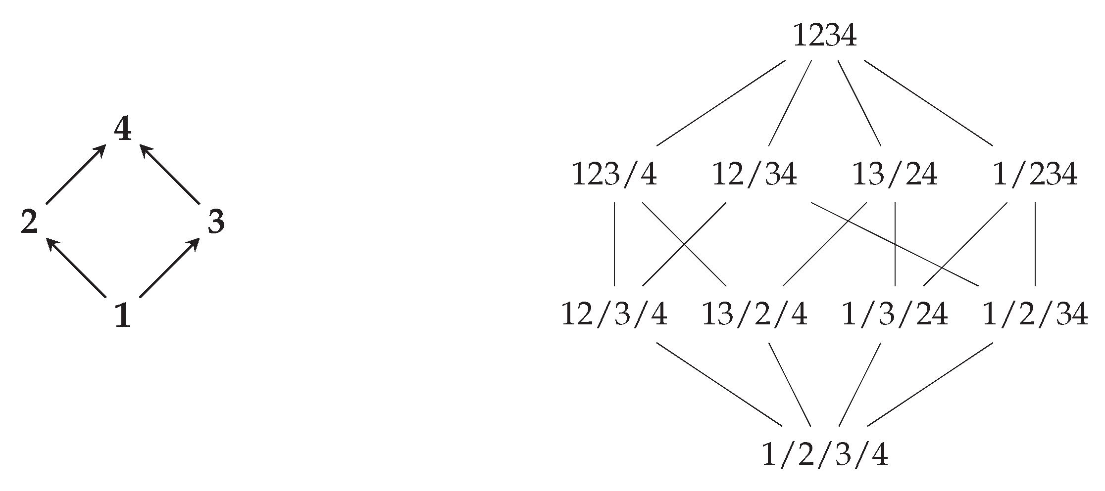
- A partition is a closed toric face partition of iff π is a closed face partition of for some . (Theorem 4.7)
- ■
- A set is a (geometric) toric antichain of iff A is an antichain of for some . (Proposition 5.17)
- ■
- If a set is a toric interval of , then I is an interval of for some . (Proposition 5.14)
- ■
- A set is a toric order ideal of iff J is an order ideal of for some . (Proposition 7.3)
- ■
- Collapsing by a partition is a morphism of toric posets iff collapsing by π is a poset morphism for some . (Corollary 6.2)
- ■
- If an edge is in the Hasse diagram of for some , then it is in the toric Hasse diagram of . (Proposition 5.15)
2. Posets Geometrically
2.1. Posets and Preposets
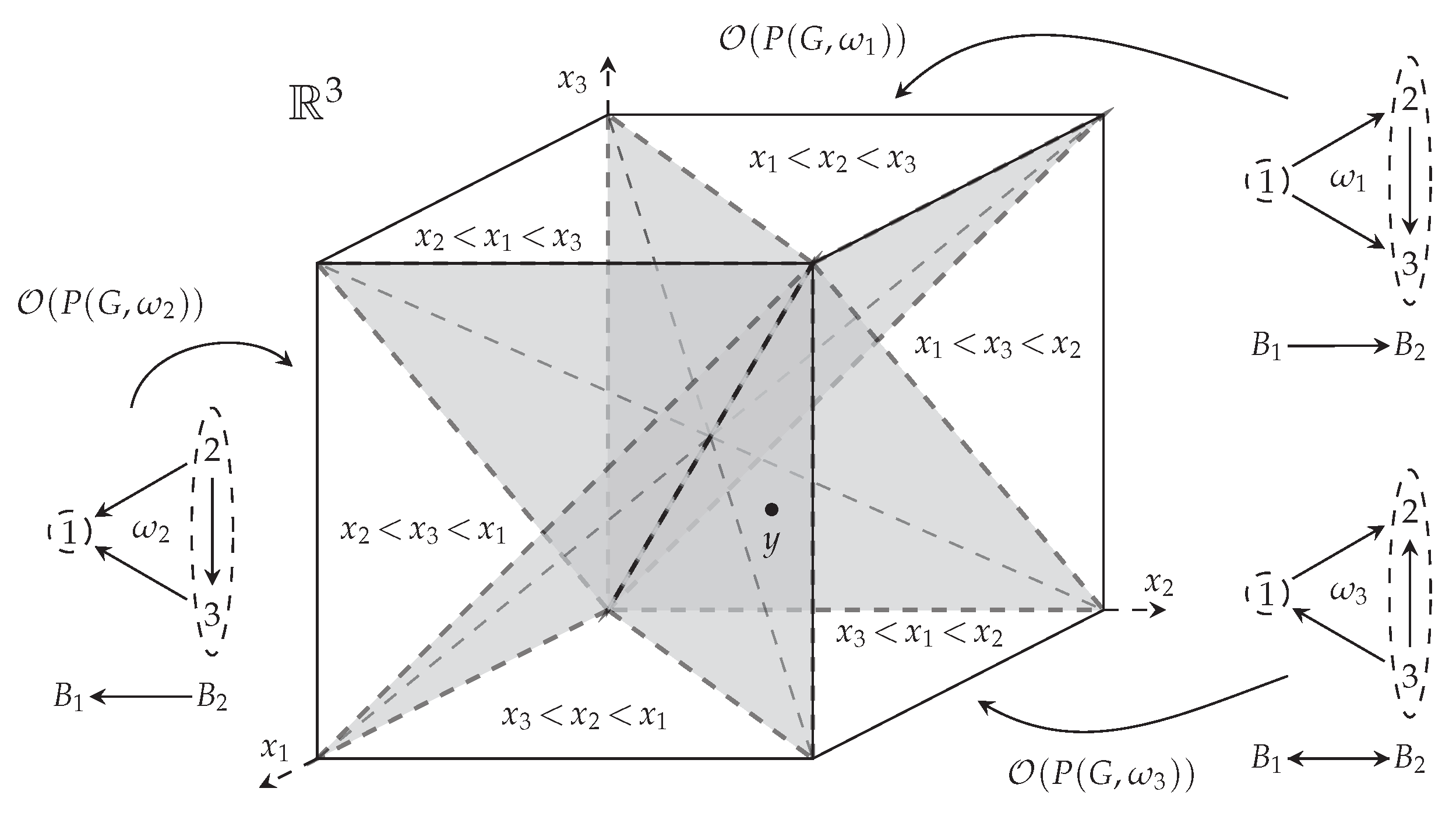
2.2. Chambers of Hyperplane Arrangements

2.3. Face Structure of Chambers
- (i)
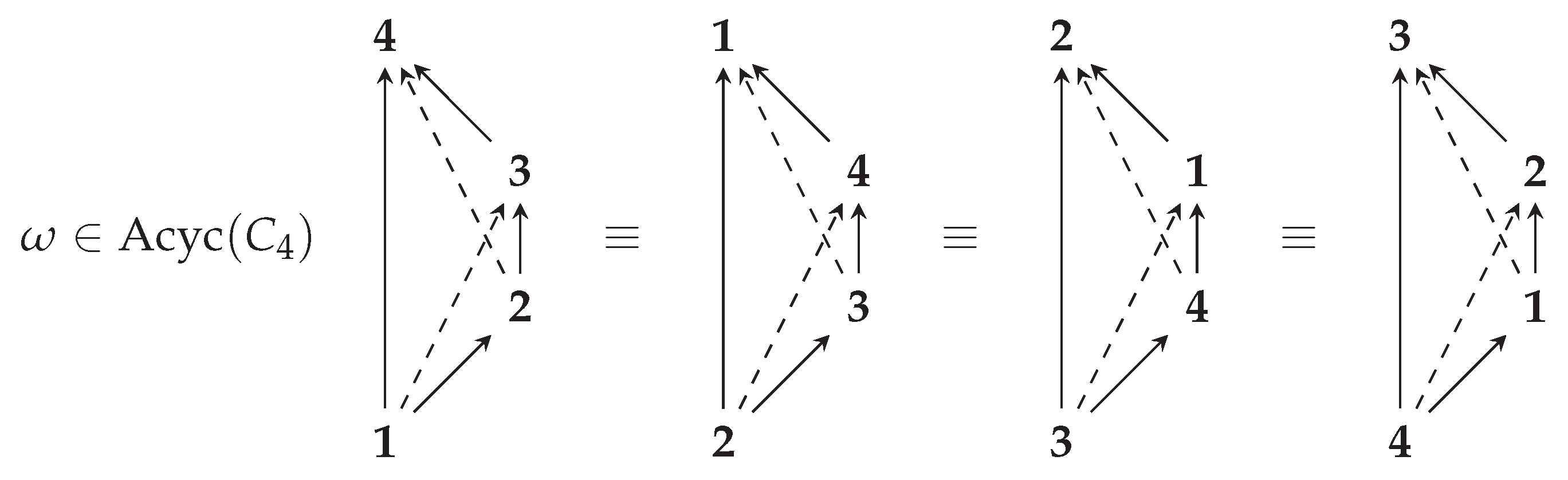
- as a unique orientation of G, where π is the partition into the strongly connected components;
- (ii)
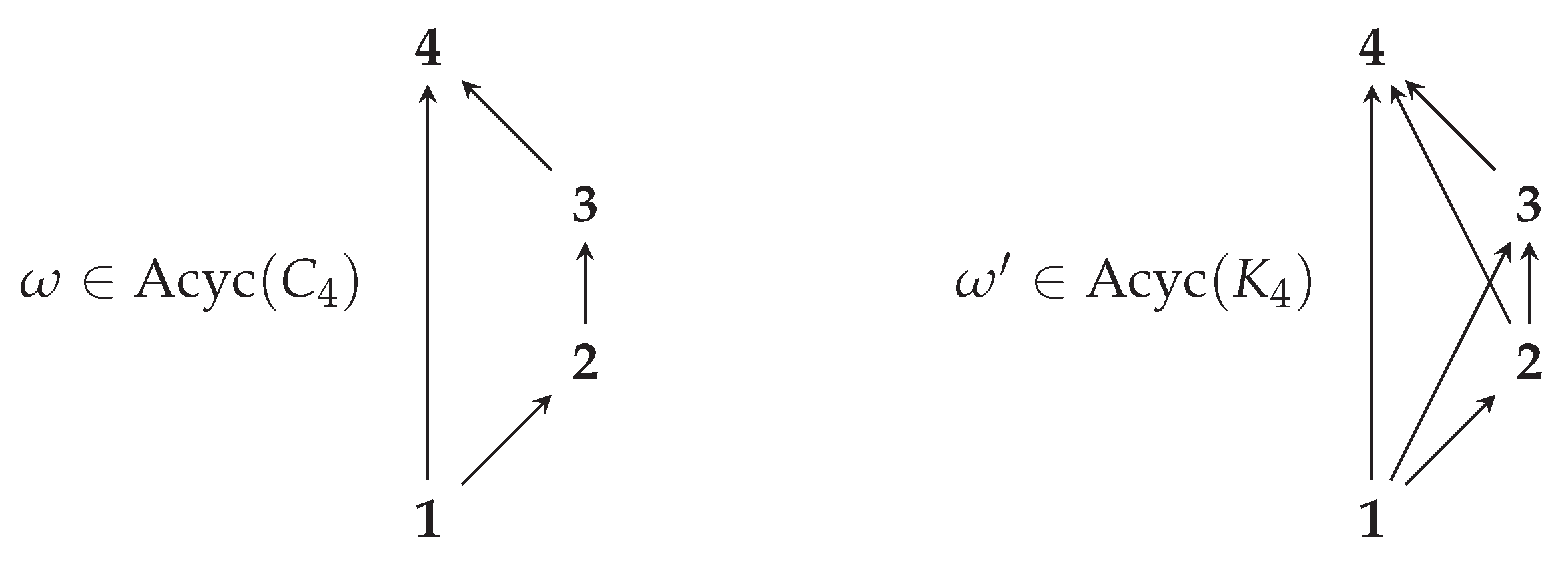
- as a unique acyclic quotient of an acyclic orientation .

3. Morphisms of Ordinary Posets
- combinatorially by the condition that is equivalent to for all ;
- geometrically by the equivalent condition that the induced isomorphism maps to bijectively.
3.1. Quotient
3.1.1. Contracting Partitions


3.1.2. Intervals and Antichains
3.2. Extension
3.3. Inclusion
3.4. Summary
- (i)
- quotient: Collapsing G by a partition π that preserves acyclicity of ω (projecting to a flat of for some closed partition ).
- (ii)
- inclusion: Adding vertices (adding dimensions).
- (iii)
- extension: Adding relations (intersecting with half-spaces).
4. Toric Posets and Preposets
4.1. Toric Chambers and Posets
- ■
- If , then include edge ;
- ■
- If , then include edge .

4.2. Toric Faces and Preposets
- (a)
- If π is closed with respect to , then π is closed with respect to .
- (b)
- Closure is monotone: if , then .
- (c)
- If , then .
- (d)
- .

5. Toric Intervals and Antichains
5.1. Toric Total Orders
5.2. Toric Directed Paths, Chains, and Transitivity
- (a)
- C is a toric chain in P, with .
- (b)
- For every , the set C is a chain of , ordered in some cyclic shift of .
- (c)
- For every , the set C occurs as a subsequence of a toric directed path in , in some cyclic shift of the order .
- (d)
- Every total toric extension in has the same restriction .
5.3. Toric Hasse Diagrams
- (i)
- The edge is in the Hasse diagram, .
- (ii)
- Removing enlarges the chamber .
- (iii)
- is a (closed) facet of P.
- (iv)
- The interval is precisely .
5.4. Toric Intervals
- (i)
- ;
- (ii)
- ;
- (iii)
- .
5.5. Toric Antichains
- combinatorially by the condition that no pair with are comparable, that is, they lie on no common chain of P, or
- geometrically by the equivalent condition that the -dimensional subspace intersects the open polyhedral cone in .
6. Morphisms of Toric Posets
- ■
- quotients that correspond to projecting the toric chamber onto a flat of for some closed toric face partition ;
- ■
- inclusions that correspond to embedding a toric chamber into a higher-dimensional chamber;
- ■
- extensions that add relations (toric hyperplanes).
6.1. Quotient


6.2. Inclusion
6.3. Extension
- ■
- implies ;
- ■
- , where ⊆ is inclusion of edge sets;
- ■
- .
6.4. Summary
- (i)
- quotient: Collapsing G by a partition π that preserves acyclicity of some (projecting to a flat of for some partition ).
- (ii)
- inclusion: Adding vertices (adding dimensions).
- (iii)
- extension: Adding relations (cutting the chamber with toric hyperplanes).
7. Toric Order Ideals and Filters
- ■
- for all in I;
- ■
- for all in J;
- ■
- for all and .
- ■
- for all in I;
- ■
- for all in J.
- (i)
- I is a toric filter of ;
- (ii)
- I is an ideal of for some ;
- (iii)
- I is a filter of for some ;
- (iv)
- In at least one total toric extension of , the elements in I appear in consecutive cyclic order.
8. Application to Coxeter Groups


9. Concluding Remarks
Conflicts of Interest
References
- Eriksson, K. Node firing games on graphs. Contemp. Math. 1994, 178, 117–127. [Google Scholar]
- Eriksson, H.; Eriksson, K. Conjugacy of Coxeter Elements. Electron. J. Combin. 2009, 16, 9. [Google Scholar]
- Shi, J.Y. Conjugacy Relation on Coxeter Elements. Adv. Math. 2001, 161, 1–19. [Google Scholar] [CrossRef]
- Speyer, D. Powers of Coxeter Elements in Infinite Groups are Reduced. Proc. Am. Math. Soc. 2009, 137, 1295–1302. [Google Scholar] [CrossRef]
- Chen, B. Orientations, lattice polytopes, and group arrangements I, Chromatic and tension polynomials of graphs. Ann. Comb. 2010, 13, 425–452. [Google Scholar] [CrossRef]
- Ehrenborg, R.; Slone, M. A geometric approach to acyclic orientations. Order 2009, 26, 283–288. [Google Scholar] [CrossRef]
- Propp, J. Lattice structure for orientations of graphs. 1993. Available online: http://arxiv.org/abs/math/0209005 (accessed on 30 May 2016).
- Marsh, R.; Reineke, M.; Zelevinsky, A. Generalized associahedra via quiver representations. Trans. Am. Math. Soc. 2003, 355, 4171–4186. [Google Scholar] [CrossRef]
- Develin, M.; Macauley, M.; Reiner, V. Toric partial orders. Trans. Am. Math. Soc. 2016, 368, 2263–2287. [Google Scholar] [CrossRef]
- Greene, C. Acyclic orientations. In Higher Combinatorics; Aigner, M., Ed.; D. Reidel: Dordrecht, The Netherlands, 1977; pp. 65–68. [Google Scholar]
- Zaslavsky, T. Orientation of signed graphs. Eur. J. Comb. 1991, 12, 361–375. [Google Scholar] [CrossRef]
- Postnikov, A.; Reiner, V.; Williams, L. Faces of generalized permutohedra. Doc. Math. 2008, 13, 207–273. [Google Scholar]
- Zaslavsky, T. Facing up to Arrangements: Face-Count Formulas for Partitions of Space by Hyperplanes: Face-count Formulas for Partitions of Space by Hyperplanes; American Mathematical Society: Providence, RI, USA, 1975; Volume 154. [Google Scholar]
- Wachs, M. Poset topology: Tools and applications. In Geometric Combinatorics, IAS/Park City Mathematics Series; IAS/Park City Mathematics Institute: Salt Lake City, UT, USA, 2007; pp. 497–615. [Google Scholar]
- Geissinger, L. The face structure of a poset polytope. In Proceedings of the Third Caribbean Conference on Combinatorics and Computing, Cave Hill, Barbados, 5–8 January 1981.
- Stanley, R. Two poset polytopes. Discret. Computat. Geom. 1986, 1, 9–23. [Google Scholar] [CrossRef]
- Backman, S.; Hopkins, S. Fourientations and the Tutte polynomial. 2015. Available online: http://arxiv.org/abs/1503.05885 (accessed on 30 May 2016).
- Christensen, R. Plane Answers to Complex Questions: The Theory of Linear Models; Springer: Berlin, Germany, 2011. [Google Scholar]
- Ward, M. The closure operators of a lattice. Ann. Math. 1942, 43, 191–196. [Google Scholar] [CrossRef]
- Edelman, P.H.; Jamison, R.E. The theory of convex geometries. Geom. Dedicata 1985, 19, 247–270. [Google Scholar] [CrossRef]
- Stanley, R. Enumerative Combinatorics; Cambridge University Press: Cambridge, UK, 2001; Volume 2. [Google Scholar]
- Sturmfels, B. Gröbner Bases and Convex Polytopes; American Mathematical Society: Providence, RI, USA, 1996; Volume 8. [Google Scholar]
- Stembridge, J.R. On the fully commutative elements of Coxeter groups. J. Algebraic Comb. 1996, 5, 353–385. [Google Scholar] [CrossRef]
- Stembridge, J.R. The enumeration of fully commutative elements of Coxeter groups. J. Algebraic Comb. 1998, 7, 291–320. [Google Scholar] [CrossRef]
- Boothby, T.; Burkert, J.; Eichwald, M.; Ernst, D.; Green, R.; Macauley, M. On the cyclically fully commuative elements of Coxeter groups. J. Algebraic Combin. 2012, 36, 123–148. [Google Scholar] [CrossRef]
- Marquis, T. Conjugacy classes and straight elements in Coxeter groups. J. Algebra 2014, 407, 68–80. [Google Scholar] [CrossRef]
- Pétréolle, M. Characterization of cyclically fully commutative elements in finite and affine Coxeter groups. 2014. Available online: http://arxiv.org/abs/1403.1130 (accessed on 30 May 2016).


© 2016 by the author; licensee MDPI, Basel, Switzerland. This article is an open access article distributed under the terms and conditions of the Creative Commons Attribution (CC-BY) license (http://creativecommons.org/licenses/by/4.0/).
Share and Cite
Macauley, M. Morphisms and Order Ideals of Toric Posets. Mathematics 2016, 4, 39. https://doi.org/10.3390/math4020039
Macauley M. Morphisms and Order Ideals of Toric Posets. Mathematics. 2016; 4(2):39. https://doi.org/10.3390/math4020039
Chicago/Turabian StyleMacauley, Matthew. 2016. "Morphisms and Order Ideals of Toric Posets" Mathematics 4, no. 2: 39. https://doi.org/10.3390/math4020039