Counting Rules for Computing the Number of Independent Sets of a Grid Graph

Abstract

The issue of counting independent sets of a graph, G, represented as $i\left(G\right)$, is a significant challenge within combinatorial mathematics. This problem finds practical applications across various fields, including mathematics, computer science, physics, and chemistry. In chemistry, $i\left(G\right)$ is recognized as the Merrifield–Simmons (M-S) index for molecular graphs, which is one of the most relevant topological indices related to the boiling point in chemical compounds. This article introduces an innovative algorithm designed for tallying independent sets within grid-like structures. The proposed algorithm is based on the ‘branch-and-bound’ technique and is applied to compute $i\left(G_{m,n}\right)$ for a square grid formed by m rows and n columns. The proposed approach incorporates the widely recognized vertex reduction rule as the basis for splitting the current subgraph. The methodology involves breaking down the initial grid iteratively until outerplanar graphs are achieved, serving as the ’basic cases’ linked to the leaf nodes of the computation tree or when no neighborhood is incident to a minimum of five rectangular internal faces. The time complexity of the branch-and-bound algorithm speeds up the computation of $i\left(G_{m,n}\right)$ compared to traditional methods, like the transfer matrix method. Furthermore, the scope of the proposed algorithm is more general than the algorithms focused on grids since it could be applied to process general mesh graphs.

1. Introduction

While combinatorics has a rich history of addressing counting problems, complexity theory has yielded fewer results in this line in comparison to decision problems. Currently, there exist a limited number of graph counting problems that can be resolved within polynomial time. The realm of combinatorial mathematics and complexity theory has seen the rise of counting problems as a significant area of investigation. Counting algorithms have proven instrumental in addressing real-world challenges across various disciplines such as mathematics, physics, chemistry, and engineering.

There are several counting problems related to count structures in a grid graph, e.g., perfect matching, spanning trees, k-coloring, Hamiltonian circuits, independent sets, acyclic orientations, and so on. For example, one line of research has been the study of the asymptotic Laplacian-energy-like invariant on square lattices. In [1], the authors show that the asymptotic Laplacian-energy-like invariant $LEL\left(G\right)$ for square lattices G is independent of the three boundary conditions, which are the free, the cylindrical, and the toroidal boundary conditions. Moreover, they present that the Laplacian-energy-like invariant per vertex of lattices is independent of the boundary conditions.

Determining the number of independent sets on a graph, G, represented as $i\left(G\right)$, is acknowledged as a challenging problem, even though specialized algorithms have been developed to efficiently address this issue for certain graph topologies. In the context of challenging counting problems, the calculation of $i\left(G\right)$ for a graph, G, has played a crucial role in delineating the boundary between the counting methods that are efficient and those that are deemed intractable.

The computation of the number of independent sets in mesh structures is applied in various contexts, for example, when a square grid graph, $G_{m,n}$ (representing an initial square grid with m rows and n columns), is considered. For instance, within the realm of statistical physics, determining $i\left(G\right)$ has proven valuable when examining the dynamics of gas particles in a space represented by a grid structure. The calculation of $i\left(G\right)$ has been applied in the “hard square model” as a resource to derive the hard quadratic entropy constant [2]. The “hard square model” is also utilized for enumerating configurations of q particles in the Widow–Rowlinson system, extending to cases where $q>2$  [3,4].

Various researchers have explored the challenge of design methods for counting the number of independent sets on square grid graphs. Notably, researchers such as Calkin [5] and Euler [6] have proposed a matrix-based technique for counting independent sets of a grid, and this method is known as the “transfer matrix method”. This method has been extended to compute $i\left(G\right)$ on mesh structures [7].

However, it is believed that most counting problems related to square grids are intractable, since they rely on the two-dimensional character of the grids as a set of unbounded treewidth. Additionally, the author in [8] considers that counting matchings in square grids, counting Hamiltonian cycles in square grids, and counting Clar sets in fullerene graphs are all hard for the complexity class #$P_1$.

A graph invariant is a function applied to a graph, independent of the vertex labeling. A topological index, on the other hand, is a numerical value linked to either the chemical structure or physical attributes of a molecular graph. In general, a topological index is linked to chemical constitution, aiming to establish connections between chemical structure and diverse physical properties, biological activities, or chemical reactivities. Since the ground breaking contributions of Merrifield and Simmons [9], the connection between the number of independent sets of a graph, G (denoted as $i\left(G\right)$ and representing a chemical compound), and the boiling point of the corresponding compound has been acknowledged. Subsequent to the initial study mentioned earlier, extensive research has been conducted in computational chemistry concerning the calculation of $i\left(G\right)$ while exploring various topologies for molecular graphs.

The branch and bound paradigm is a widely utilized approach for addressing problems characterized by intrinsic combinatorial exponential complexity. This method involves branching the input problem into analogous subproblems with a reduced dimension (size) concerning the original problem. The branching process leads to the formation of an enumerative tree, with leaves representing base cases of the problem that can be solved efficiently. This structured approach facilitates the efficient resolution of those base instances.

Different exponential algorithms have been designed to compute the M-S index on square grids $G_{m,n}$, starting with the super-exponential algorithm based on the transfer matrix method [5,6]. More recently, De Ita et al. [10] propose an exponential-time algorithm based on the use of computing threads for computing $i\left(G_{m,n}\right)$. Meanwhile, in this work, a branch-and-bound algorithm is introduced, whose time complexity is of order $O({\left(1.1939\right)}^{(m-1)\ast (n-1)}\ast poly(m,n))$, where $poly(m,n)$ represents a function with a polynomial-time complexity, and m and n are the dimensions of the grid graph.

Notice that all the above algorithms are of exponential order, and the last two algorithms have a different way of measuring the hard exponential complexity of counting independent sets on square grids, since the algorithm in [10] has an exponential growth based on the number of squares by row (or by columns) in the grid. However, for the algorithm presented here, the exponential growth depends on the number of applications of the ramification vertex rule until achieving basic case subgrids. This algorithmic proposal is more general than the algorithms specifically designed to compute the Merrifield–Simmons index in grid graphs since it can process more general topologies such as polygonal mesh graphs due to the ramification vertex rule, which has a widespread application on all types of graphs.

For example, the proposed algorithm offers an exact solution applicable to grids of various types, including regular grids and those with an irregular number of faces by rows. Notably, the time complexity function obtained in this work for calculating $i\left(G_{m,n}\right)$ exhibits significantly slower growth compared to the complexity function associated with the classical transfer matrix method. This underscores the efficiency and versatility of the proposed algorithm across different grid configurations.

This paper is structured as follows: Section 1 provides a general introduction. Section 2 introduces the preliminaries and the notation that will be employed. In Section 3, the main technique used for designing counting algorithms on grids is presented. Section 4 introduces three counting rules facilitating the processing of various basic cases in the enumerative tree. Section 5 presents the enumerative tree constructed by the proposed algorithm. The final section offers conclusions drawn from this work.

2. Preliminaries

Let $G=(V,E)$ be an undirected simple graph, where V is the set of vertices and E is the set of edges. It is assumed that G does not have loops or parallel edges. The edge connecting the vertices u and v is denoted by $uv$, and sometimes $\{u,v\}$ is used to denote an edge $uv$.

The neighborhood of $x\in V$ is the set $N\left(x\right)=\{y\in V:xy\in E\}$. Meanwhile, $N\left[x\right]=N\left(x\right)\cup \left\{x\right\}$ denotes the closed neighborhood of x. The degree of a vertex x in the graph G, denoted by ${\delta }_G\left(x\right)$, is $\left|N\right(x\left)\right|$. The degree of the graph G is $\mathsf{\Delta }\left(G\right)=max\{{\delta }_G\left(x\right):x\in V\}$. Let $\left|A\right|$ be the cardinality of the set A.

A subset of vertices $S\subseteq V$ in a graph, G, is termed an “independent set” if for every pair of vertices u and v in S, the edge $\{u,v\}$ is not present in $E\left(G\right)$. The notation $I\left(G\right)$ is employed to represent the collection of all independent sets in the graph G.

To specifically denote the independent sets in G containing the vertex v, the notation $I_v\left(G\right)$ is used. Conversely, $I_{-v}\left(G\right)$ represents the independent sets in G where the vertex v is absent.

On the other hand, to denote the number of independent sets in the graph G, the notation $i\left(G\right)$ is used. Specifically, in this context, $i\left(G\right)$ corresponds to the cardinality of the set $I\left(G\right)$. An independent set $S\in I\left(G\right)$ is deemed a “maximal independent set” if it is not a subset of any other independent set within G. Furthermore, if the length of set S is the maximum among all elements in $I\left(G\right)$, then S qualifies as a “maximum independent set” (MIS of G).

The computation of $i\left(G\right)$ is a #P-complete problem for graphs G, where $\mathsf{\Delta }\left(G\right)\ge 3$  [3,11,12,13]. Calculating $i\left(G\right)$ continues #P-complete, even under the constraint of three regular graphs [12]. Nevertheless, for certain graph topologies, G, there exist some polynomial methods to determine $i\left(G\right)$ under the condition that $\mathsf{\Delta }\left(G\right)\le 2$ [14,15,16].

Planar graphs hold significance in both graph theory and the realm of graph drawing. A graph, G, is termed a planar graph when it can be represented as an embedding in the plane. The regions enclosed by the vertices and edges are recognized as the internal faces of the graph. Simultaneously, the unbounded face is identified as the outer face or external face of the graph. An outerplanar graph is defined as a planar graph that can be depicted in a manner where all its vertices are incident to the outer face. In the context of an embedding of a planar graph, G, external vertices as those incident to the outer face are distinguished, while the remaining vertices are considered internal vertices of G.

$F\left(G\right)=\{f_1,\dots ,f_k\}$ denotes the collection of non-intersecting internal faces, or simply faces, of the planar graph G. Every face $f_i\in F\left(G\right)$ is defined by the set of edges that form its boundary and encloses its interior. It is important to note that the outer face of the graph is excluded from the set $F\left(G\right)$. In the context of adjacency among faces in G, two distinct faces are considered adjacent if they share common edges. Conversely, when there are no common edges, the relationship between two faces is described as that of independent faces. Consequently, two independent faces may share common vertices but do not have any edges in common.

A particular type of planar graph is referred to as a grid graph, and it is denoted as $G_{m,n}=(V,E)$ and it is a grid graph of size $mxn$; then, the vertex set is $V=\left\{\right(i,j):1\le i\le m,1\le j\le n\}$, and the edge set is $E=\left\{\right((j,i),(j+1,i)\left)\right|1\le j<m,1\le i\le n\}\cup \{\left(\right(j,i),(j,i+1\left)\right)|1\le j<m,1\le i<n\}$. In this scenario, $G_{m,n}$ denotes a square grid graph with m rows and n columns. And let $k=(m-1)\times (n-1)$, which represents the number of internal faces (tilings) of $G_{m,n}$.

Some studies on structures embedded within a grid graph have been conducted, including Hamiltonian cycles, spanning trees, acyclic orientations, k-coloring, and independent sets [5,6,17,18]. The enumeration of mathematics objects on grids extends to various applications, such as tiling and the development of efficient coding schemes for data storage [19].

A primary approach for counting independent sets on grid graphs $G_{m,n}$ involves the use of the transfer matrix method [5,6]. However, when applied to compute $i\left(G_{m,n}\right)$, this method exhibits a super-exponential time complexity with respect to the dimensions m and n of the grid. Additionally, when extended to more general mesh structures, the resulting algorithms experience a highly exponential increase in complexity over the computation time [7,20].

3. Algorithm Proposal

A branch-and-bound algorithm involves two main phases. The first phase is the branching process, which involves breaking down the graph into two subgraphs through an iterative process, forming an enumeration tree. The second phase is the bound process. This process begins by recognizing that the graph linked with the present node of the enumeration tree acts as a base case for the counting process.

The proposed algorithm for counting independent sets requires a base case graph that is a subgraph of a grid. To qualify as a base case, the subgraph $G_s$ must meet the condition that the closed neighborhood $N\left[v\right]$ of any vertex $v\in V\left(G_s\right)$ is not incident to at least five different internal faces of $G_s$.

It is possible to process any graph associated with a base case in polynomial time with respect to the size of the current graph. The first step in counting the number of independent sets of the graph from a base case is to create a Hamiltonian path (Hp) on the graph. Simultaneously with the execution of the Hamiltonian path, one of the three fundamental rules specifically designed to maintain a partial count on the independent sets is applied. This count is influenced by the vertices and edges already visited during the tour.

In order to explain the counting process on graphs associated with the base cases, the first step is to illustrate how the Hp is performed on the subgraphs that meet the cut-off condition.

One of the most common ways for traversing a graph is to apply a depth-first search (dfs). Let us consider that G has cycles. A depth-first search will be applied over G. $G_0=dfs\left(G\right)$ denotes to the graph resulting from the application of a dfs on G, and let T be the spanning tree formed during the application of the dfs. The edges in T are called tree edges. An edge $e\in \left(E\right(G)-E(TG\left)\right)$ is called a frond edge (or a back edge when it is related to the depth-first search).

Let $e\in \left(E\right(G)-E(TG\left)\right)$ be a frond edge. The union of the path in T between the endpoints of e with the edge e itself forms a simple cycle $C_e$; such a cycle is called a basic cycle of G with respect to T.

The approach involves constructing a Hamiltonian path (Hp) for any subgrid formed by decomposition of the input grid while simultaneously computing the number of independent sets of the graph’s components in an incremental manner. The Hp will visit every vertex only once. Meanwhile, each edge in the subgrid is recognized as a tree edge or a frond edge.

Except for the first and last vertices visited by the Hamiltonian path, the two edges of the vertices of degree 2 are considered tree edges, and they will be processed by the Fibonacci rule. Additionally, for vertices with a degree of 3, two of their edges are traversed as tree edges, while the third edge is identified as a frond edge that is processed by the subtracted rule. On the other hand, the vertices of degree 4 have two of its edges as tree edges, and the remaining two edges are frond edges.

Although the problem of finding a Hamiltonian cycle for any graph is a classic NP-Complete problem [21], in this case, the problem relaxes its constraints by considering paths instead of cycles, which does not force a return to the same starting point of the path. The most significant simplification occurs when considering grid graphs, as the challenge of finding a Hamiltonian path transforms into a problem with linear time complexity. This is because none of the vertices in grid graphs have a degree greater than 4.

For example, the Hp can be constructed using a traversing by columns (or by rows) approach. It is important to ensure that each vertex is visited only once and that each edge is identified as either a tree edge or a frond edge. In a traversing by columns, the direction of the search in the Hp can be from bottom to top for the odd columns and from top to bottom for the even columns. It is common for the last vertex visited in the Hp to have one of its edges as a frond edge.

Two graphical symbols are introduced into a Hamiltonian path of a subgraph of G. The symbol ↦ indicates the beginning of a Hamiltonian path. Meanwhile, the symbol $\to |$ indicates the end of the Hamiltonian path.

4. Counting Rules for Processing Grid Base Cases

Each node $v\in V\left(G\right)$ is associated with a pair $({\alpha }_v,{\beta }_v)$, called the charge of the vertex v, and where ${\alpha }_v=\left|I_{-v}\left(G\right)\right|$ and ${\beta }_v=\left|I_v\left(G\right)\right|$. The charge of a vertex $v\in V\left(G\right)$ will be computed at the time that v is visited during a traversing on G. Thus, the charge of v is an auxiliary temporal pair used for computing the number of independent sets of G and such that if $v_r$ is the last visited vertex during the traversing on G, then $i\left(G\right)={\alpha }_{v_r}+{\beta }_{v_r}$.

There are several methods for computing $i\left(G\right)$ when G belongs to a reduced set of simple graph topologies [14,15,16,22]. In this proposal, the main element is to compute the charge $({\alpha }_v,{\beta }_v)$ for each vertex v in the graph during a Hamiltonian walk on G. Different counting rules could be applied to compute the charge of a vertex v, mainly depending on the topology of the subgraph $N\left[v\right]$, when v is visited during the Hamiltonian walking on G.

Three main counting rules to process any subgrid will be considered.

• Fibonacci rule: used to process tree edges.
• Subtracted rule: applied to process frond edges.
• Product rule: used to converge different search lines.

4.1. The Fibonacci Rule

Let us consider the first simple basic topology of a graph. Let G be a path of size n,and then $G=P_n$. In this case all edges of $P_n$ can be denoted as $e_i=\{i,i+1\},i=1,\dots ,n-1$, where $V\left(P_n\right)=\{1,2,\dots ,n\}$. Let us contemplate the family $f_i=\left\{G_i\right\},i=1,\dots ,n$ where each $G_i=(V_i,E_i)$ represents the induced graph of G created solely from the first i vertices of G.

Notice that $({\alpha }_1,{\beta }_1)=(1,1)$ given that the induced subgraph $G_1=\left\{v_1\right\}$, $I\left(G_1\right)=\{\varnothing ,\left\{v_1\right\}\}$. If the values for $({\alpha }_i,{\beta }_i)$ for any $i<n$ are known, when the subsequent induced subgraph $G_{i+1}$ is constructed from $G_i$ by adding the vertex $v_{i+1}$ and the edge $\{v_i,v_{i+1}\}$, it becomes apparent that the pair $({\alpha }_{i+1},{\beta }_{i+1})$ is derived from $({\alpha }_i,{\beta }_i)$ through the following recurrence relation:

$$\mathbf{Fibonacci}\mathbf{rule}:{\alpha }_{i+1}={\alpha }_i+{\beta }_i;{\beta }_{i+1}={\alpha }_i$$

(1)

The series (${\alpha }_i$,${\beta }_i$), i=1, …,n, built from recurrence (1), leads to $i\left(G_i\right)={\alpha }_i+{\beta }_i$, $i=1,\dots ,n$. Then, the computation of $i\left(G\right)$ relies on the step-by-step calculation of $i\left(G_i\right),i=1,\dots ,n$. The application of recurrence (1) is denoted as → between the pairs $({\alpha }_i,{\beta }_i)$ and $({\alpha }_{i+1},{\beta }_{i+1})$. The application of the previous recurrence will be called a Fibonacci rule recurrence, since when they are applied on a path, $P_n$, the following identity $i\left(P_n\right)={\alpha }_{i+1}+{\beta }_{i+1}=F_{n+1}+F_n=F_{n+2}$ is obtained, where $F_n$ is the $nth-$Fibonacci number.

For example, the computation of $i\left(P_5\right)$ is given as: $(1,1)\to (2,1)\to (3,2)\to (5,3)\to (8,5)$. The series $({\alpha }_i,{\beta }_i),i=1,\dots ,n$ (formed during the computation of $i\left(P_n\right)$) is called a computing thread (or just a thread). Notice that each temporal charge $({\alpha }_i,{\beta }_i)$ can be stored in a structure associated with each vertex $v_i$.

4.2. The Subtracted Rule

Another helpful basic counting rule during a Hamiltonian walk on the grid is applied when visiting a frond edge. In this method, frond edges are processed in two phases. Let $\{v,w\}$ be a frond edge of a graph, G.

In the first phase of this counting rule, when the vertex v of the frond edge is visited, it is necessary to duplicate the number of active threads. Assuming that ${({\alpha }_v,{\beta }_v)}_i$ is the pair associated with the active thread $L_i$ at the time of visiting the vertex v, a new thread $L_{vw\_i}$ is created. This thread is subordinated to the master thread $L_i$ and has an initial associated pair ${(0,{\beta }_v)}_{vw\_i}$. For every active thread $L_i$ where ${\beta }_v>0$, a new thread $L_{vw\_i}$ is created. The label $vw\_i$ from $L_{vw\_i}$ is then used as a pointer to its master thread $L_i$.

The second phase in the processing of the frond edge $\{v,w\}$ occurs when the search visits the vertex w, while v has already been marked as a visited vertex. At this point, the control of the search is kept on the vertex w, which helps avoid visiting any vertex of the graph more than once.

Given the charges ${({\alpha }_w,{\beta }_w)}_i$ and ${({\alpha }_{vw},{\beta }_{vw})}_{vw\_i}$ for the vertex w in the master thread $L_i$ and subordinated thread $L_{vw\_i}$, respectively, the subtracted counting rule can be used to update the charge of w in $L_i$.

$$\mathbf{Subtracted}\mathbf{rule}:{({\alpha }_w,{\beta }_w)}_i={({\alpha }_w,{\beta }_w-{\beta }_{vw})}_i$$

(2)

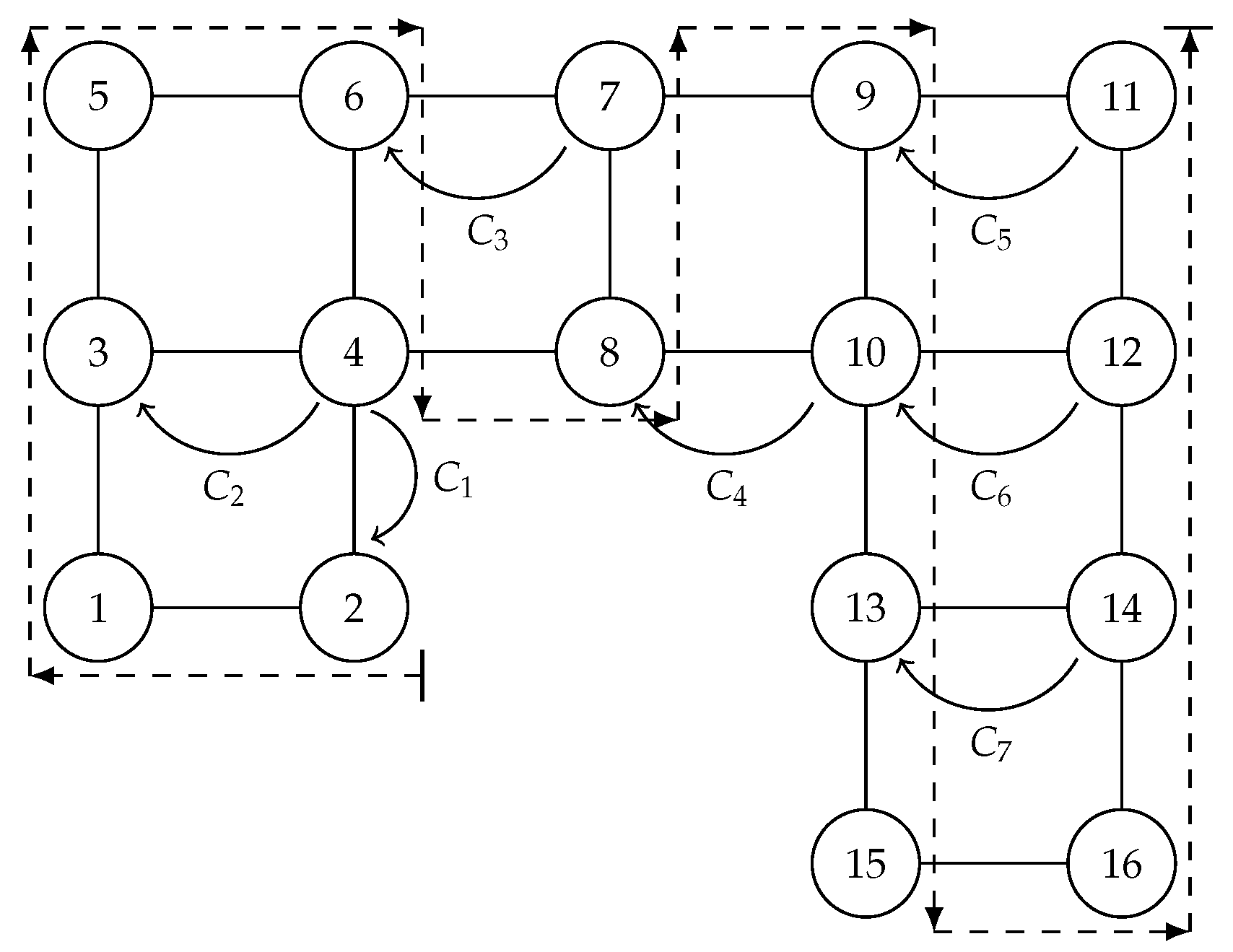
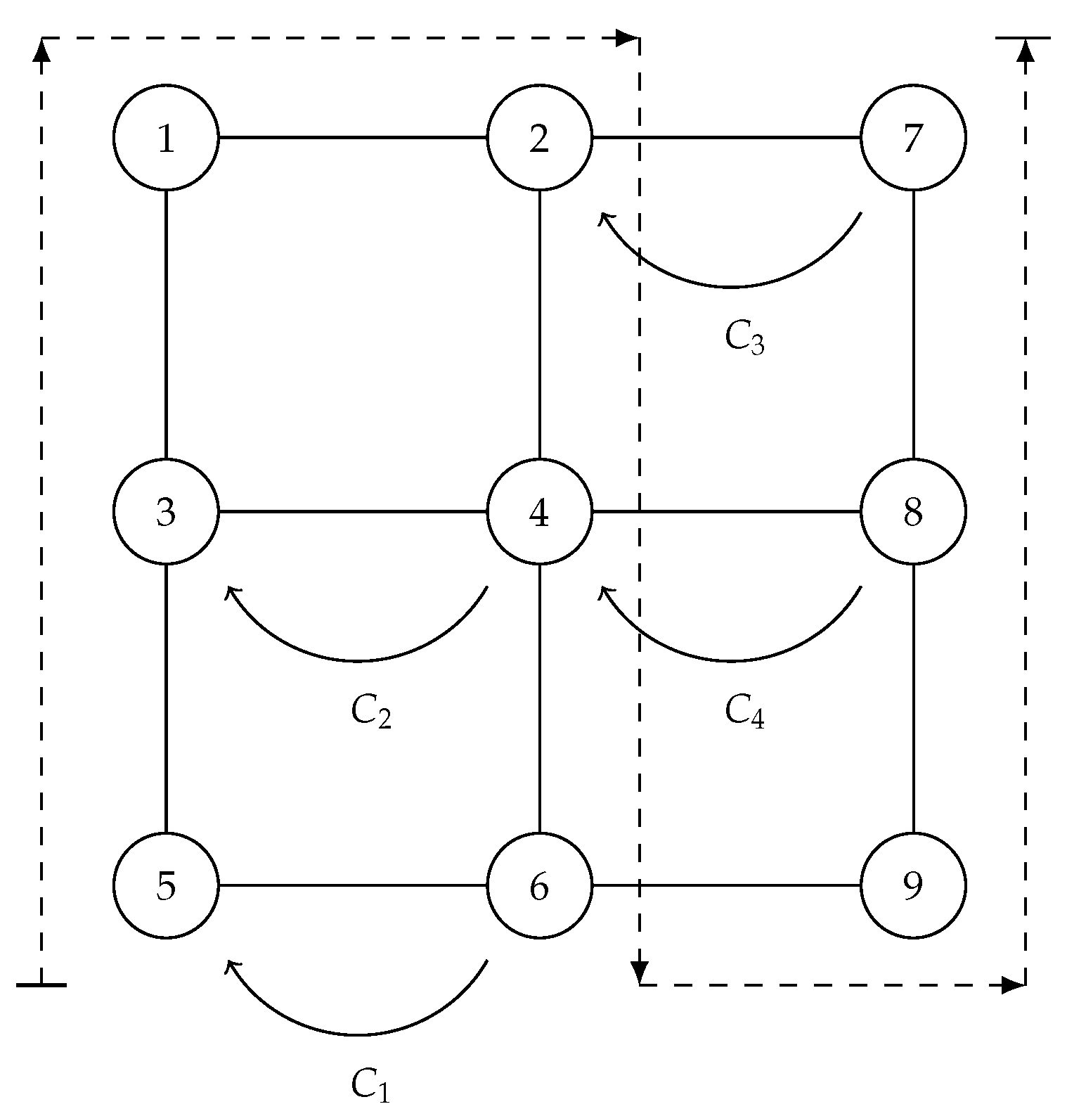
After applying the subtracted rule for the frond edge $\{v,w\}$, all subordinated threads $L_{vw\_i}$ are closed, leading to a decrease in the number of active threads. When illustrating a Hamiltonian path on a subgrid, ⊣ will symbolize the beginning of the path and $\to |$ the end of the path; the processing of a tree edge is symbolized by a dashed line or by $-\to$, and the processing of a frond edge, $vw$, is symbolized by a curved arrow between the vertices v and w. Those previous counting rules are applied while G is traversed by a Hamiltonian path.

Additionally, the Fibonacci and subtracted rules are enough to process any row of tiles in a grid. For example, the following figures illustrate how the Fibonacci and subtracted rules can be applied to process the number of independent sets on subgrids.

In the following tables of the computation of the charges of the vertices of the illustrated graphs, the subindex x after the pair of charges indicates that those computing threads are closed. Meanwhile, the symbol = at the beginning of a charge indicates that the subtracted rule was applied to the two previous pairs.

The order of the Hamiltonian path is presented by the order of the columns in

Table 1. Counting independent sets from Figure 1 (first part).

Vertex 2	1	3	5	6	4$⤺{\mathit{C}}_2{\mathit{C}}_1$	8	7$⤺{\mathit{C}}_3$	9
$L_P$: (1,1)	(2,1)	(3,2)	(5,3)	(8,5)	(13,8) − (0,2) − (0,2) = (13,4)	(17,13)	(30,17) − (0,5) = (30,12)	(42,30)
$C_1$: (0,1)	(1,0)	(1,1)	(2,1)	(3,2)	(5,3) − (0,1) = (5,2)x
	$C_2{L}_p$:	(0,2)	(2,0)	(2,2)	(4,2)x
	$C_2{C}_1$:	(0,1)	(1,0)	(1,1)	(2,1)x
			$C_3{L}_p$:	(0,5)	(5,0)	(5,5)	(10,5)x
			$C_3{C}_1$:	(0,2)	(2,0)x
			$C_3{C}_2{L}_p$:	(0,2)	(2,0)x
			$C_3{C}_2{C}_1$:	(0,1)	(1,0)x
					$C_4{L}_p$:	(0,13)	(13,0)	(13,13)
					$C_4{C}_3{L}_p$:	(0,5)	(5,0)x
							$C_5{L}_p$:	(0,30)
							$C_4{C}_5{L}_p$:	(0,13)

,

Table 2. Counting independent sets from Figure 1 (second part).

10$⤺{\mathit{C}}_4$	13	15	16	14$⤺{\mathit{C}}_7$	12$⤺{\mathit{C}}_6$	11$⤺{\mathit{C}}_5$
$L_P$: (72,42) − (0,13) = (72,29)	(101,72)	(173,101)	(274,173)	(447,274) − (0,72) = (447,202)	(549,447) − (0,87) = (649,360)	(1009,649) − (0,210) = (1009,439)
$C_4{L}_p$: (26,13)x
$C_5{L}_p$: (30,0)	(30,30)	(60,30)	(90,60)	(150,90) − (0,30) = (150,60)	(210,150)	(360,210)x
$C_5{C}_4{L}_p$: (13,0)x
$C_6{L}_P$: (0,29)	(29,0)	(29,29)	(58,29)	(87,58)	(145,87)x
$C_7{L}_P$:	(0,72)	(72,0)	(72,72)	(144,72)x
$C_7{C}_5{L}_P$:	(0,30)	(30,0)	(30,30)	(60,30)x

and

Table 3. Counting independent sets from Figure 2.

Vertex	5	3	1	2	4$⤺{\mathit{C}}_2$	6$⤺{\mathit{C}}_1$	9	8$⤺{\mathit{C}}_4$	7
$L_p$	(1,1)	(2,1)	(3,2)	(5,3)	(8,5) − (0,1)	(12,8) − (5,3)	(17,12)	(29,17) − (0,4)	(42,29) − (0,8)
					=(8,4)	=(12,5)		=(29,13)	=(42,21)
$C_1{L}_P$	(0,1)	(1,0)	(1,1)	(2,1)	(3,2)	(5,3)x
	$C_2{L}_p$	(0,1)	(1,0)	(1,1)	(2,1)x
			$C_3{L}_P$	(0,3)	(3,0)	(3,3) − (0,1)	(5,3)	(8,5)	(13,8)x
						=(3,2)
			$C_3{C}_1{L}_P$	(0,1)	(1,0)	(1,1)x
			$C_3{C}_2{L}_p$	(0,1)	(1,0)x
				$C_4{L}_p$	(0,4)	(4,0)	(4,4)	(8,4)x
				$C_4{C}_1{L}_p$	(0,2)	(2,0)x

. Moreover, each row describes the current charge for the vertex of its corresponding column. The first value in each row is the label describing the name of the corresponding computing thread. The last charge in the row corresponding to $L_p$ will give you the total value for $i\left(G\right)$ for the graphs shown in Figure 1 and Figure 2. For the example in Figure 1, $i\left(G\right)=1009+439=1448$. Meanwhile, for Figure 2, $i\left(G\right)=42+21=63$.

De Ita et al. [10] show how calculating the number of independent sets of a grid is possible by taking the Hamiltonian path as a guide while the two counting rules, the Fibonacci rule and the subtracted rule, are applied. Nevertheless, the time complexity of the aforementioned process is exponentially proportional to the maximum number of frond edges in any row of the grid. This is attributed to the necessity of keeping a substantial number of computing lines active during the processing of open cycles in each row of the grid.

In this proposal, a basic case is a subgrid, $G_G$, where each vertex $v\in G_G$ satisfies the condition that $N\left[v\right]$ is not part of more than five grid faces, and then the computation of $i\left(G_G\right)$ can be performed of polynomial order over the size of $G_G$; this is of order $O\left(poly\right(|G_G\left|\right))$, where poly is a polynomial function.

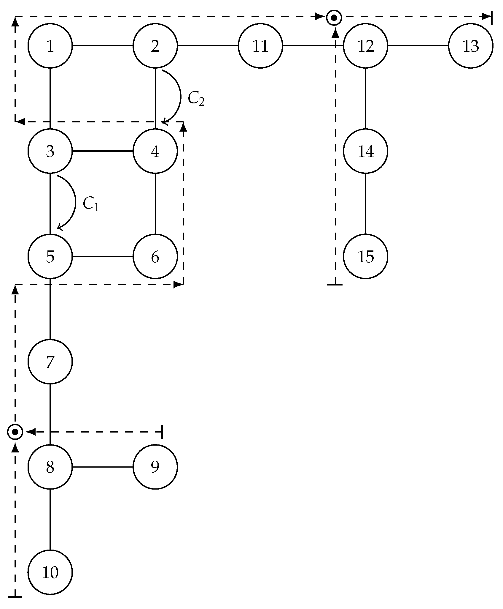
However, the previous rules, the Fibonacci and subtracted rules, are not enough to compute $i\left(G\right)$ when G is a subgrid, as is illustrated in Figure 3. For this case, a new rule called the product rule is introduced.

4.3. The Product Rule

When multiple path searches converge at a meeting vertex, the product rule is used to calculate the interaction between each pair of active threads on one path line and all pairs of active threads on the second path line.

For example, let us consider that there are two computing threads $L_i$ and $L_j$ which have associated the charges $({\alpha }_v,{\beta }_v)$ and $({\alpha }_w,{\beta }_w)$, respectively. Furthermore, the edges $\{v,u\}$ and $\{w,u\}$, with common vertex u, are the next ones to be visited by the Hamiltonian path. In this case, the following multiplicative rule is applied in order to compute the charge for the vertex u.

$$\mathbf{Product}\mathbf{rule}:({\alpha }_u,{\beta }_u)=({\alpha }_v·{\alpha }_w,{\beta }_v·{\beta }_w)$$

(3)

The product rule can be generalized for the Hp that has more than two line searches. Suppose there are child nodes $u_1,u_2,\dots ,u_k$ of v, and all these child nodes have already been visited. In this case, each pair $({\alpha }_{u_j},{\beta }_{u_j})$ for $j=1,...,k$ associated with these child nodes have been previously explored. Therefore, each pair has been established using recurrence (Equation (1)). Then, the charge for v can be computed as: ${\alpha }_v={\prod }_{j=1}^k{\alpha }_{v_j}$ and ${\beta }_v={\prod }_{j=1}^k{\beta }_{v_j}$. The symbol ⊙ will be used to denote when a product rule is applied on the active threads.

The Fibonacci, subtracted, and product rules are enough to compute $i\left(G\right)$ for any subgrid that is recognized as an outerplanar graph. Moreover, these rules can also be applied to compute $i\left(G\right)$ for some subgrids G where G is not outerplanar, but it is planar. The product rule is a useful tool that allows us to establish varying starting points for the Hp. This leads to the convergence of some of the search lines at meeting vertices, resulting in the walking reaching a single end point at the end of the Hp.

Let us illustrate how those previous rules are applied to compute $i\left(G\right)$ for the following subgrid G.

Figure 3. Applying the product rule.

Figure 3. Applying the product rule.

In

Table 4. Counting independent sets from Figure 3.

Start	10	8	7	5	6	4
10	(1,1)	(2,1) * (2,1) = (4,1)	(5,4)	(9,5)	(14,9)	(23,14)
9	(1,1)	(2,1)
			$C_1$	(0,5)	(5,0)	(5,5)
					$C_2{L}_P$	(0,14)
					$C_2{C}_1$	(0,5)
Start	3$⤺{\mathit{C}}_{\mathbf{1}}$	1	2$⤺{\mathit{C}}_{\mathbf{2}}$	11	12	13
$L_p$	(37,23) − (0,5) = (37,18)	(55,37)	(92,55) − (0.14) = (92,41)	(133,92)	(225,133) * (3,2) = (675,266)	(941,675)
${\mathit{C}}_1$	(10,5)x
${\mathit{C}}_2{L}_P$	(14,0)	(14,14)	(28,14)x
$C_2{C}_1$	(5,0)x
15			(1,1)	(2,1)	(3,2)

, the order of the Hamiltonian path is determined by the order of the columns. However, it is important to note that this Hp has different start points that are expressed by the number of the vertex in the corresponding row of the table. Additionally, the first value in each row serves as a label that describes the name of the corresponding computing thread. Whenever you see the symbols “–” and “=” in the table, the subtracted rule is applied. On the other hand, when you see the symbols “*” and “=”, this expresses that the product rule is being applied between two charges.

5. Building the Enumerative Tree

Two prevalent rules govern the counting of combinatorial objects on graphs, enabling us to break down the graph either by the selection of a vertex or by the selection of an edge.

• The counting rule based on a vertex—the vertex division: let $v\in V\left(G\right)$,

  $$i\left(G\right)=i(G-v)+i(G-(N\left[v\right]\left)\right)$$
• The counting rule based on an edge—the edge division: let $e=\{x,y\}\in E\left(G\right)$,

  $$i\left(G\right)=i(G-e)-i(G-(N\left[x\right]\cup N\left[y\right]\left)\right)$$

An alternative rule for decomposing the counting of independent sets is to treat each connected component of the graph independently. For example, let us consider that $G_i,i=1,\dots ,k$ are the connected components of G, and then $i\left(G\right)={\prod }_{i=1}^{k}i\left(G_i\right)$. In this case, the overall time complexity for calculating $i\left(G\right)$ is $T\left(i\left(G\right)\right)=max\{T\left(i\left(G_i\right)\right)$, where $G_i$ is a connected component of $G\}$. Thus, it is common to consider the connected components of the graph as its first decomposition.

In this work, a standard branch-and-bound algorithm was developed, denoted as the BB Algorithm 1, for counting the number of independent sets in a grid graph. The BB algorithm constructs a computation tree, and during the branching processes, it focuses on two key aspects: the criteria for selecting a vertex v (when employing the vertex division rule) and a stopping criterion to cease branching at any node within the computation tree. According to the pseudo-code shown, the proposed algorithm can be implemented in any high-level language that allows recursive processes.

Algorithm 1 BB algorithm
Input: $agridgraphG$ Output: $basecasesfromthegridgraphG$  1: procedure $SelectingNode$(G)  2:      $n\leftarrow \left|V\right(G\left)\right|$  3:      for $i\leftarrow 1,n$ do
4:           $x\leftarrow G\left[i\right]$	▹x is a vertex from G
5:           if $\left(N\right[x]incide>=5internal faces)$ then  6:                return x  7:           end if  8:      end for  9:      return 0 10: end procedure 11: procedure $Branching$(G) 12:      $v\leftarrow SelectingNode\left(G\right)$ 13:      if $(v=0)$ then 14:           $ProcessingBase\_Case\left(G\right)$ 15:      else
16:           $Branching(G-v)$	▹ vertex v is removed from G
17:           $Branching(G-N[v\left]\right)$	▹ the neighborhood (N[v]) is removed from G
18:      end if 19: end procedure

The selected vertex v from the current subgraph, chosen for the application of the vertex division rule, meets the following criteria:

• The neighborhood of v has to be incident with at least five internal faces.
• One of the internal faces incident to $N\left[v\right]$ either possesses the maximum size within the current subgraph, or it shares edges with the outer face.

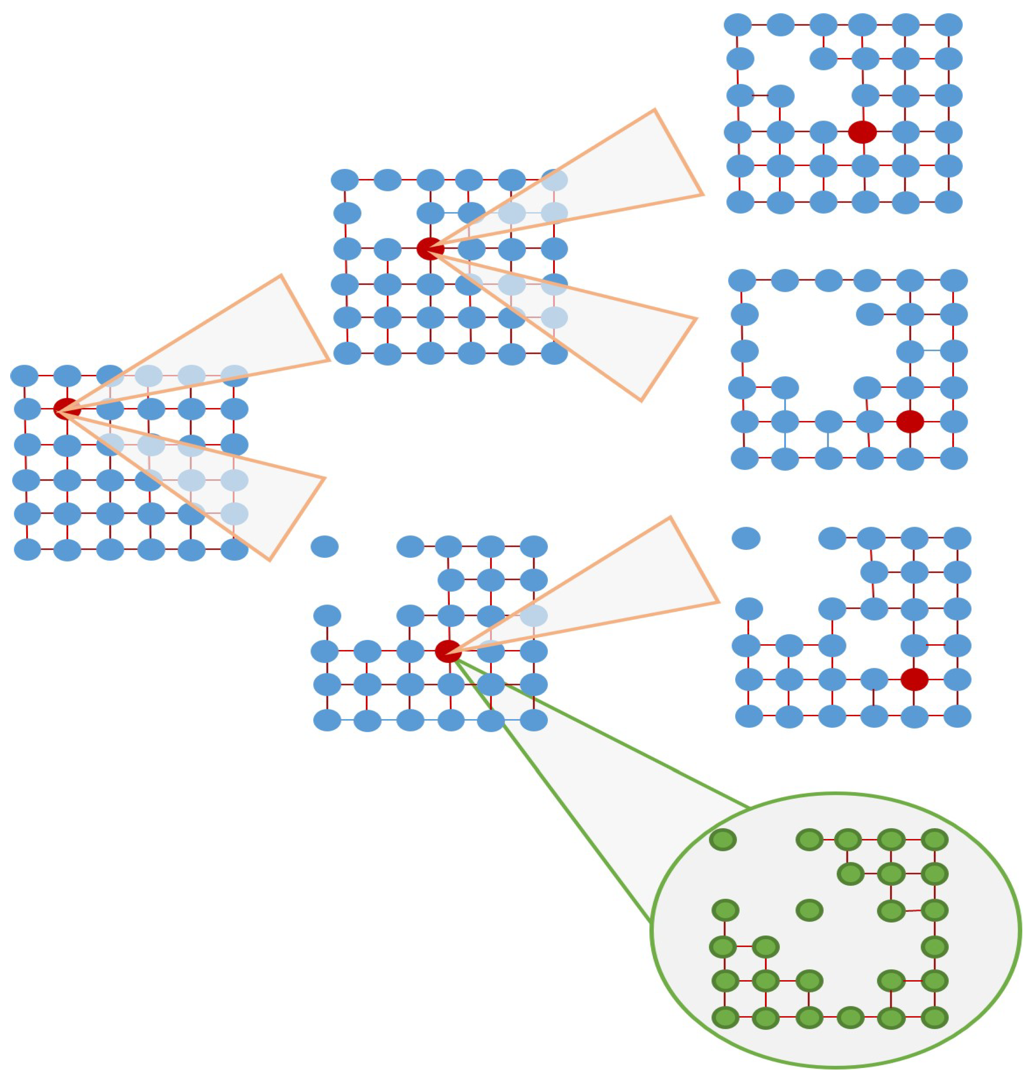
Applying the vertex division rule to v results in the creation of two new child nodes for the enumerative tree, $v_1$ and $v_2$, which branch out from the current node. The subgraph linked to $v_1$ is defined as $G_1=(G-v)$. Meanwhile, the subgraph linked to $v_2$ is defined as $G_2=(G-N\left[v\right])$.

At this point, a comparable problem to the original problem for each subgraph $G_i,i=1,2$ is built, akin to the issue faced with the original grid G. If the problem is solved recursively and its solution denoted as $r_i$, then the overall solution for $r=i\left(G\right)$ is given by $r=r_1+r_2$. The described process establishes an enumerative tree, where the leaves represent base subgraph instances.

This branching process continues until a subgraph associated with a child-node-based instance $G_p$ is obtained. A primary feature of any base instance $G_p$ is the absence of a vertex $u\in V\left(G_p\right)$ that is incident to four internal faces, except in the case where the subgraph is made up of exactly four adjacent tiles. In this scenario, the current subgraphs are recognized as a base case that will be associated with a child node of the enumerative tree. In Figure 4, the enumerative tree built by the BB algorithm when it is applied to the grid $G_{6,6}$ is illustrated.

In the previous section, it has been shown how the computation of $i\left(G_p\right)$ for the fundamental prime graph $G_p$ can be achieved in linear time with respect to its number of edges. This is possible because these fundamental prime graphs can be considered as outerplanar graphs, as mentioned in [22,23]. Let $k=(n-1)·(m-1)$ be the number of internal square faces of the input grid $G_{m,n}$, and let $H\left(B_G\right)=\{G_p:G_p$ represent the graph linked to a leaf node in the enumerative tree.}. After $B_G$ has been built, the following value is computed: $i\left(G\right)={\Sigma }_{G_p\in H\left(B_G\right)}i\left(G_p\right)$.

Since the computation for each $i\left(G_p\right)$ can be carried out in linear time, the overall time complexity of $i\left(G\right)$ is contingent upon the number of nodes in the enumerative tree. The time complexity of the branch-and-bound procedure results from the number of nodes formed by the recurrence $i\left(G\right)=i(G-\{u\left\}\right)+i(G-N[u\left]\right)$. The branching rule encompasses different scenarios depending on the number of internal faces incident to the vertices in $N\left[u\right]$. In the best-case scenario, $N\left[u\right]$ may be incident to eight tiling faces. In such cases, the decomposition rule, determined by the number of rectangles being decomposed, follows the recurrence: $T\left(k\right)=T(k-8)+T(k-3)$.

Nevertheless, in the worst-case scenario, if G does not align with an optimal case, then $N\left[u\right]$ must be incident to at least five internal faces. In such situations, the vertex division rule, as expressed by the number of rectangles being decomposed, is defined by the following recurrence:

$$T\left(k\right)=T(k-5)+T(k-3)$$

(4)

The aim is to find a solution in the form of $x^k=T\left(k\right)$. Upon substituting this expression into the preceding recurrence relation (4), the characteristic polynomial $P\left(x\right)=x^5-x^2-1$ is obtained. The five roots $r_i,i=1,\dots ,5$ of this polynomial correspond to solutions in the form of $T\left(k\right)=r_i^k$.

Given the focus is on the asymptotic behavior of the recurrence $T\left(k\right)$, the real root $r_1$ is exclusively considered with the condition $|r_1|\ge |r_i|,i=2,\dots ,5$. In this scenario, the maximum real root is approximately $r_1\approx 1.194$. Consequently, a worst-case upper bound of $O(r_1^k·poly\left(k\right))$ is derived, where the expression $poly\left(k\right)$ is a polynomial function accounting for the time processing of the basic case in the proposal. Therefore, the total time complexity for the branch-and-bound approach has an upper bound of $O(1.{1939}^k·poly\left(k\right))=O(1.{1939}^{(m-1)·(n-1)}·poly(m,n))$.

On the other hand, the classic transfer matrix approach involves constructing an initial matrix with dimensions of $F_{m+2}$ rows and $F_{m+2}$ columns, where $F_{m+2}$ denotes the $(m+2)$-th Fibonacci number. The rows and columns are labeled with $(m+1)$-vectors consisting of zeros and ones. Let S be an independent set of an input grid of m rows and n columns $\left(G_{m,n}\right)$, and let $C_m$ be the set of all $(m+1)$ vectors v of zeroes and ones, in which two consecutive ones are prohibited, and where a one indicates that its corresponding vertex is in S, and a zero indicates that the vertex is not in S. The cardinality of the set of these vectors is $F_{m+2}$, where $F_{m+2}$ corresponds with the $m+2$-th Fibonacci number.

Consider $T_m$ as a symmetric matrix with dimensions $F_{m+2}\times F_{m+2}$, comprising elements of zeroes and ones. The indexing of both rows and columns of $T_m$ are based on the vectors from $C_m$.

The requirement for vectors u and v within $C_m$ to constitute a potential consecutive pair of columns in an independent set of $G_{m,n}$ is precisely defined by the absence of shared positions containing the value 1. In other words, it is necessary that the dot product of u and v equals 0, employing the conventional dot product of vectors over the real numbers. Then, the entry of $T_m$ in position (u, v) is 1, if $u·v=0$; otherwise, it is 0. $T_m$ is called the transfer matrix of $G_{m,n}$. Then, $T_m$ has $F_{m+2}·F_{m+2}$ inputs with values of zeroes and ones.

The number of independent sets of the grid graph $G_{m,n}$ is the result of the sum of all entries of the n-th power matrix $T_m^n$, i.e., $i\left(G_{m,n}\right)={\mathbf{1}}^t{T}_m^n\mathbf{1}$, where 1 is the $F_{m+2}$ vector whose entries are all ones.

Analyzing the complexity time of the computation of ${\mathbf{1}}^t{T}_m^n\mathbf{1}$, the generation of the initial matrix $T_m$ exclusively entails an order of $O({\left(F_{m+2}\right)}^2·(m+1))$ dot products involving $m+1$-vectors across the real number domain. Afterward, the computation of $T_m^n$ request of an order of $O\left({\left(F_{m+2}\right)}^{3n}\right)$ multiplications among integers, and if the asymptotic behavior of the Fibonacci numbers is considered, the previous upper bound is rewritten as $O(\left({\left(1.618\right)}^{(m+2)·\left(3n\right)}\right)$ multiplications among integers, considering and approximation to the golden ratio of (1.618). The aforementioned upper bound complexity can be diminished to $O\left({\left(1.618\right)}^{(m+2)·\left(2.81n\right)}\right)$ integer multiplications through the utilization of the Strassen matrix-multiplication algorithm. In any case, the application of the transfer matrix method for computing $i\left(G_{m,n}\right)$ results in an exponential upper bound on both dimensions m and n of the grid.

When contrasting the upper bound of the time complexity derived from both approaches, the transfer matrix method and the branch-and-bound method, it is evident that the branch-and-bound method has significantly enhanced the time complexity in computing the M-S index on grid graphs. This improvement is attributed to the reduction in the base value as well as the exponentiated function’s superscript values being notably reduced compared to those associated with the transfer matrix method.

While the branch-and-bound method is applicable to any graph, its application specifically to square grid graphs results in an accelerated computational time for computing the M-S index of the input graph. This is achieved by judiciously selecting the vertex in the grid to implement the vertex division rule. Furthermore, the computational time analysis presented here focuses on input instances comprising only grid graphs as input to the branch and bound algorithm.

Indeed, the branch-and-bound method can operate seamlessly on irregular grids or variations of grids, such as the Aztec diamond graphs [7], which is a graph with vertices incident to more than three internal faces. However, while the proposal still exhibits an exponential time complexity, it lacks the explosive combinatorial nature associated with the classic transfer matrix method, a method that was specially designed to compute the number of independent sets in grid graphs.

6. Conclusions

A branch-and-bound algorithm to calculate $i\left(G_{m,n}\right)$ for grid graphs where m represents the number of rows and n represents the number of columns has been designed. The selected branching rule is widely recognized as the vertex reduction rule. The vertex v chosen for the reduction rule within the current subgraph of $G_{m,n}$ must meet the criterion of having $N\left[v\right]$ incident to a minimum of five internal faces. This strategy entails decomposing the initial grid until reaching the basic cases of the original problem. These basic cases may be either outerplanar subgraphs or subgrids where no neighborhood is incident to a minimum of five internal faces.

Three fundamental counting rules that enable the counting of independent sets in polynomial time for basic graph topologies have been established. These rules work as long as the basic graph is traversed by a Hamiltonian path. Indeed, these counting rules can be applied to compute the number of independent sets for more general topologies than grid graphs. The time complexity of the resulting algorithm for computing the Merrifield–Simmons index in grid graphs is significantly lower compared to the traditional transfer matrix method, which is specifically tailored for computing the number of independent sets in such graphs.

Furthermore, the proposed algorithm exhibits more widespread applicability than those algorithms designed exclusively for calculating the Merrifield–Simmons index in grid graphs, such as the transfer matrix method or more recent thread-based proposals. Indeed, the algorithmic approach developed in this work can be extended to various grid-like graph classes, including irregular grids, general polygonal face grids, and Aztec diamond graphs, or to processing benzenoid systems. This versatility is attributed to the general application of the ramification vertex rule across all classes of graphs.