Article

Gaussian Mixture Estimation from Lower-Dimensional Data with Application to PET Imaging

1
Faculty of Forestry and Wood Technology, University of Zagreb, 10000 Zagreb, Croatia
2
Faculty of Electrical Engineering and Computing, University of Zagreb, 10000 Zagreb, Croatia
*
Author to whom correspondence should be addressed.
Mathematics 2024, 12(5), 764; https://doi.org/10.3390/math12050764
Submission received: 16 January 2024 / Revised: 22 February 2024 / Accepted: 1 March 2024 / Published: 4 March 2024
(This article belongs to the Special Issue Inverse Problems and Imaging: Theory and Applications)

Abstract

:
In positron emission tomography (PET), the original points of emission are unknown, and the scanners record pairs of photons emitting from those origins and creating lines of response (LORs) in random directions. This presents a latent variable problem, since at least one dimension of relevant information is lost. This can be solved by a statistical approach to image reconstruction—modeling the image as a Gaussian mixture model (GMM). This allows us to obtain a high-quality continuous model that is not computationally demanding and does not require postprocessing. In this paper, we propose a novel method of GMM estimation in the PET setting, directly from lines of response. This approach utilizes some well-known and convenient properties of the Gaussian distribution and the fact that the random slopes of the lines are independent from the points of origin. The expectation–maximization (EM) algorithm that is most commonly used to estimate GMMs in the traditional setting here is adapted to lower-dimensional data. The proposed estimation method is unbiased, and simulations and experiments show that accurate reconstruction on synthetic data is possible from relatively small samples.

1. Introduction

Positron emission tomography (PET) is an imaging technique that uses radioisotopes (i.e., radiotracers) and rings of crystal detectors. The injected tracer, designed to attach itself to the object or process of interest, decomposes and emits pairs of photons in opposite directions, creating a line that the scanner detects and records as an event when two crystals are activated simultaneously [1]. In a fully three-dimensional scanner, all possible pairs of crystals create tubes, i.e., volumes of response (VORs), which capture the events. Alternatively, in the two-dimensional case, pairs of crystals form lines of response (LORs), and the scanner detects events along a single plane, which are later used to reconstruct the 3D image.
Traditional reconstruction methods in tomography generally fall under two categories—analytic or iterative algorithms [2,3]. Analytic methods are based on the Fourier transform and its inverse, using the projection-slice theorem (sometimes called the central section theorem) [4]. The most used is the filtered back projection, also known as the Radon inverse transform [5,6]. This method filters the projections to reduce noise and artifacts and then backprojects them along different angles, and is still widely used in CT scan reconstructions [7]; however, the resulting image is of lower resolution compared with other methods. Similar traditional methods, now outperformed by others, are back projection filtering, where the filtering step occurs after the back projection, and the Fourier transform method that transforms the data into the frequency domain, which manipulates it there and then transforms it back to the spatial domain [8]. These methods are computationally simple and fast; however, they assume that the data are noise-free and they do not account for randomness or stochastic variability. This means that they require a lot of pre- and postprocessing in order to obtain good image quality. By definition, the inverse problem is ill-posed and is therefore very sensitive to small perturbations in the original data. Before reconstruction, raw data are corrected for attenuation and noise, and filters can be applied in both the spatial and frequency domains. Filtering is also commonly applied at the postprocessing stage, as well as various regularization techniques that enforce smoothness and penalize undesired properties [9].
The main problem in PET image reconstruction is attenuation, i.e., the loss of detection of true coincidence events due to photons being absorbed in the body, scattering out of the field of view or changing course after collision. There are many attenuation correction techniques using either additional CT scans or properties of the PET scanner itself. In clinical settings, the choice of method depends on resources like computational power and availability of combined PET/CT scanners [10,11]. In recorded data, one of the consequences of attenuation is wrongly recorded or false events. When one or both of the photons in a pair change course, it activates the wrong crystal, and the resulting measurement is a line that does not contain the real point of origin. This new event differs from the real unrecorded one, and depending on the size of the error, i.e., the angle by which the course had changed, it is considered as photon noncollinearity (small) or scattered coincidence (large difference). Finally, given that the scanner records events at discrete times, it is possible for two or more events to occur “at the same time”. If more than one pair of crystals is activated at the same time, the scanner can pair them incorrectly, resulting in random coincidences [12].
With increased computational powers, iterative models became widespread at the end of the 20th century [13,14,15,16,17,18] and are still most widely used, often in combination with analytical techniques [3]. They are usually based on the expectation–maximization (EM) algorithm [19], traditionally using maximum likelihood estimation (MLEM) [20]. In general, these techniques discretize the image domain into distinct pixels or voxels and iteratively improve their estimation of pixel/voxel values. In the maximum likelihood approach, the Poisson distribution is most commonly used to model the number of times each detector pair would record an event. The MLEM was later updated to accelerate convergence with methods that use only parts of the data at each step, e.g., the ordered subsets EM algorithm (OSEM) [21]. These methods are more resistant to noise, but they still require postfiltering for denoising, as well as some regularization methods to counteract issues arising from ill-conditioned problems [22].
It should be mentioned that recent progress in medical imaging has been achieved by utilizing deep learning and AI-based solutions [23,24,25,26]. This new approach is proving to be most useful in solving previously unfeasible problems that are ill-posed or lacking the mathematical framework, but in standard image reconstruction problems, traditional methods are still competitive [27]. Deep learning methods can be used to improve existing methodology, e.g., by denoising the data [28], but a full implementation of AI-based models is limited by evaluation and interpretability issues [29,30] and computational memory [31].
Standard modern algorithms in image reconstruction include some sort of stochastic model that utilizes prior or additional knowledge. The Gaussian mixture model (GMM) has been proven suitable for a variety of segmentation problems [32,33,34]. In PET reconstruction problems, the original data (i.e., points of origin) are unobserved, so GMMs are used to model activity at points of observation, with spatial dependence modeled by Markov random fields [35,36,37]. An alternative approach is to model the unknown points of origin using GMMs directly by utilizing nice statistical properties of the Gaussian distribution to overcome missing information [38,39]. This novel strategy yields a continuous model of infinite resolution that can be reconstructed directly and evaluated at any point in the imaging plane. Furthermore, it requires a much smaller sample than traditional methods, which means that scanning requires lower doses of radiation and less time in the scanner.
This paper presents a new method for estimating Gaussian parameters from lower-dimensional data. Using synthetic measurements, we demonstrate how this approach can be used to estimate a full Gaussian mixture model on PET data using an iterative EM-like algorithm. In Section 2, we show how to estimate parameters of a single distribution, and in Section 3, we expand this idea to simultaneously estimate parameters of a mixture of Gaussian distributions. Section 4 demonstrates the approach on synthetic data, and a discussion concludes the paper.

2. Gaussian Estimation from PET Data

Original PET data are a set of events recorded when the scanner registers a pair of photons activate two crystals simultaneously. These events can be represented as lines connecting the pairs of crystals, while the points of origin remain unknown (Figure 1).
Traditionally, these data would be stored as a histogram of events across all angles, called a sinogram. The original location of the tracer that emitted the photons would then be reconstructed using analytic or iterative methods, and corrected for measurement errors. In this paper, we assume that the points of origin follow a known distribution and estimate the parameters of that distribution directly from the lines.
To start, assume that the location of any point x , where a positron is annihilated and emits the pair of photons, follows a single Gaussian distribution with the parameters μ and Σ . Note that the following calculations are performed in the 2D setting for simplicity, but analogous claims are true in the three-dimensional case. An event, i.e., line, in the 2D setting can be represented by two parameters, and possible representations are of course interchangeable. In this work, we will observe the line slope k = tan φ , where φ π 2 , π 2 , and an intercept l. Therefore, N events give us a series of N equations:
y = tan φ i · x + l i , i = 1 , ߪ , N .

2.1. Estimation of μ

It has been shown that the mean μ can be estimated in many ways, e.g., from intersections of lines [40] or directly from the sinogram [39]. For this part, we follow the methodology from [38], which shows that the mean is accurately estimated as the point that minimizes the total squared Euclidean distance from all events. If we denote a i = [ tan φ i 1 ] T , the location of this point can be calculated as follows:
μ T = i = 1 N l i m i · i = 1 N 2 M i N i 1 ,
where
M i m i = B i 2 I a i a i T 0 2 I 0 1 0 0 1 0 0 , N i 0 = B i T 2 I 0 I ˜ 1 0 0 1 0 0 , B i = 2 I a i a i T 0 1 T · I ˜ and I ˜ = I 0 0 0 .
Once the center has been estimated, we can also find the points on each line that are nearest to it. Consider the i-th event and the original unknown point of origin x i = [ x i , y i ] T . Equation (1) can also be written as follows:
cos φ i ( y y i ) = sin φ i ( x x i ) .
Any line perpendicular to the i-th line has the slope 1 tan φ i = cos φ i sin φ i , and especially one that goes through μ satisfies the following:
sin φ i ( y μ y ) = cos φ i ( x μ x ) .
For simplicity, denote s i = sin φ i and c i = cos φ i . If we omit the index i in the coordinates for legibility, denote the point on line i nearest to the center μ as y i = [ x s , y s ] T . This point satisfies (3) and (4), which can be written in matrix form:
s i c i c i s i · x s y s = s i c i 0 0 0 0 c i s i · x i y i μ x μ y ,
and gives the following solution:
y i = x s y s = s i 2 x i s i c i y i + c i 2 μ x + s i c i μ y s i c i x i + c i 2 y i + s i c i μ x + s i 2 μ y .
It is straightforward to show from (5) that E ( y i ) = μ as well.

2.2. Estimation of Σ

Statistical properties of the set of “nearest points” found in the previous section by (5) can be connected to the statistical properties of the original set of (unknown) points, which will enable us to estimate the original covariance matrix:
Σ = Σ 11 Σ 12 Σ 12 Σ 22 .
Consider the ith point of origin x i = [ x i , y i ] T from a Gaussian distribution with the parameters ( μ Σ ) and its corresponding point nearest to the center, y = [ x s , y s ] T . We will now show how their covariance matrix C = E ( ( y μ ) · ( y μ ) T ) relates to the original covariance matrix Σ . First, assume for simplicity that μ = [ 0 , 0 ] T , i.e., that the measurements have been centered. Equation (5) can now be written as follows:
x s y s = s i 2 x i s i c i y i s i c i x i + c i 2 y i = s i 2 s i c i s i c i c i 2 · x i y i .
Then we have the following:
C = E ( [ x s , y s ] T · [ x s , y s ] ) = E s 11 s 12 s 21 s 22 ,
where
s 11 = s i 4 x i 2 2 s i 3 c i x i y i + s i 2 c i 2 y i 2 s 12 = s i 3 c i x i 2 + 2 s i 2 c i 2 x i y i c i 3 s i y i 2 = s 21 s 22 = s i 2 c i 2 x i 2 2 s i c i 3 x i y i + c i 4 y i 2 .
This can be expressed in matrix form as follows:
s 11 s 12 s 22 = s i 4 2 s i 3 c i s i 2 c i 2 s i 3 c i 2 s i 2 c i 2 c i 3 s i s i 2 c i 2 2 s i c i 3 c i 4 · x i 2 x i y i y i 2 .
The key observation here is that the first matrix on the right-hand side is a function only of the angles at which the lines appear. These angles are random, uniformly distributed, and independent from the points of origin. Therefore, when taking the expectation of (6), it can be separated into a product of two expectations:
E s 11 s 12 s 22 = E s i 4 2 s i 3 c i s i 2 c i 2 s i 3 c i 2 s i 2 c i 2 c i 3 s i s i 2 c i 2 2 s i c i 3 c i 4 · E x i 2 x i y i y i 2 .
Since the angle φ is uniformly distributed over π 2 , π 2 , we can calculate, e.g., as follows:
E ( s i 4 ) = π 2 π 2 sin 4 φ d φ = 3 8 , E ( 2 s i 3 c i ) = 2 π 2 π 2 sin 3 φ cos φ d φ = 0 ,
and similar calculations for other expressions in (7) yield the following:
E s i 4 2 s i 3 c i s i 2 c i 2 s i 3 c i 2 s i 2 c i 2 c i 3 s i s i 2 c i 2 2 s i c i 3 c i 4 = 3 8 0 1 8 0 1 4 0 1 8 0 3 8 = : M .
To estimate the original covariance matrix, we begin by estimating the covariance matrix of the (centered) nearest points:
C ^ = i = 1 N y i y i T = c 11 c 12 c 21 c 22 .
From (7) and (8), the following is derived:
σ x 2 σ x y σ y 2 = E x i 2 x i y i y i 2 = M 1 · E s 11 s 12 s 22 = 3 0 1 0 4 0 1 0 3 · E s 11 s 12 s 22 ,
which means the following:
σ ^ x 2 σ ^ x y σ ^ y 2 = 3 0 1 0 4 0 1 0 3 · c 11 c 12 c 22 .

3. Gaussian Mixtures in PET Imaging

3.1. Gaussian Mixture Model

The Gaussian mixture model [41] assumes that a d-dimensional observation x is generated from a mixture of K Gaussian densities, as follows:
p ( x | π k , μ k , Σ k ) = k = 1 K π k f G ( x | μ k , Σ k ) ,
where π i ( i = 1 , . . . , K ) are the weights of each Gaussian component, and f G ( x | μ k , Σ k ) are the component densities. Each density is a d-variate Gaussian function of the following form:
f G ( x | μ k , Σ k ) = 1 ( 2 π ) d | Σ k | exp 1 2 ( x μ k ) T Σ k 1 ( x μ k ) ,
and we assume that x originates from exactly one of the components (clusters). This is a model with a latent (hidden) variable that records component membership. If we denote this variable by Z, we can write π k = P ( Z = k ) as the probability that x belongs to the k-th Gaussian component, with k = 1 K π k = 1 . The model parameters that need to be estimated are the mean vectors { μ k } , covariance matrices { Σ k } , and mixture weights { π k } for each Gaussian component.
Even in the traditional setting, this is a model with latent variables. Since the component membership of each observation is unknown, the maximum likelihood approach will not provide a closed-form solution. Several estimation methods have been proposed, and the most common one is the iterative expectation–maximization (EM) algorithm [19]. In the following section, we will adapt this approach to our estimation method from Section 2.

3.2. EM-like Algorithm

Broadly, the original EM algorithm iterates between two steps:
E:
Given a set of parameters Θ = { π k , μ k , Σ k } , calculate the probability that each observation x ( i ) originated from the k-th component:
h k ( i ) = P ( Z i = k | x ( i ) ) = p x ( i ) | μ k , Σ k π k j = 1 K p x ( i ) | μ j , Σ j π j .
These probabilities are sometimes also called responsibilities, or posterior probabilities.
M:
Given the set of probabilities { h k ( i ) } , estimate the parameters of each component. This step is named after the maximum likelihood method that is used to estimate the parameters.
The algorithm can be initialized either from a random set of parameters θ or by randomly assigning the probabilities h. Note that, in our approach, the estimation is not derived directly from max likelihood given that we do not have the original data; nevertheless, we can adapt this algorithm to achieve satisfactory results.

3.2.1. Initialization

To ensure a “smart” initialization that will minimize the number of iterations later, we adapt the approach from [39]. This part combines k-means(-like) clustering with parameter estimation from the previous section (Matlab (R2022b) code for all experiments can be made available on request from the corresponding author).
  • Each line is initially randomly assigned to exactly one component, while ensuring that each component has approximately the same number of lines.
  • Mean vectors of each component are estimated as described in Section 2.
  • Lines are reassigned to the component whose estimated mean vectors are nearest to them in terms of Euclidean distance. In this step, we still adhere to the so-called hard classification; i.e., each line is assigned to only one component.
    Steps 2 and 3 are repeated until the changes in mean vectors are sufficiently small.
Once the hard classification and reassignment are completed, the initial covariances are estimated once from all lines assigned to them following the methodology from Section 2. Initial weights { π k } are calculated as the relative size of the components, i.e., the proportion of all lines that are assigned to a specific component.

3.2.2. E Step

As in the traditional algorithm, given a set of parameters θ = { π k , μ k , Σ k } , this step calculates the probabilities { h k ( i ) } that the i-th observation belongs to the k-th component. If we denote by γ i our i-th observation (i.e., some parametrization of the line), we need to calculate the following:
h k ( i ) = P ( Z i = k | γ i ) = p γ i | μ k , Σ k π k j = 1 K p γ i | μ j , Σ j π j .
The term p γ i | μ k , Σ k is the integral of the density along the following line:
p γ i | μ k , Σ k = γ i f G ( x | μ k , Σ k ) d γ i ,
where f G again denotes the (bivariate) Gaussian density. For a quicker computation, we can utilize the following nice properties of the Gaussian distribution:
  • A Gaussian distribution retains properties when rotated.
  • Marginal distributions of a Gaussian are again Gaussian.
If an event is at an angle φ , rotating the coordinate system by ψ = π 2 φ makes it parallel to the y-axis and defined by its abscissa coordinate x = l sin ψ . The coordinates of the center μ and covariance Σ are now R μ and R Σ R T , where R denotes the rotation matrix. Given that the line is now parallel to the y-axis, the integral along the line simply gives us the marginal distribution in the first coordinate (in our new coordinate system):
p γ i | μ k , Σ k = f G ( l sin ψ | ( R i μ k ) 1 , ( R i Σ k R i T ) 11 ) ,
where R i denotes the operator of rotation by ψ i and f G is now the univariate Gaussian density. In the two-dimensional setting, this can be calculated as follows:
p γ i | μ k , Σ k = f G ( l sin ψ | cos ψ i μ x sin ψ i μ y , cos 2 ψ i Σ 11 2 cos ψ i sin ψ i Σ 12 + sin 2 ψ i Σ 22 ) .
For more details, see [38], and Figure 2 illustrates the idea.

3.2.3. M-like Step

Given the estimated posterior probabilities { h k ( i ) } and previous component centers { μ k } , we re-estimate the parameters. For each component, we have the following:
  • Find the nearest points y i to the (previous iterations’) center for each line.
  • Calculate the weighted mean and covariance of y i s with probabilities h as weights:
    μ k = i h k ( i ) y i i h k ( i ) , C k = i h k ( i ) ( y i μ k ) ( y i μ k ) T i h k ( i ) .
  • Calculate Σ k from C k as in Section 2.
  • Mixture weights π k are calculated, as in the original EM algorithm, as the proportion of all lines (events) assigned to each component: π k = 1 N i = 1 N h k ( i ) .
The E and M steps are repeated until there are only small changes between iterations, specifically until there is virtually no change in estimated weight of each component. The following section evaluates our approach, both for a single component and in the mixture setting.

4. Experiments and Results

4.1. Single-Component Estimation

To demonstrate that the approach described in Section 2 correctly estimates the covariance matrix, we experimented with five covariances representing different shapes and types:
Σ 1 = 0.0625 0 0 0.0625 , Σ 2 = 0.04 0.03 0.03 0.09 , Σ 3 = 0.04 0.006 0.006 0.01 Σ 4 = 0.09 0.0135 0.0135 0.09 , Σ 5 = 0.04 0.004 0.004 0.04
Note that the corresponding correlation coefficients are as follows:
ρ 1 = 0 , ρ 2 = 0.5 , ρ 3 = 0.3 , ρ 4 = 0.15 , ρ 5 = 0.1 .
Estimation was performed n = 100 times for each covariance type and for sample sizes N varying from N = 1000 to N = 100 , 000 . For each iteration, the relative error was calculated as follows:
Rel . error = | | Σ S | | F | | Σ | | F ,
where | | · | | F denotes the Frobenius norm of the matrix. Figure 3 shows the average relative error for all covariance types and all values of N. We see that accurate reconstruction is achieved even from small (in the context of PET imaging) samples, starting with approximately N = 2000 , regardless of the covariance type.

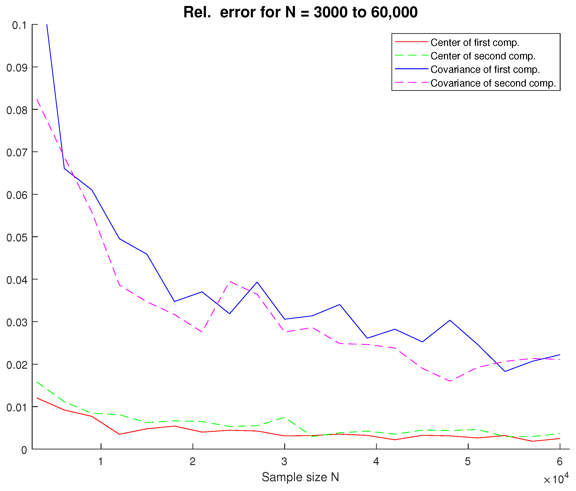
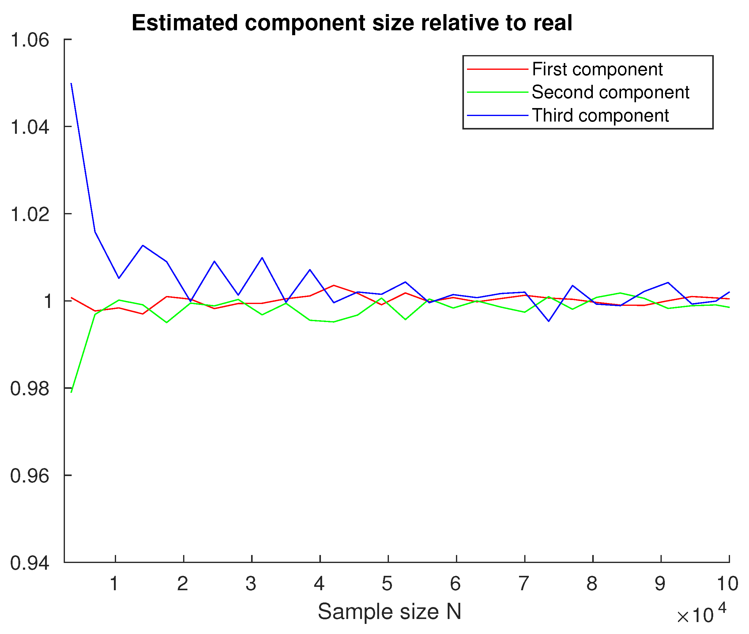
4.2. Gaussian Mixture Estimation

To illustrate the effectiveness of the proposed algorithm, several experiments were conducted for two and three components. First, for K = 2 , the following parameters were set:
N = N 1 + N 2 , N 2 N 1 = 5 7 , μ 1 = 0 1 , μ 2 = 1 0 , Σ 1 = 0.0625 0 0 0.0625 , Σ 2 = 0.04 0.03 0.03 0.09 .
The total sample size N varied from 3000 ( N 1 = 1750 , N 2 = 1250 ) to 60,000 ( N 1 = 35,000, N 2 = 25,000). Each experiment was repeated 100 times, and the results are given in Figure 4.
The estimated component weight was calculated as follows:
N ^ k = i = 1 N h k ( i ) ,
where h k ( i ) was calculated as in (11). The criterion for stoppage was that each component weight changed by less than 10 between iterations. Note that the algorithm performed only a few (approx. 4–5) iterations each time before there was virtually no change in component weights. Figure 5 shows the ratio of relative and actual component sizes N k ^ / N k , calculated as an average over all simulations for each sample size. Clearly, component weights are well estimated regardless of the total sample size.
Similar experiments were performed for K = 3 components with varying sizes and shapes. The following parameters were used:
N = N 1 + N 2 + N 3 , N 2 N 1 = 5 7 , N 3 N 1 = 2 7 , μ 1 = 0 1 , μ 2 = 1 0 , μ 3 = 1.25 1 Σ 1 = 0.0625 0 0 0.0625 , Σ 2 = 0.04 0.03 0.03 0.09 , Σ 3 = 0.04 0.006 0.006 0.01 .
The total sample size N varied from 3500 ( N 1 = 1750 , N 2 = 1250 , N 3 = 500 ) to 105,000 ( N 1 = 52,500, N 2 = 37,500, N 3 = 15,000). Each experiment was repeated 100 times, and Figure 6 depicts the mean relative errors calculated as in (13) using the Euclidean norm for centers. The centers are well estimated even for very small samples, as well as the covariance of the smallest (third) component. A slightly larger sample is required for accurate covariance estimation for components with larger proportions of weight. Still, a total sample size of ≈100,000 is still significantly smaller than the traditional PET measurement size.
As in the two-component case, Figure 7 shows that component sizes (weights) were correctly estimated even from small sample sizes. It can also be noted that the number of iterations increased approximately from 10 to 20 with growing sample sizes, with no simulation exceeding 22 iterations per component. The results presented here are representative of many simulations for different types and combinations of covariance matrices, which were omitted here for brevity. Some additional similar results can be found in Appendix A for comparison.
Finally, Figure 8 illustrates the similarity between the original Gaussian model, i.e., the unknown components, and the proposed estimated reconstruction.

4.3. Noise Resistance

To demonstrate how this approach would behave in a more realistic setting, two types of noise have been simulated. First, a noise effect was added to some points of origin. Points were generated from three mixture components as described in Section 4.2, and a certain number of them were offset by error:
x ˜ = x + ε , ε N 0 , σ I .
Recall that when a photon slightly changes course, the resulting measurement is an event that is “close” to the original point, but does not pass through it. Since line directions are random and independent from the points themselves, this type of noise mimics the occurrence of photon noncollinearity—an event is recorded that does not contain the real point of origin, but is close to it. The parameters σ = 0.005 and σ = 0.01 were selected to represent approximately 10% and 20% variability of the original data, respectively, and a randomly selected subset of 10% of data was “noisified”. The results are shown in Figure 9. Compared with Figure 6, we see that the error decays more slowly, but satisfactory precision is still achieved.
To assess how the estimation behaves with different quantities of photon noncollinearity, an error with σ = 0.005 was added to an increasing percentage of data (from 1% to 20%). This experiment was performed on a sample size N = 105,000, corresponding to component sizes of N 1 = 52,500, N 2 = 37,500, N 3 = 15,000, and the results are shown in Figure 10. The precision deteriorates with added noise, but even with 20% of noisy data, the error terms are still below 5%.
To represent random coincidences, additional false measurements were added to the original measurements. The points of origin were generated randomly within the scanner field of view and added to the real measurements. The algorithm was slightly modified to accommodate potential outliers. One of the oldest and simplest ideas is the so-called “three-sigma rule”, where measurements are classified as outliers if they are more than three standard deviations away from the mean [42]. Here, estimation was first performed on the full dataset. Then, each line was projected to one dimension as described in Section 3.2.2, along with the component means and variances (see Figure 2). If the line was more than three standard deviations away from all three components, it was classified as an outlier. Finally, the parameters were estimated again with the outliers omitted. The experiment was performed with the parameters as in Section 4.2 and the total sample size ranging from N = 3500 to N = 105,000, with 2% random events added. The results are shown in Figure 11. More advanced and precise outlier detection methods will be incorporated when the algorithm is applied to real data, but this demonstrates that the method on its own is robust for small amounts of random coincidences.
This section shows that the algorithm is resistant to a relatively small amount of noise and false measurements. Therefore, less pre- and postprocessing would be required to achieve accurate reconstruction, which is important given that excessive regularization risks losing important features of the data.

5. Conclusions

In this paper, we have presented a new way of estimating Gaussian parameters from lower-dimensional observations in the PET context. The EM algorithm is adapted for GMM estimation from projections, with experiments showing that accurate reconstruction is possible from relatively small samples. The method relies on the geometric properties of the Gaussian distribution, and simulations demonstrate that the obtained unbiased estimators quickly converge to real parameter values. Compared with traditional methods that estimate individual pixels (or voxels) and give quantized values, this approach results in a continuous model of the PET image.
The limitation of this work is that it was performed on synthetic measurements, and application to real data is the next step in ongoing research. This includes incorporating scanner properties [43], as well as some issues that traditionally arise when dealing with mixture models, such as determining the proper number of components [44]. As it stands, this manuscript serves as proof of concept and of the feasibility of the approach.
To the best of our knowledge, Gaussian mixture models have not yet been used in modeling PET images in this way, and estimating model parameters from data of this type is a new and unresearched topic. Given the significance and usefulness of Gaussian models in image reconstruction problems, these results are encouraging and imply efficient reconstruction from fewer measurements that are currently used. This would, of course, mean that accurate imaging could be achieved while exposing patients to significantly lower doses of radiation. Additionally, the method could be applied to an array of other mixture models where the distributions have similar properties to the Gaussian, thus expanding the types of images that can be reconstructed in this manner.

Author Contributions

Conceptualization, A.T. and D.S.; methodology, A.T. and D.S.; software, A.T. and D.S.; validation, A.T. and D.S.; formal analysis, A.T. and D.S.; investigation, A.T. and D.S.; writing—original draft preparation, A.T.; writing—review and editing, D.S.; visualization, A.T. and D.S.; supervision, A.T. and D.S.; project administration, A.T.; funding acquisition, D.S. All authors have read and agreed to the published version of the manuscript.

Funding

This work was supported by the Croatian Science Foundation under project IP-2019-04-6703.

Institutional Review Board Statement

Not applicable.

Data Availability Statement

The data presented in this study are available on request from the corresponding author.

Acknowledgments

The authors would also like to thank Tomislav Matulić for his help with algorithm implementation.

Conflicts of Interest

The authors declare no conflicts of interest.

Abbreviations

The following abbreviations are used in this manuscript:
PETpositron emission tomography
LORline of response
GMMGaussian mixture model
EMexpectation maximization
VORvolume of response

Appendix A

As mentioned earlier, the results in Section 4.2 represent similar results obtained for various combinations of covariance matrices, some of which are presented here for comparison.

Appendix A.1. Different Covariances

All parameters from Section 4.2 are repeated with different covariance matrices. Figure A1 shows average component sizes and estimation errors from 100 simulations, and the results are similar to Figure 6.
N = N 1 + N 2 + N 3 , N 2 N 1 = 5 7 , N 3 N 1 = 2 7 , μ 1 = 0 1 , μ 2 = 1 0 , μ 3 = 1.25 1 Σ 1 = 0.04 0 0 0.0625 , Σ 2 = 0.09 0.045 0.045 0.09 , Σ 3 = 0.04 0.03 0.03 0.01 .
Figure A1. (a) Estimatedto real component size ratio; (b) relative errors for three components.
Mathematics 12 00764 g0a1

Appendix A.2. Equal Component Sizes

All parameters from Section 4.2 remain the same, but components are generated to be of equal size. Component sizes vary from N i = 2000 to 40,000 ( N = 6000 to 120,000). Figure A2 shows average component sizes and estimation errors from 100 simulations.
N = N 1 + N 2 + N 3 , N 1 = N 2 = N 3 , μ 1 = 0 1 , μ 2 = 1 0 , μ 3 = 1.25 1 , Σ 1 = 0.0625 0 0 0.0625 , Σ 2 = 0.04 0.03 0.03 0.09 , Σ 3 = 0.04 0.006 0.006 0.01 .
Figure A2. (a) Estimated to real component size ratio; (b) relative errors for three components of the same size.
Mathematics 12 00764 g0a2

Appendix A.3. Four Components

Figure A3. (a) Estimated to real component size ratio; (b) relative errors for four components.
Mathematics 12 00764 g0a3
Finally, simulations were expanded to include four components. A representative result is presented below, with the parameters as follows:
N = N 1 + N 2 + N 3 + N 4 , N 2 N 1 = 5 7 , N 3 N 1 = 2 7 , N 4 N 1 = 3 7 , μ 1 = 0 1 , μ 2 = 1 0 , μ 3 = 1.25 1 , μ 4 = 0.6 1 Σ 1 = 0.0625 0 0 0.0625 , Σ 2 = 0.04 0.03 0.03 0.09 , Σ 3 = 0.04 0.006 0.006 0.01 , Σ 4 = 0.09 0.0135 0.0135 0.09 .
The total sample size varied from 4500 to 135,000, and the results are presented in Figure A3. They are (expectedly) slightly worse than the results for three components, but for larger sample sizes, sufficient accuracy is still achieved.

References

  1. Bailey, D.L.; Maisey, M.N.; Townsend, D.W.; Valk, P.E. Positron Emission Tomography; Springer: London, UK, 2005; Volume 2. [Google Scholar]
  2. Tong, S.; Alessio, A.M.; Kinahan, P.E. Image reconstruction for PET/CT scanners: Past achievements and future challenges. Imaging Med. 2010, 2, 529–545. [Google Scholar] [CrossRef]
  3. Reader, A.J.; Zaidi, H. Advances in PET image reconstruction. PET Clin. 2007, 2, 173–190. [Google Scholar] [CrossRef]
  4. Kinahan, P.E.; Defrise, M.; Clackdoyle, R. Analytic image reconstruction methods. In Emission Tomography; Elsevier: Amsterdam, The Netherlands, 2004; pp. 421–442. [Google Scholar]
  5. Natterer, F. The Mathematics of Computerized Tomography; Siam: Philadelphia, PA, USA, 1986; Volume 32. [Google Scholar] [CrossRef]
  6. O’Sullivan, F.; Pawitan, Y. Multidimensional Density Estimation by Tomography. J. R. Stat. Soc. Ser. B Methodol. 1993, 55, 509–521. [Google Scholar] [CrossRef]
  7. Singh, S.; Kalra, M.K.; Hsieh, J.; Licato, P.E.; Do, S.; Pien, H.H.; Blake, M.A. Abdominal CT: Comparison of adaptive statistical iterative and filtered back projection reconstruction techniques. Radiology 2010, 257, 373–383. [Google Scholar] [CrossRef] [PubMed]
  8. Alessio, A.; Kinahan, P. PET image reconstruction. Nucl. Med. 2006, 1, 4095–4103. [Google Scholar] [CrossRef]
  9. Ahn, S.; Leahy, R.M. Analysis of resolution and noise properties of nonquadratically regularized image reconstruction methods for PET. IEEE Trans. Med. Imaging 2008, 27, 413–424. [Google Scholar] [PubMed]
  10. Zaidi, H.; Montandon, M.L.; Alavi, A. Advances in attenuation correction techniques in PET. PET Clin. 2007, 2, 191–217. [Google Scholar] [CrossRef] [PubMed]
  11. Chow, P.L.; Rannou, F.R.; Chatziioannou, A.F. Attenuation correction for small animal PET tomographs. Phys. Med. Biol. 2005, 50, 1837. [Google Scholar] [CrossRef] [PubMed]
  12. Mincke, J.; Courtyn, J.; Vanhove, C.; Vandenberghe, S.; Steppe, K. Guide to plant-pet imaging using 11CO2. Front. Plant Sci. 2021, 12, 602550. [Google Scholar] [CrossRef] [PubMed]
  13. Levitan, E.; Herman, G.T. A Maximum a Posteriori Probability Expectation Maximization Algorithm for Image Reconstruction in Emission Tomography. IEEE Trans. Med. Imaging 1987, 6, 185–192. [Google Scholar] [CrossRef]
  14. Lewitt, R.M.; Matej, S. Overview of methods for image reconstruction from projections in emission computed tomography. Proc. IEEE 2003, 91, 1588–1611. [Google Scholar] [CrossRef]
  15. Leahy, R.M.; Qi, J. Statistical approaches in quantitative positron emission tomography. Stat. Comput. 2000, 10, 147–165. [Google Scholar] [CrossRef]
  16. Meikle, S.R.; Hutton, B.F.; Bailey, D.L.; Hooper, P.K.; Fulham, M.J. Accelerated EM reconstruction in total-body PET: Potential for improving tumour detectability. Phys. Med. Biol. 1994, 39, 1689. [Google Scholar] [CrossRef] [PubMed]
  17. Zaidi, H.; Abdoli, M.; Fuentes, C.L.; El Naqa, I.M. Comparative methods for PET image segmentation in pharyngolaryngeal squamous cell carcinoma. Eur. J. Nucl. Med. Mol. Imaging 2012, 39, 881–891. [Google Scholar] [CrossRef] [PubMed]
  18. Hatt, M.; Le Rest, C.C.; Turzo, A.; Roux, C.; Visvikis, D. A fuzzy locally adaptive Bayesian segmentation approach for volume determination in PET. IEEE Trans. Med. Imaging 2009, 28, 881–893. [Google Scholar] [CrossRef] [PubMed]
  19. Dempster, A.P.; Laird, N.M.; Rubin, D.B. Maximum likelihood from incomplete data via the EM algorithm. J. R. Stat. Soc. B 1977, 39, 1–38. [Google Scholar] [CrossRef]
  20. Shepp, L.A.; Vardi, Y. Maximum likelihood reconstruction for emission tomography. IEEE Trans. Med. Imaging 1982, 1, 113–122. [Google Scholar] [CrossRef] [PubMed]
  21. Hudson, H.M.; Larkin, R.S. Accelerated image reconstruction using ordered subsets of projection data. IEEE Trans. Med. Imaging 1994, 13, 601–609. [Google Scholar] [CrossRef]
  22. Qi, J.; Leahy, R.M. Iterative reconstruction techniques in emission computed tomography. Phys. Med. Biol. 2006, 51, R541. [Google Scholar] [CrossRef]
  23. Kim, K.; Wu, D.; Gong, K.; Dutta, J.; Kim, J.H.; Son, Y.D.; Kim, H.K.; El Fakhri, G.; Li, Q. Penalized PET Reconstruction Using Deep Learning Prior and Local Linear Fitting. IEEE Trans. Med. Imaging 2018, 37, 1478–1487. [Google Scholar] [CrossRef]
  24. Wang, Y.; Yu, B.; Wang, L.; Zu, C.; Lalush, D.S.; Lin, W.; Wu, X.; Zhou, J.; Shen, D.; Zhou, L. 3D conditional generative adversarial networks for high-quality PET image estimation at low dose. Neuroimage 2018, 174, 550–562. [Google Scholar] [CrossRef]
  25. Häggström, I.; Schmidtlein, C.R.; Campanella, G.; Fuchs, T.J. DeepPET: A deep encoder—Decoder network for directly solving the PET image reconstruction inverse problem. Med. Image Anal. 2019, 54, 253–262. [Google Scholar] [CrossRef]
  26. Vlašić, T.; Matulić, T.; Seršić, D. Estimating Uncertainty in PET Image Reconstruction via Deep Posterior Sampling. In Proceedings of the Medical Imaging with Deep Learning, Nashville, TN, USA, 10–12 July 2023; pp. 1875–1894. [Google Scholar]
  27. Arabi, H.; AkhavanAllaf, A.; Sanaat, A.; Shiri, I.; Zaidi, H. The promise of artificial intelligence and deep learning in PET and SPECT imaging. Phys. Medica 2021, 83, 122–137. [Google Scholar] [CrossRef] [PubMed]
  28. Matsubara, K.; Ibaraki, M.; Nemoto, M.; Watabe, H.; Kimura, Y. A review on AI in PET imaging. Ann. Nucl. Med. 2022, 36, 133–143. [Google Scholar] [CrossRef] [PubMed]
  29. Wang, G.; Ye, J.C.; De Man, B. Deep learning for tomographic image reconstruction. Nat. Mach. Intell. 2020, 2, 737–748. [Google Scholar] [CrossRef]
  30. Sadaghiani, M.S.; Rowe, S.P.; Sheikhbahaei, S. Applications of artificial intelligence in oncologic 18F-FDG PET/CT imaging: A systematic review. Ann. Transl. Med. 2021, 9, 823. [Google Scholar] [CrossRef] [PubMed]
  31. Reader, A.J.; Schramm, G. Artificial intelligence for PET image reconstruction. J. Nucl. Med. 2021, 62, 1330–1333. [Google Scholar] [CrossRef] [PubMed]
  32. Friedman, N.; Russell, S. Image Segmentation in Video Sequences: A Probabilistic Approach. In Proceedings of the Thirteenth Conference on Uncertainty in Artificial Intelligence, UAI’97, Providence, RI, USA, 1–3 August 1997; pp. 175–181. [Google Scholar]
  33. Nguyen, T.M.; Wu, Q.J. Fast and robust spatially constrained Gaussian mixture model for image segmentation. IEEE Trans. Circuits Syst. Video Technol. 2013, 23, 621–635. [Google Scholar] [CrossRef]
  34. Ralašić, I.; Tafro, A.; Seršić, D. Statistical Compressive Sensing for Efficient Signal Reconstruction and Classification. In Proceedings of the 2018 4th International Conference on Frontiers of Signal Processing (ICFSP), Poitiers, France, 24–27 September 2018; pp. 44–49. [Google Scholar] [CrossRef]
  35. Zhang, Y.; Brady, M.; Smith, S. Segmentation of brain MR images through a hidden Markov random field model and the expectation-maximization algorithm. IEEE Trans. Med. Imaging 2001, 20, 45–57. [Google Scholar] [CrossRef]
  36. Layer, T.; Blaickner, M.; Knäusl, B.; Georg, D.; Neuwirth, J.; Baum, R.P.; Schuchardt, C.; Wiessalla, S.; Matz, G. PET image segmentation using a Gaussian mixture model and Markov random fields. EJNMMI Phys. 2015, 2, 9. [Google Scholar] [CrossRef]
  37. Zhang, R.; Ye, D.H.; Pal, D.; Thibault, J.; Sauer, K.D.; Bouman, C.A. A Gaussian Mixture MRF for Model-Based Iterative Reconstruction With Applications to Low-Dose X-Ray CT. IEEE Trans. Comput. Imaging 2016, 2, 359–374. [Google Scholar] [CrossRef]
  38. Tafro, A.; Seršić, D.; Sović Kržić, A. 2D PET Image Reconstruction Using Robust L1 Estimation of the Gaussian Mixture Model. Informatica 2022, 33, 653–669. [Google Scholar] [CrossRef]
  39. Matulić, T.; Seršić, D. Accurate PET Reconstruction from Reduced Set of Measurements based on GMM. arXiv 2023, arXiv:2306.17028. [Google Scholar]
  40. Koščević, A.G.; Petrinović, D. Extra-low-dose 2D PET imaging. In Proceedings of the 2021 12th International Symposium on Image and Signal Processing and Analysis (ISPA), Zagreb, Croatia, 13–15 September 2021; IEEE: Piscataway, NJ, USA, 2021; pp. 84–90. [Google Scholar]
  41. Reynolds, D. Gaussian Mixture Models. In Encyclopedia of Biometrics; Li, S.Z., Jain, A.K., Eds.; Springer: Boston, MA, USA, 2015; pp. 827–832. [Google Scholar] [CrossRef]
  42. Grafarend, E.W. Linear and Nonlinear Models: Fixed Effects, Random Effects, and Mixed Models; de Gruyter: Berlin, Germany, 2006. [Google Scholar]
  43. Matulić, T.; Seršić, D. Accurate 2D Reconstruction for PET Scanners based on the Analytical White Image Model. arXiv 2023, arXiv:2306.17652. [Google Scholar]
  44. Lo, Y.; Mendell, N.R.; Rubin, D.B. Testing the Number of Components in a Normal Mixture. Biometrika 2001, 88, 767–778. [Google Scholar] [CrossRef]
Figure 1. N = 100 events, with their (unobserved) points of origin. Contours denote the underlying originating distribution.
Mathematics 12 00764 g001
Figure 2. Illustration of coordinate system rotation.
Mathematics 12 00764 g002
Figure 3. Relative error of covariance estimation (one component).
Mathematics 12 00764 g003
Figure 4. Relative error for two components.
Mathematics 12 00764 g004
Figure 5. Estimated to real component size ratio N k ^ / N k (two components).
Mathematics 12 00764 g005
Figure 6. Relative error for three components.
Mathematics 12 00764 g006
Figure 7. Estimated to real component size ratio N k ^ / N k (three components).
Mathematics 12 00764 g007
Figure 8. Original (left) and estimated (right) GMM for K = 2 , N = 6000 .
Mathematics 12 00764 g008
Figure 9. (a) Relative error for three components with σ = 0.005 noise level; (b) relative error for three components with σ = 0.01 noise level (10% of data are noisy).
Mathematics 12 00764 g009
Figure 10. (a) Estimated to real component size ratio; (b) relative errors for three components, added noise with σ = 0.005 in increasing percentage.
Mathematics 12 00764 g010
Figure 11. (a) Estimated to real component size ratio; (b) relative errors for three components, with 2% random coincidences.
Mathematics 12 00764 g011
Disclaimer/Publisher’s Note: The statements, opinions and data contained in all publications are solely those of the individual author(s) and contributor(s) and not of MDPI and/or the editor(s). MDPI and/or the editor(s) disclaim responsibility for any injury to people or property resulting from any ideas, methods, instructions or products referred to in the content.

