
Statistical Tests for Proportion Difference in One-to-Two Matched Binary Diagnostic Data: Application to Environmental Testing of Salmonella in the United States

Abstract
:1. Introduction
2. Basic Concepts, Terminologies, and Notations
2.1. Joint Counting Table for Two Diagnostic Testing Strategies
2.2. Miettinen’s Exact Test
- The n vectors are independently and identically distributed;
- are mutually independent conditionally on . Miettinen [9] proposed an exact test based on the multinomial formulation. Conditioning on and , and have independent binomial distributions. Under ,The computation of the p-value for hypothesis testing is , i.e.,
3. Randomized Exact Test
3.1. Test Statistic
- Randomly sample .
- Calculate , , and .
- Calculate the p-value as or with .
3.2. Power of Randomized Exact Test
4. Asymptotic Test
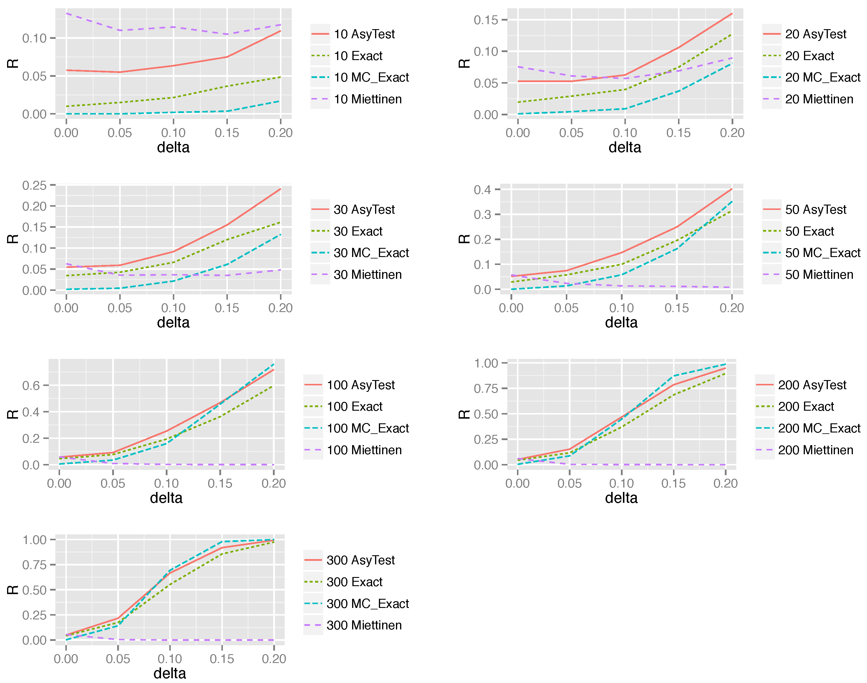
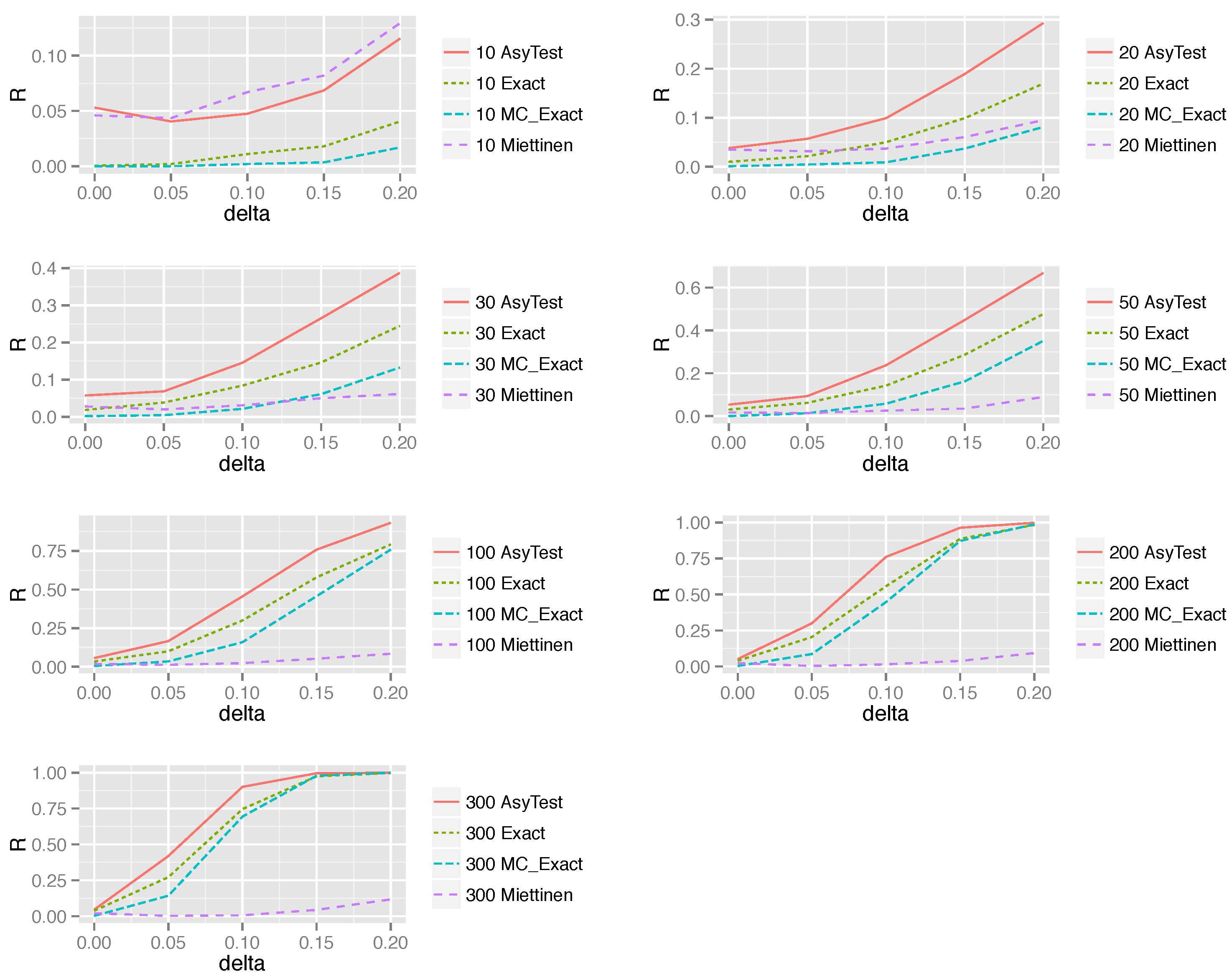
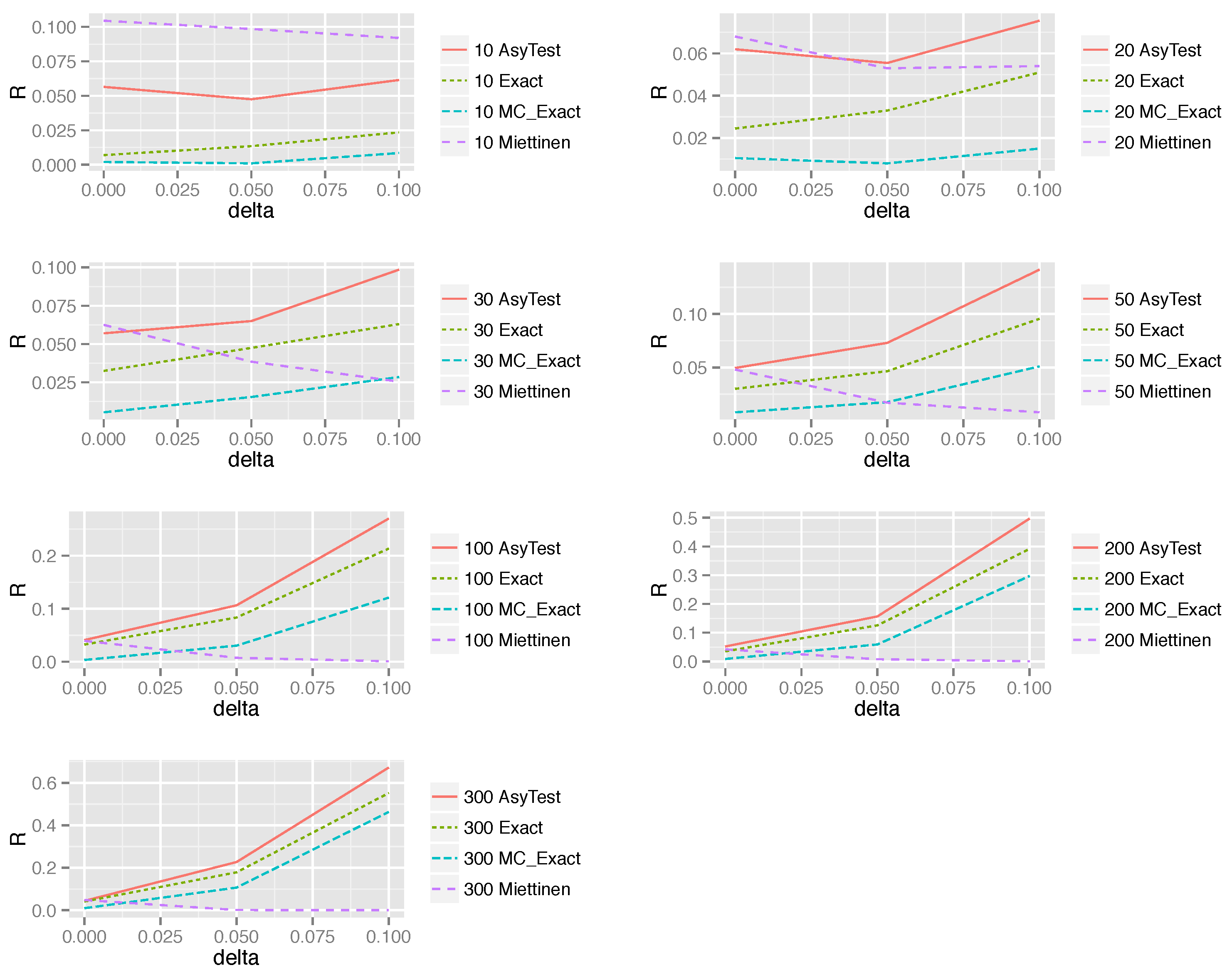
5. Simulation
5.1. The Simulation Setting
5.2. Simulation Results
6. Application Examples
6.1. Dual Sample Pooling Test
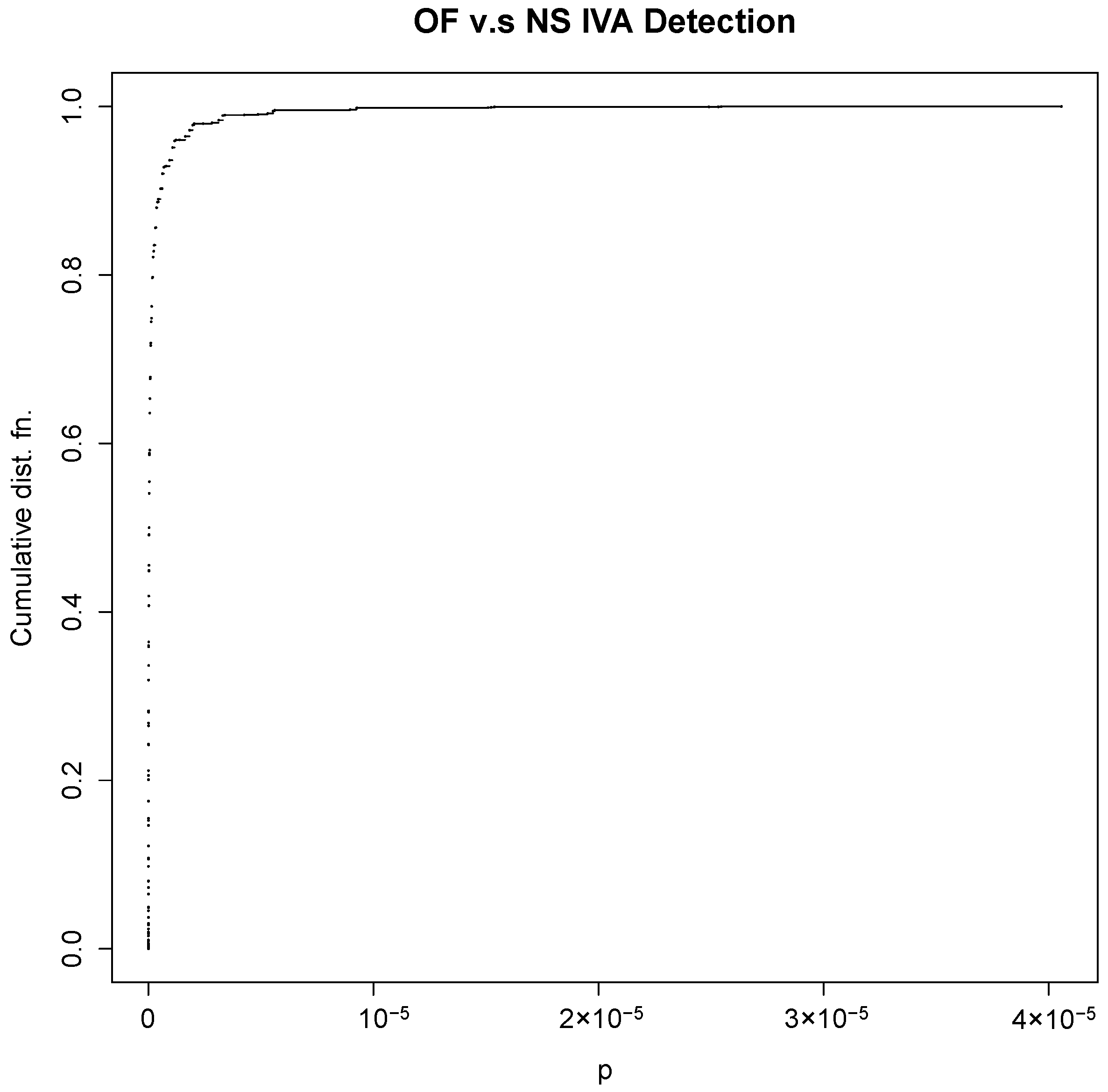
6.2. Pen-Based Oral Fluid Specimens for Influenza a Virus Detection
7. Discussion and Conclusions
Author Contributions
Funding
Data Availability Statement
Conflicts of Interest
References
- Dorfman, R. The Detection of Defective Members of large Populations. Ann. Math. Stat. 1943, 14, 436–440. [Google Scholar] [CrossRef]
- Litvak, E.; Tu, X.M.; Pagano, M. Screening for the Presence of a Disease by Pooling Sera Samples. J. Am. Stat. Assoc. 1994, 89, 424–434. [Google Scholar] [CrossRef]
- Zenios, S.A.; Wein, L.M. Pooled testing for hiv prevalence estimation: Exploiting the dilution effect. Stat. Med. 1998, 17, 1447–1467. [Google Scholar] [CrossRef]
- Tu, X.M.; Litvak, E.; Pagano, M. Studies of AIDS and HIV surveillance. Screening tests: Can we get more by doing less? Stat. Med. 1994, 13, 1905–1919. [Google Scholar] [CrossRef] [PubMed]
- Johnson, W.O.; Gastwirth, J.L. Dual group screening. J. Stat. Plan. Inference 2000, 83, 449–473. [Google Scholar] [CrossRef]
- Vansteelandt, S.; Goetghebeur, E.; Verstraeten, T. Regression Models for Disease Prevalence with Diagnostic Tests on Pools of Serum Samples. Biometrics 2000, 56, 1126–1133. [Google Scholar] [CrossRef] [PubMed]
- McNemar, Q. Note on the sampling error of the differences between correlated proportions of percentages. Psychometrika 1947, 12, 153–157. [Google Scholar] [CrossRef] [PubMed]
- Bennett, B.M.; Underwood, R.E. On McNemar’s test for the 2 × 2 table and its power function. Biometrics 1970, 26, 339–343. [Google Scholar] [CrossRef]
- Miettinen, O.S. Individual Matching with Multiple Controls in the Case of All-or-None Responses. Biometrics 1969, 25, 339–355. [Google Scholar] [CrossRef] [PubMed]
- Duffy, S.W. Asymptotic and Exact Power for the McNemar Test and Its Analogue with R Controls Per Case. Biometrics 1984, 40, 1005–1015. [Google Scholar] [CrossRef]
- Geyer, C.J.; Meeden, G.D. Fuzzy and Randomized Confidence Intervals and p-values. Stat. Sci. 2005, 20, 358–366. [Google Scholar] [CrossRef]
- Angulo, F.J.; Swerdlow, D.L. Epidemiology of Human Salmonella Enteric Server Enteritidis in the United States; Iowa State University Press: Ames, IA, USA, 1999. [Google Scholar]
- Patrick, M.E.; Adcock, P.M.; Gomez, T.M.; Altekruse, S.F.; Holland, B.H.; Tauxe, R.V.; Swerdlow, D.L. Salmonella enteritidis 364 infections, United States, 1985–1999. Emerg. Infect. Dis. 2004, 10, 1–7. [Google Scholar] [CrossRef] [PubMed]


| Diagnostic Testing Strategy 2 | |||||
|---|---|---|---|---|---|
| 2 | 1 | 0 | Total | ||
| Strategy 1 | 1 | ||||
| 0 | |||||
| Total | n | ||||
| Test 2 | |||||
|---|---|---|---|---|---|
| 2 | 1 | 0 | Total | ||
| Test 1 | 1 | 0 | 7 | 0 | 7 |
| 0 | 0 | 0 | 97 | 97 | |
| Total | 0 | 7 | 97 | 104 | |
| NS | |||||
|---|---|---|---|---|---|
| 2 | 1 | 0 | Total | ||
| OF | 1 | 114 | 28 | 29 | 171 |
| 0 | 2 | 7 | 42 | 51 | |
| Total | 116 | 35 | 81 | 222 | |
Disclaimer/Publisher’s Note: The statements, opinions and data contained in all publications are solely those of the individual author(s) and contributor(s) and not of MDPI and/or the editor(s). MDPI and/or the editor(s) disclaim responsibility for any injury to people or property resulting from any ideas, methods, instructions or products referred to in the content. |
© 2024 by the authors. Licensee MDPI, Basel, Switzerland. This article is an open access article distributed under the terms and conditions of the Creative Commons Attribution (CC BY) license (https://creativecommons.org/licenses/by/4.0/).
Share and Cite
Lin, H.; Zhu, A.; Wang, C. Statistical Tests for Proportion Difference in One-to-Two Matched Binary Diagnostic Data: Application to Environmental Testing of Salmonella in the United States. Mathematics 2024, 12, 741. https://doi.org/10.3390/math12050741
Lin H, Zhu A, Wang C. Statistical Tests for Proportion Difference in One-to-Two Matched Binary Diagnostic Data: Application to Environmental Testing of Salmonella in the United States. Mathematics. 2024; 12(5):741. https://doi.org/10.3390/math12050741
Chicago/Turabian StyleLin, Hui, Adam Zhu, and Chong Wang. 2024. "Statistical Tests for Proportion Difference in One-to-Two Matched Binary Diagnostic Data: Application to Environmental Testing of Salmonella in the United States" Mathematics 12, no. 5: 741. https://doi.org/10.3390/math12050741