Article

Persistent Homology Identifies Pathways Associated with Hepatocellular Carcinoma from Peripheral Blood Samples

by
Muhammad Sirajo Abdullahi
1,2,
Apichat Suratanee
3,4,
Rosario Michael Piro
5,† and
Kitiporn Plaimas
1,*,†
1
Advanced Virtual and Intelligence Computing (AVIC) Center, Department of Mathematics and Computer Science, Faculty of Science, Chulalongkorn University, Bangkok 10330, Thailand
2
Department of Mathematics, Faculty of Physical and Computing Sciences, Usmanu Danfodiyo University, Sokoto 840104, Nigeria
3
Department of Mathematics, Faculty of Applied Science, King Mongkut’s University of Technology North Bangkok, Bangkok 10800, Thailand
4
Intelligent and Nonlinear Dynamic Innovations Research Center, Science and Technology Research Institute, King Mongkut’s University of Technology North Bangkok, Bangkok 10800, Thailand
5
Dipartimento di Elettronica, Informazione e Bioingegneria, Politecnico di Milano, 20133 Milan, Italy
*
Author to whom correspondence should be addressed.
These authors contributed equally to this work.
Mathematics 2024, 12(5), 725; https://doi.org/10.3390/math12050725
Submission received: 22 January 2024 / Revised: 17 February 2024 / Accepted: 26 February 2024 / Published: 29 February 2024
(This article belongs to the Special Issue Advanced Computational Biology and Bioinformatics)

Abstract

:
Topological data analysis (TDA) methods have recently emerged as powerful tools for uncovering intricate patterns and relationships in complex biological data, demonstrating their effectiveness in identifying key genes in breast, lung, and blood cancer. In this study, we applied a TDA technique, specifically persistent homology (PH), to identify key pathways for early detection of hepatocellular carcinoma (HCC). Recognizing the limitations of current strategies for this purpose, we meticulously used PH to analyze RNA sequencing (RNA-seq) data from peripheral blood of both HCC patients and normal controls. This approach enabled us to gain nuanced insights by detecting significant differences between control and disease sample classes. By leveraging topological descriptors crucial for capturing subtle changes between these classes, our study identified 23 noteworthy pathways, including the apelin signaling pathway, the IL-17 signaling pathway, and the p53 signaling pathway. Subsequently, we performed a comparative analysis with a classical enrichment-based pathway analysis method which revealed both shared and unique findings. Notably, while the IL-17 signaling pathway was identified by both methods, the HCC-related apelin signaling and p53 signaling pathways emerged exclusively through our topological approach. In summary, our study underscores the potential of PH to complement traditional pathway analysis approaches, potentially providing additional knowledge for the development of innovative early detection strategies of HCC from blood samples.

1. Introduction

Primary liver cancer is one of the most common forms of cancer worldwide, with more than 905,000 new cases diagnosed and over 830,000 cancer-related deaths reported each year [1]. Hepatocellular carcinoma (HCC) is the most prevalent type of primary liver cancer accounting for over 75% of all cases, thus representing a significant global health concern [1]. One of the major challenges in HCC diagnosis is the lack of noticeable symptoms in the early stages of the disease, often leading to patients being diagnosed only when the disease has reached an advanced stage [2].
Diagnosing HCC and predicting treatment responses can be achieved using various biomarkers [3]. The World Health Organization (WHO) defines a biomarker as “any substance, structure or process that can be measured in the body or its products and [that can] influence or predict the incidence of outcome or disease” [4]. The conventional biomarker for early HCC detection, α-fetoprotein (AFP), is no longer recommended due to its limited sensitivity and specificity [5,6]. While newer biomarkers like des-γ-carboxy-prothrombin (DCP), osteopontin, interleukin-6 (Il-6), and Golgi protein 73 (GP73) have shown promise, none have achieved sufficient sensitivity or specificity [7]. Combining multiple biomarkers is a current approach showing potential to enhance HCC detection and monitoring [3]. Nevertheless, there is still room and a need for more accurate and reliable biomarkers for effective HCC prognosis, diagnosis, and treatment. This is especially true at the level of functional pathways involving many genes, which still poses a challenge in current research.
Topological data analysis (TDA) is a modern interdisciplinary field that combines algebraic topology, computational geometry, and statistical learning to analyze large volumes of high-dimensional data and extract relevant information [8]. It offers advantages such as independence from the choice of metric, robustness against noise, and a qualitative approach to understanding the ‘shape’ of data [9,10]. It can also integrate and visualize multidimensional data, potentially providing a better understanding of relationships between clinical samples where traditional data analysis methods may fall short [11].
TDA has proven to be a versatile tool across diverse applications, including digital data classification [12], multidimensional data derived from magnetic resonance imaging (MRI) scans of osteoarthritis patients [13], and the integration of computed tomography (CT) and MRI scans with clinical data from patients with traumatic brain injury [14]. Its efficacy extends to the analysis of mammogram scans/images [15,16] and it has demonstrated utility in genomics, particularly in the analysis of DNA copy number aberrations [17]. In the realm of infectious diseases, TDA has been applied to whole-blood RNA sequencing (RNA-seq) gene expression data [18] and to measurements of inflammatory biomarkers in blood plasma [19] from coronavirus disease 2019 (COVID-19) patients. A TDA-based approach also demonstrated its capability to distinguish idiopathic pulmonary fibrosis from multiple other diseases based on peripheral blood mononuclear cell (PBMC) gene expression data [20].
In short, TDA holds immense potential as a reliable tool for analyzing multidimensional data, such as gene expression levels obtained by RNA-seq. However, a specific implementation applying this method to functional pathways in order to capture topological changes based on the set of genes involved in a functional pathway is still lacking. To address this, our research utilizes persistent homology (PH) to identify significant pathways as potential prognostic biomarkers.
Figure 1 visually outlines our research pipeline, illustrating the process of evaluating alterations in genome-wide correlation of gene expression levels between control and disease sample classes. With this approach, we first identify a set of topological descriptors that show significant changes between HCC samples and normal controls. Then, we apply this pipeline to multiple pathway-specific subsets of genes to assess changes in the correlation of gene expression specifically within these pathways, mirroring the evaluation conducted on the full (genome-wide) gene expression data. Thus, we identify those cellular pathways that reflect the global changes in HCC samples as potential biomarker pathways. In addition to the pipeline sketch in Figure 1, we have included Algorithm 1 in Section 3 to further enhance the presentation of our proposed method.
In the case of analyzed HCC expression data from peripheral blood, taken from a study by Han et al. [21], we hypothesized that PH could facilitate early HCC detection by identifying such potential biomarker pathways. Specifically, we analyzed RNA-seq gene expression data from PBMCs of both HCC patients and normal controls, with 17 samples in each class. For each class, we first mapped the gene expression profile of each sample to a multidimensional space to form a point cloud. Then, we utilized PH to explore various topological descriptors associated with a persistence diagram in order to extract relevant features from the shape of the point cloud. Finally, we compared the descriptors obtained from the two sample classes to identify relevant differences.
Our analysis unveiled several significant cellular pathways whose expression patterns differ between peripheral blood from HCC patients and that from healthy controls. We evaluated our findings by conducting a comparative assessment with the frequently used enrichment-based pathway analysis, revealing pathways that were common or unique to both methods. The literature support and discussion of our results clearly demonstrate the benefit of PH for detecting functional pathways. Our findings reveal that previously unidentified pathways can be uncovered through the application of TDA using PH, and a set of key topological descriptors that effectively capture changes in gene expression between healthy and disease samples can be defined. This approach proves to be a promising tool that can be applied to other datasets and diseases, hopefully contributing to a deeper understanding of the complexities inherent in biological data and systems.
With this study, and the application of TDA for the identification of disease-associated pathways, we intend to address a major limitation of the most commonly used pathway analysis strategies: the assumption that alterations in the biological activity of a pathway depend on the overexpression or underexpression of a significant number of the genes involved in the pathway. However, for both signaling pathways and metabolic pathways, the output can depend on other factors such as coordinated feedback and timing [22,23,24].
We hypothesized that such effects could be better captured by TDA rather than an enrichment analysis approach based on differential expression of individual genes, and thus TDA might offer additional clues for pathway analysis, complementing traditional approaches rather than replacing them.
This motivated our exploration of TDA, specifically PH, to identify key pathways associated with HCC from peripheral blood samples. Our aim is to demonstrate how PH can provide valuable insights into intricate patterns and relationships in complex biological data, particularly in the context of HCC. By analyzing RNA-seq data, we seek to bridge gaps in current pathway analysis approaches.
The results of this pilot study showcase that PH-based methods can complement traditional pathway analysis approaches and provide a promising tool that could be applicable to various datasets and diseases, thus contributing to a deeper understanding of complexities inherent in biological data and systems. Our key contributions include the application of PH to analyze RNA-seq data from peripheral blood samples, the identification of topological descriptors capable of capturing changes in gene expression between healthy and disease samples, the identification of significant cellular pathways distinguishing HCC and healthy samples which include pathways known to be associated with HCC, such as the apelin signaling pathway, the IL-17 signaling pathway, and the p53 signaling pathway, as well as previously unidentified pathways. In addition, comparative analysis with the frequently used enrichment-based pathway analysis method reveals pathways that are common or unique to both methods, which underscores that they can be considered as complementing each other.
The paper is structured as follows: this section described the biomedical context and the objectives of the study. In Section 2, we present a basic introduction to topological data analysis. Section 3 details the materials and methods employed in the study. In Section 4, our results are presented, followed by a discussion in Section 5. Finally, Section 6 encompasses the conclusions and future research directions.

2. Topological Data Analysis: Background

In this section, we will provide a brief overview of homology (in the mathematical sense of topology, not biology or evolution) and persistent homology. For detailed formal definitions and further mathematical terms, please refer to Appendix A.

2.1. Simplicial Complex and Homology

Topology is a mathematical discipline that explores the structural relationships and connections between various regions within a space, similar to observing individual points or composed objects and determining how they are connected and what makes them different from one another. Having in mind a rubber sheet that can be stretched and deformed, but not torn or punctured, topology can be used for understanding which shapes can be transformed into one another through stretching without breaking [25]. TDA builds on these concepts to decipher the essential features of a dataset, even if it is composed of a limited set of data points. It thus helps to determine key characteristics of a complex shape using just a few points.
Homology is a mathematical technique that utilizes algebra to study the complex shapes of objects, starting from simple building blocks called k -simplices (like points, lines, triangles, and more), as illustrated in Figure 2. These blocks are assembled to create more complex shapes, like networks.
Usually, specific nomenclature is used to refer to the k -simplices of the lowest dimensions, k : “vertex” (point) for a 0-simplex, “edge” (two points joined by a line) for a 1-simplex, “triangle” (three points with joining edges and their enclosed space) for a 2-simplex, and “tetrahedron” (a solid triangular pyramid) for a 3-simplex (see Figure 2).
Simplicial complexes are systematic collections of these building blocks, as illustrated in Figure 3a–c. The dimension of a simplicial complex is the maximum dimension of any of its building blocks (simplices). For example, a network can be considered as a 1-dimensional simplicial complex with nodes (points, k = 0 ) and edges (lines, k = 1 ).
Various approaches are available for constructing simplicial complexes from initially unconnected data points, such as those we obtain when considering each sample as a point in a multidimensional space (see Section 3.1). We will use the Vietoris–Rips (VR) [25] complex method, which is commonly preferred in PH calculations for TDA due to its computational advantages. Essentially, the VR method assembles data points into higher-order objects if balls (circles) of a given threshold radius r , centered at the data points, overlap each other: i.e., their pairwise distances do not exceed 2 r , as illustrated in Figure 3d. For more details and an alternative method, see Appendix A.
Some key characteristics of simplicial complexes can be expressed by means of a set of topological invariants called Betti numbers. The k -th Betti number of a simplicial complex K is denoted as β k ( K ) , with k = 0 measuring the number of 0-dimensional holes (connected components), k = 1 measuring the number of 1-dimensional or “circular” holes (1-cycles), and k = 2 measuring the number of 2-dimensional holes (“cavities” or “voids”). A formal definition of β k ( K ) is provided in Appendix A.
The “holes” (of different dimensions) measured by these Betti numbers—i.e., the connected components, the circular holes, and the cavities—are referred to as “topological features” of a simplicial complex.

2.2. Persistent Homology

For a point cloud representing a set of data points in a high-dimensional space, classical homology, as outlined above, fails to give meaningful information. This limitation arises because when constructing simplicial complexes from individual data points, a dataset’s topology can vary significantly depending on the choice of the distance threshold parameter r , as can be seen in Figure 3d. Thus, determining a single representative threshold for the entire dataset can be a challenging or even an impossible task. To address this issue, the PH method offers an alternative approach.
Indeed, PH considers multiple or all values of the thresholding parameter r . As r increases, initially disconnected simplices can merge to form new, larger simplices (like edges formed from individual data points). These new simplices are then added to the current simplicial complex, resulting in a sequence of subcomplexes known as a “filtered simplicial complex” (see Figure 3d and Appendix A for more details).
PH involves tracking when (i.e., at what threshold parameter r ) new topological features (e.g., circular holes) emerge (referred to as ‘birth’) and when they disappear (referred to as ‘death’) by recording the corresponding distance thresholds r . This process captures how the topological properties of the complexes evolve as r increases.
Various methods in computational topology allow the summary and visualization of PH and multi-scale topological features, including persistence barcodes [26], persistence diagrams [27,28], persistence landscapes [29,30], persistence images [31], and persistence curves [32], each offering insights into data topology for different applications. In Figure 4, we provide an illustrative example for a given point cloud (Figure 4a).
Both persistence barcodes (Figure 4b) and persistence diagrams (Figure 4c) offer a clear representation of the lifespan (persistence) of each feature. Essentially, a persistence barcode portrays each feature as a bar, with the length of the bar reflecting the feature’s lifespan, while a persistence diagram visually represents each topological feature as a point on a graph, with the x - and y -axes denoting the distance threshold parameter r at the feature’s birth and death, respectively. In both visualization techniques, the color of the bar (in the persistence barcode) or point (in the persistence diagram) can indicate the dimension k of the corresponding topological feature.
Longer bars in the persistence barcode (or points located farther from the diagonal in the persistence diagram) are typically considered robust features of the dataset, while shorter bars in the persistence barcode (or points near the diagonal in the persistence diagram) are often interpreted as noise or less significant features [9]. Thus, PH is robust against data noise, making it a stable representation, where small perturbations in the data have only a minor effect on the barcode or persistence diagram.
Additionally, the evolution of Betti numbers as r increases can be visualized as Betti curves (see Figure 4d). For example, consider the topological features shown at three thresholds: r = 0.25 ,   r = 0.375 , and r = 0.5 . At r = 0.25 ,     β 0 = 6 , because there are only six connected components; the two closest points at the bottom left corner of Figure 4a have merged into one connected component, while β 1 = 0 due to the absence of 1-dimensional circular holes, i.e., 1-cycles (see also Figure 3d, third panel). At r = 0.375 ,     β 0 = 4 , because there are only four connected components; the three closest points at the top right corner of Figure 4a have merged into one connected component, while β 1 = 0 because there still is no 1-cycle (see also Figure 3d, fourth panel), whereas at r = 0.5 ,     β 0 = 1 ,   because the threshold radius   r   is large enough to merge all points into a single connected component, while β 1 = 1 due to the presence of a 1-cycle (see also Figure 3d, last panel).

3. Materials and Methods

As the research pipeline was previously outlined in Figure 1 and a more detailed implementation provided in Algorithm 1. Detailed information about the expression and pathway datasets used, the topological descriptors explored, and the methods employed in this study are explained in this section.
Algorithm 1: Persistent Homology Analysis of Gene Expression Data
Input:
  •  
    • Gene expression dataset (control and disease samples).
Output:
  •  
    • Persistence diagrams, persistence barcodes, and Betti curves.
    • Significant topological descriptors indicating differences between sample classes.
    • Significant KEGG pathways exhibiting topological changes similar to those observed for the genome-wide gene expression dataset.
  • PartitionDataset(GeneExpressionDataset)
    i.
    Separate the gene expression dataset into control (healthy) and disease (HCC) sample classes.
  • For each sample class:
    • ConstructPointCloud(GeneExpressionClass)
      i.
      Create a multidimensional point cloud, where each point represents the gene expression levels of a specific sample from the GeneExpressionClass.
      ii.
      Measure distances between points (samples) based on correlation coefficients.
    • ComputePersistentHomology(PointCloud)
      i.
      Identify persistent features using the point cloud.
      ii.
      Generate persistence diagrams and persistence barcodes representing birth and death of topological features.
    • ExtractTopologicalDescriptors(PersistenceHomology)
      i.
      Measure all the topological descriptors defined in Section 3 from the persistence homology computed for the sample class.
  • AssessDifferences(TopologicalDescriptorsControl, TopologicalDescriptorsDisease)
    i.
    Randomly permute the class labels of the samples and recompute topological descriptors (steps 1 and 2). Perform this random permutation 2000 times to obtain a distribution of random values for each topological descriptor.
    ii.
    Compare the observed/actual values of each descriptor with their corresponding values obtained from permuted/randomized class labels to determine statistical significance.
  • IdentifySignificantDescriptors(TopologicalDescriptor)
    i.
    Identify topological descriptors showing significant differences between control and disease classes.
  • ApplyWorkflowToSubsets(GeneExpressionDataset, PathwaySubsetGeneSets)
    i.
    For the pathway-specific analysis, the focus is on subsets of genes associated with each particular pathway.
    ii.
    Apply steps 1–4 above to each KEGG pathway gene set, limiting the gene expression dataset to the subset of genes involved in the given pathway.
    iii.
    Identify pathways where the topological descriptors, specifically those that showed significance in the genome-wide gene expression dataset at step 4, also demonstrate significance.

3.1. PBMC Gene Expression Data

Gene expression dataset. The data were obtained from a study by Han et al. [21], which employed RNA-seq to profile gene expression patterns in PBMC from 17 patients with hepatocellular carcinoma and 17 healthy controls of similar age. Of 30,474 genes with discernible gene expression levels in the PBMC samples, as selected by the original authors, we used only those 26,575 genes that have a corresponding HGNC gene symbol.
RNA-seq data were generated by Han et al. based on the following experimental technique: RNA transcripts (molecules) extracted from cells are converted to their DNA equivalent and subsequently fractured into smaller pieces which are sequenced. The obtained sequence “reads” are then aligned/mapped to the reference genome or transcriptome. Since the number of RNA transcripts of a gene present in the cells determines the number of obtained sequence reads for that gene, gene expression levels can be estimated from the number of reads which map to the corresponding genomic regions.
Data pre-processing and normalization. As suggested by a recent validation by Abrams et al. [33], we employed the Transcripts Per Million (TPM) method [34] to normalize the RNA-seq gene expression data using ‘edgeR’ [35] (R package version 3.42.4, R version 4.3.0). Afterwards, a log2 transformation was carried out on the resultant TPM values.
Data representation for genome-wide gene expression. Each sample was treated as a data point (sample vector) within a 26,575-dimensional space, defined by the expression levels of the individual genes in that sample. Thus, the set of HCC or control samples form a ’point cloud’ to which PH can be applied.
Data representation for pathway-specific gene expression. For gene sets from individual cellular pathways, we essentially used the data representation in a point cloud but defined each data point (sample vector) only by the expression levels of the genes involved in each pathway, thus reducing the 26,575-dimensional space to an N -dimensional space, where N is the number of genes involved in the pathway.
Distance metric. To measure the distances between samples, i.e., between the data points in the point cloud, different distance metrics can be used, such as the Euclidean distance or a distance based on a correlation coefficient. In biomedical research, the similarity (or dissimilarity) of samples is usually measured in terms of the positive (or negative) correlation of their gene expression profiles. Therefore, we defined the distance between two samples as 1 ρ , where ρ is the Pearson correlation coefficient between the samples. Since ρ can range from −1 (perfect anti-correlation) to 1 (perfect correlation), the distance can theoretically range from 0 to 2.

3.2. KEGG Pathways

We obtained a list of cellular pathways and their associated genes from the Kyoto Encyclopedia of Genes and Genomes (KEGG) [36] database using the R (version 4.3.0) packages, ‘AnnotationDbi’ (version 1.62.2), and ‘org.Hs.eg.db’ (version 3.17.0). For our study, we focused exclusively on the 251 metabolic pathways and signaling pathways.

3.3. PH Implementation

In this study, we employed PH as the chosen topological method. We categorized the gene expression dataset into two classes consisting of control samples only and disease samples only, and applied PH to both classes individually. We constructed the VR complexes from the corresponding sample point clouds, using the distance metric defined above. The Python version of ‘Gudhi’ [37] (version 3.7.1) (https://gudhi.inria.fr/ (accessed on 20 December 2023)) was used for the computation of PH and for generating our visualizations.

3.4. Topological Descriptors

Let k represent the dimension of a k -simplex in an n -dimensional simplicial complex. We defined several key descriptors for the topological features in our analysis. Specifically, m k represents the count of k -dimensional topological features, b i , k denotes the “birth time” of the i -th k -dimensional feature (threshold radius r at which the feature appears), d i , k denotes the “death time” of the i -th k -dimensional feature ( r at which the feature ceases to exist), and p l k corresponds to the total (summed) persistence (lifetime) of all features of dimension k . The topological descriptors we consider for our analysis are explicitly defined as shown in Table 1. It is worth noting that most of these descriptors apply to topological features ( k -cycles) of specific dimension k within a persistence diagram. Only two descriptors, namely the classical and persistence-wise Euler characteristics, take into account the contribution of topological features ( k -cycles) across all possible dimensions (e.g., connected components, 1-cycles, cavities, etc.).
It is important to highlight that a value of zero for a topological descriptor of dimension k typically indicates the absence of features in that particular dimension. Exceptions to this are Classical EC and Persistence EC, where a value of zero does not necessarily indicate the absence of features due to the involvement of multiple dimensions in their computation.

3.5. Differential Expression Analysis

For the classical approach to pathway analysis, differential expression analysis was performed using the ‘PyDESeq2’ [38] package (version 0.4.4) for Python (version 3.10.7). Only genes with an adjusted p -value < 0.05   (adjusted for multiple testing using the Benjamini–Hochberg method) and a log fold change 1 were considered as significantly differentially expressed.

3.6. Enrichment Analysis of Pathways

The classical enrichment-based pathway analysis was carried out using the ‘Scipy’ [39] package (version 1.10.1) for Python (version 3.10.7). Essentially, it performs a hypergeometric enrichment test (one-sided Fisher’s exact test) to identify pathways containing a significantly high number of differentially expressed genes. For each pathway, it calculates a p -value, which in essence is the likelihood of observing at least m differentially expressed genes in a pathway purely by chance, considering the total number of genes in the dataset, the total number of genes in the pathway, and the total number of differentially expressed genes. p -values were corrected for multiple testing (251 pathways) using the Benjamini–Hochberg method.

3.7. Significance of Topological Descriptors

To assess whether topological descriptors of the PH-based approach differ significantly between sample classes, we performed a two-tailed statistical permutation test using Python (version 3.10.7) and the Benjamini–Hochberg correction of p -values for multiple testing using the ‘Statsmodels’ [40] package (version 0.13.5). Essentially, 2000 random permutations of the sample labels were generated, and there were correspondingly 2000 random assignments of samples to the disease and control classes.
For each of the permutations, we applied PH and computed the values of the topological descriptors individually for the two sample classes. For each topological descriptor TD, we computed the difference between disease and control samples as: TD(disease)—TD(control). We repeated this entire process for all 2000 permutations to build a distribution of differences under the null hypothesis that there is no association (or biological distinction) between the peripheral blood samples of the two classes.
To quantify significance, for each descriptor, we calculated the empirical or permutation p -value, which measures the proportion of random permutations that yield a more extreme value (in either direction) than the observed (actual) value. Subsequently, to account for multiple testing, we applied the Benjamini–Hochberg procedure, which resulted in adjusted p -values. These adjusted p -values help control the false discovery rates (FDR), indicating the likelihood of false discoveries (incorrectly identifying differences) and potential for false positives (attaining statistically significant results by chance) among the descriptors. Throughout our analysis, we set the FDR threshold to be less than 0.05.

4. Results

4.1. Genome-Wide Persistent Homology Analysis

Initially, we leveraged the full (genome-wide) HCC RNA-seq gene expression dataset from the study by Han et al. [21] (see Section 3 for details) to identify key topological descriptors that effectively capture changes in genome-wide gene expression between 17 HCC samples and 17 healthy controls.
The process, outlined in Figure 1 and Algorithm 1, begins by partitioning the genome-wide gene expression data into datasets for control and disease samples. PH is then individually applied to each class.
For each sample class, the genome-wide gene expression levels of each individual sample are represented as a data point in the input point cloud, used for the construction of the VR complexes and the computations of their persistent homologies. Distances between data points are measured based on the Pearson correlation coefficient between the corresponding samples, as detailed in Section 3.1. Subsequently, topological descriptors for both sample classes were derived from the persistence diagrams obtained through PH calculations (see Section 3.4 for details about each descriptor). To visualize the topological (homological) evolution resulting from the computation of PH, we created and plotted persistence barcodes, persistence diagrams, and Betti curves for each class (see Figure 5).
We noticed that the most persistent features were the 0-dimensional features (i.e., connected components). This observation remains valid irrespective of whether the data were from the control class or the disease class. Additionally, 1-dimensional topological features (i.e., 1-cycles/circular holes) and 2-dimensional topological features (i.e., 2-cycles/voids) were also present although not as persistent as the 0-dimensional topological features. No 3-dimensional topological features (3-cycles) were detected, which allowed us to omit the calculation of topological features of higher dimensions (3 and above), resulting in a substantial reduction in computation time without compromising the quality of the output represented by the computed topological descriptors. In addition, we observed that since most of the 1-dimensional and 2-dimensional topological cycles were not very persistent (had short lifespans), the value of Persistence EC was very close to that of Sum P-0 (see Table 2 and Supplementary Table S1).
We then assessed through a permutation test whether the computed values of a topological descriptor significantly differed between disease and control samples. To achieve this, we first computed the values of all the considered topological descriptors for both classes and then determined the difference between the two classes for each descriptor (see Section 3.7). These differences served as our measure of the global changes in gene expression observable in HCC peripheral blood samples with respect to controls.

4.2. Choice of Relevant Topological Descriptors

To identify the subset of topological descriptors that best reflect genome-wide gene expression changes in HCC samples, we performed a two-tailed permutation test on the sample labels (random assignment of samples to disease and control classes) to evaluate the statistical significance of the observed differences in topological descriptors between peripheral blood from HCC patients and healthy controls.
Several of the topological descriptors showed highly significant differences (FDR below 0.05) between control and disease samples (see Table 2 and Figure A3, as well as Supplementary Table S1 and Figure S1 for additional details). Specifically, we have identified the persistence-wise Euler characteristic (Persistence EC), the sum of persistence of 0-dimensional features (Sum P-0), the average persistence of 0-dimensional features (Average P-0), the range of persistence of 2-dimensional features (Range P-2), the sum of birth times of 2-dimensional features (Sum BT-2), and the sum of death times of 2-dimensional features (Sum DT-2) as the descriptors meeting our statistical significance criteria. Hence, we selected them as representative of the differences in peripheral blood between HCC patients and healthy controls.
Furthermore, we made noteworthy observations regarding these descriptors. Specifically, we found that Persistence EC, Sum P-0, and Average P-0 exhibited higher values in the disease class compared to the control class, while Range P-2, Sum BT-2, and Sum DT-2 had higher values in the control class because topological features of the dimensions k = 2 are not present in the PH of the disease class. The observation of higher values for topological descriptors in dimension k = 0 (namely, Sum P-0 and Average P-0) indicates a greater sample heterogeneity in the disease class compared to the control class, similar to what has been observed for autism spectrum disorder in a previous study [41].
In summary, we identified a subset of six topological descriptors (see Table 2) that best reflect genome-wide gene expression changes in peripheral blood from HCC patients.

4.3. Classical Differential Gene Expression Analysis and Enrichment-Based Pathway Analysis

Before using our new PH-based approach for pathway analysis, we applied the most frequently used classical pathway analysis method, so that we would be able to compare our results to those which can be obtained using a standard approach.
First, we used the genome-wide expression data and identified 1426 differentially expressed genes (adjusted p -value (FDR) of less than 0.05 and log-fold change of at least 1). Among these significantly dysregulated genes, 1242 genes were up-regulated, while 184 genes were down-regulated in peripheral blood of HCC patients (see Supplementary File S2 for details).
Afterwards, we assessed the significance of 251 KEGG metabolic pathways and signaling pathways by performing a hypergeometric enrichment test (one-sided Fisher’s exact test; see Section 3) to identify pathways containing a significant number of differentially expressed genes. Only sixteen pathways exhibited a significant enrichment in differentially expressed genes with an adjusted p -value (FDR) of less than 0.05 (see Supplementary Table S2 for details).

4.4. Persistent Homology Analysis for Pathway-Specific Gene Sets

Subsequent to the selection of six topological descriptors indicative of genome-wide gene expression patterns in peripheral blood from HCC patients, we investigated whether there are specific cellular pathways which reflect these global changes, hypothesizing that such pathways might potentially aid in an early detection of HCC from peripheral blood.
To this end, we applied our PH pipeline to various subsets of genes involved in specific cellular pathways, taking only the corresponding gene expression data instead of the full (genome-wide) dataset. That is, using functional gene sets for 251 metabolic pathways and signaling pathways from the KEGG database [36], we applied essentially the same methodology that we had used for the genome-wide gene expression dataset (see above) to focus only on the expression levels of the sets of genes involved in individual KEGG pathways to define the sample data points in the point cloud (see Section 3.1).
Our primary objective here was to assess the significance of pathways based on whether the previously identified topological descriptors showed significant differences between HCC samples and control samples—limited to the gene expression of the corresponding pathway gene sets—because we reasoned that those pathways which yield significant changes for the same topological descriptors would best reflect the genome-wide differences between HCC samples and those from healthy controls.
First considering individual topological descriptors, we observed that Persistence EC and Average P-0 detected the same set of pathways (138 pathways), while Sum BT-2 and Sum DT-2 produced identical results (36 pathways). In addition, Sum P-0 identified 137 pathways and Range P-2 identified 181 pathways, respectively (see Supplementary File S1 for a detailed list).
Visualizations in Figure 6 illustrate the number of pathways for which the individual topological descriptors show significant differences between HCC samples and controls, as well as the overlap of these sets of pathways with the 16 pathways identified as enriched in differently expressed genes.
Since our purpose is to identify pathways that best reflect the genome-wide changes in gene expression, instead of considering pathways with respect to individual topological descriptors, we define a pathway as significant when it exhibits significant changes across all six topological descriptors, mirroring the observations made for the genome-wide gene expression dataset. This criterion was met by twenty-three pathways, as illustrated in Figure 7a and detailed in Table 3.
It is important to note that for 2-dimensional features (cavities or voids), the associated topological descriptors can also be significant if their difference between HCC samples and controls is zero, indicating that these features are absent in the PH of both types of samples. When randomizing sample classes, instead, these features can appear and thus lead to a non-zero difference, such that a zero difference obtained with the correct sample classes may indeed be statistically significant.
The pathways identified as relevant by our PH method include genetic information processing pathways (RNA polymerase, protein processing in endoplasmic reticulum, and base excision repair), environmental information processing pathways (ABC transporters and apelin signaling pathway), a cellular process pathway (p53 signaling pathway), organismal system pathways (IL-17 signaling pathway and collecting duct acid secretion), and several metabolic pathways (riboflavin metabolism, citrate/TCA cycle, sulfur metabolism, ascorbate and aldarate metabolism, drug metabolism—cytochrome P450, glycine, serine and threonine metabolism, primary bile acid biosynthesis, phosphonate and phosphinate metabolism, histidine metabolism, tryptophan metabolism, beta-alanine metabolism, pantothenate and CoA biosynthesis, and porphyrin metabolism); refer to Table 3 for additional details.

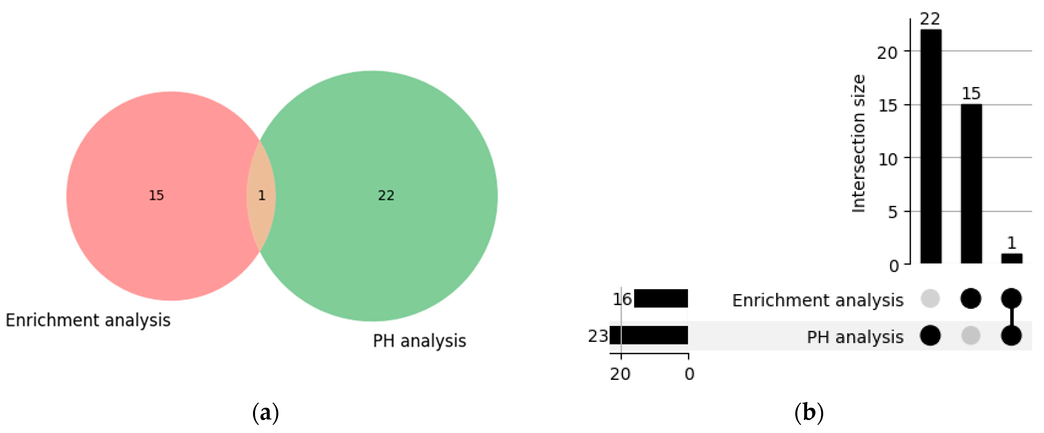
4.5. Comparison of Pathways Identified by the PH Method and the Enrichment Analysis

We compared our novel approach with the commonly used enrichment-based pathway analysis method, which identifies significant pathways through the hypergeometric enrichment test of differentially expressed genes in a pathway. Notably, our results revealed mostly unique significant pathways obtained by these approaches.
Among the 23 significant pathways detected by our PH method, only the IL-17 signaling pathway was also identified by the classical enrichment-based method (see Figure 8). Remarkably, 22 pathways were unique to our PH method (see Figure 8). Although these pathways did not show a significant enrichment in differentially expressed genes, they provide valuable insights into the molecular processes that may help to detect HCC from peripheral blood samples, deserving further investigation, experimental validation, and functional studies. Similarly, the pathways uniquely identified by the hypergeometric enrichment test (see Supplementary File S1 and Table S2 for details) but not detected by our PH method should not be disregarded.
Interestingly, several pathways identified by our PH method have been previously associated with HCC, or their association has been suggested by other computational approaches. For completeness, we provide a list: genetic information processing pathways (RNA polymerase [42], protein processing in endoplasmic reticulum [43], and base excision repair [44,45]), environmental information processing pathways (ABC transporters [46,47,48] and apelin signaling pathway [49,50]), a cellular processes pathway (p53 signaling pathway [51,52,53,54]), organismal systems pathways (IL-17 signaling pathway [55,56] and synaptic vesicle cycle [57]), and several metabolism pathways (riboflavin metabolism [58], citrate/TCA cycle [59,60,61], ascorbate and aldarate metabolism [62,63], drug metabolism—cytochrome P450 [48,64,65,66,67], glycine, serine, and threonine metabolism [48,64,68], primary bile acid biosynthesis [64], histidine metabolism [64], beta-alanine metabolism [64], tryptophan metabolism [54,64,69,70], pantothenate and CoA biosynthesis [58,71,72,73], and porphyrin metabolism [58,74,75]). This suggests that our method may indeed be capable of detecting subtle, HCC-related changes from peripheral blood.
Fifteen pathways were enriched in differentially expressed genes but not detected as significant by our PH method (see Figure 8). These include complement and coagulation cascades, the PPAR signaling pathway, hematopoietic cell lineage, the cholesterol metabolism, neutrophil extracellular trap formation, osteoclast differentiation, ECM–receptor interaction, platelet activation, cytokine–cytokine receptor interaction, neuroactive ligand–receptor interaction, the phagosome, fat digestion and absorption, the glycerolipid metabolism, the JAK-STAT signaling pathway, and the calcium signaling pathway (see Supplementary Table S2 for details).

5. Discussion

Detecting the presence of a severe disease such as HCC from the peripheral blood sample of an individual necessitates the identification of key biomarkers, be they specific metabolites, proteins, genes, or pathways. Unlike previous studies that primarily focused on applications of PH for tasks such as classification, prediction, or clustering [76,77,78], our study demonstrates the effectiveness of utilizing PH to explore the global characteristics of RNA-seq expression data from peripheral blood of both HCC patients and healthy individuals to identify significant pathways.
We first identified a set of topological descriptors that showed significant differences with respect to genome-wide expression data of HCC samples and normal controls. Persistence EC assesses the topological complexity of a pathway by examining persisting features across multiple dimensions during various stages of filtration, i.e., at various threshold radii r . Sum P-0, which is equivalent to the sum of death times of 0-dimensional features (connected components), provides insights into their persistence, reflecting the heterogeneity of gene expression between samples. Longer persistence indicates larger distances in the data point cloud and hence lower correlation between samples. Additionally, Average P-0 captures the mean persistence of 0-dimensional features. On the other hand, Range P-2, Sum BT-2, and Sum DT-2 elucidate the evolution of 2-dimensional features, emphasizing the birth, persistence, and demise of voids or cavities within the topology of the samples’ point cloud.
We then applied the PH method to pathway-specific gene expression data rather than genome-wide data, reasoning that pathways that reflect global changes may be particularly interesting as potential biomarker pathways. Among the twenty-three identified significant pathways, the IL-17 signaling pathway, also detected by the classical enrichment analysis method, is particularly noteworthy.
Figure 9 illustrates how pathways that were either identified as significant by our PH method, or were not evidenced as such, do or do not reflect patterns observed from genome-wide gene expression data.
HCC-related samples generally showed more heterogeneity than control samples. This is suggested by 0-Betti numbers β 0 , i.e., the numbers of connected components (but disconnected between each other), which decline much slower with increasing threshold radius r , indicating an overall lower pairwise correlation between samples.
The pathways identified as significant by our method displayed a pattern resembling more closely the genome-wide gene expression dataset (Figure 9a). Specifically, for significant pathways like the citrate cycle/TCA cycle (Figure 9b) and the p53 signaling pathway (Figure 9c), the 0-Betti numbers in the control class (blue curves) exhibited a sudden and faster drop than in the disease class (red curves), where the decline was more gradual. Conversely, pathways not identified by our method, such as the fructose and mannose metabolism (Figure 9d) and the phospholipase D signaling pathway (Figure 9e), showed a simultaneous but gradual decline phase for both sample classes. This observation suggests that topological features, such as the number of connected components, evolve differently as the radius increases.
For many of the 23 pathways highlighted by our method, we found indications for an experimentally validated or at least predicted association with HCC in the literature. The identified pathways, particularly those exclusive to our method, despite not being enriched in differentially expressed genes, offer a valuable resource for further exploration and experimental validation as biomarkers for peripheral blood. The importance of the p53 signaling pathway (see Figure 9c), for example, is supported both methodologically and biologically [51,52,53,54].

6. Conclusions and Future Research

Our study represents a pioneering effort in applying persistent homology (PH) analysis to identify tumor-associated pathways, particularly from PBMC samples of HCC patients. Analyzing RNA-seq data from peripheral blood, we successfully identified 23 significant pathways, including the apelin signaling pathway, the IL-17 signaling pathway, and the p53 signaling pathway. Our findings suggest that PH-based methods are complementary to classical enrichment-based pathway analysis methods and could thus be used in conjunction with current approaches to identify relevant pathways for experimental validation. We anticipate that applying our method directly to samples from affected disease tissues, rather than peripheral blood, could further advance our understanding of complex diseases.
While TDA methods, including PH, have shown promise in various applications, their use in gene expression analyses is still in its early stages and, to our best knowledge, ours is the first application to the pathway analysis problem. Looking ahead, future research could refine and expand the utility of TDA methods, particularly PH, by exploring their integration with other approaches for the comprehensive analysis of complex biomedical data. This approach holds the potential to advance our understanding of complex diseases and ultimately improve diagnostic strategies. The gained knowledge, e.g., about potential biomarker pathways, may ultimately help to develop early detection strategies that can be applied to individual samples or patients.

Supplementary Materials

The following supporting information can be downloaded at: https://www.mdpi.com/article/10.3390/math12050725/s1, File S1: List of pathways identified by persistent homology analysis through each individual topological descriptor and their overlaps; File S2: Results of differential gene expression analysis; Figure S1: Kernel density estimator (KDE) plots illustrating significance for all the topological descriptors considered; Table S1: Topological descriptors and their computed values for both control and disease sample groups, along with their differences, the p -values, and adjusted p -values for the genome-wide gene expression dataset; Table S2: List of pathways identified through the enrichment-based pathway analysis.

Author Contributions

For conceptualization, methodology, validation, formal analysis, and manuscript writing, M.S.A., A.S., R.M.P. and K.P.; software and visualization, M.S.A.; resources, M.S.A. and K.P.; data curation, M.S.A. and A.S.; supervision, A.S., R.M.P. and K.P.; funding acquisition, M.S.A., A.S. and K.P. All authors have read and agreed to the published version of the manuscript.

Funding

This research project is supported by the Second Century Fund (C2F), Chulalongkorn University. Apichat Suratanee was funded by the National Science, Research and Innovation Fund (NSRF) and King Mongkut’s University of Technology North Bangkok with Contract no. KMUTNB-FF-66-08.

Data Availability Statement

The original sequencing data can be accessed at the National Center for Biotechnology Information (NCBI) under project PRJNA739257 (https://dataview.ncbi.nlm.nih.gov/object/PRJNA739257). Additionally, supplementary data analyzed in this study, along with the codes used for reproducibility, are available on our GitHub repository: https://github.com/DrMSAbdullahi/PBMC_RNASeqHCC_PH_Analysis.

Acknowledgments

The authors are thankful to the anonymous reviewers for their careful reading and valuable suggestions.

Conflicts of Interest

The authors declare no conflicts of interest.

Abbreviations

The following abbreviations are used in this manuscript:
FDRFalse discovery rate
HCCHepatocellular carcinoma
KEGGKyoto Encyclopedia of Genes and Genomes
PBMCPeripheral blood mononuclear cell
PHPersistent homology
RNA-seqRNA sequencing
TDATopological data analysis
TPMTranscripts per million
VRVietoris–Rips

Appendix A. Simplicial Complex and Homology

We begin with the definition of a k -simplex, which is the building block of a simplicial complex (see Figure 2 and Figure 3).
Definition A1. 
A k -simplex σ = [ u 0 ,   u 1 ,   ·   ·   ·   ,   u k ] is the convex hull of k + 1 affinely independent points. That is, the set of all convex combinations i = 0 k α i u i such that i = 0 k α i = 1 and 0 α i 1 for all i { 0 ,   1 ,   .   .   .   ,   k } .
By the definition above, the dimension of σ is k . We usually assign specific nomenclature for the initial dimensions: “vertex” (point) for a 0-simplex, “edge” (two points joined by a line) for a 1-simplex, “triangle” (three points with joining edges and their enclosed space) for a 2-simplex, and “tetrahedron” (a solid triangular pyramid) for a 3-simplex (see Figure 2). A simplex spanned by a proper nonempty subset of the vertex set of σ is called a face of σ . We write σ * σ if σ * is a face of σ .
Definition A2. 
A simplicial complex K is a finite union of simplices so that
  • for any simplex σ     K , all its faces must be in K ;
  • if σ = σ 1 σ 2 for any two simplices σ 1 ,   σ 2 K then either σ = or σ is a common face of σ 1 and σ 2 .
The conditions above imply that if σ is a simplex in K , then all its faces must also be in K and any two simplices in K that are not disjoint must share a common simplex that is also a face to both of them. See Figure 3a–c for examples of what is a simplicial complex and what is not. The dimension of a simplicial complex K is the maximum dimension of any of its simplices.
Many approaches exist for constructing simplicial complexes from a topological or metric space, e.g., from the individual points of a point cloud. We will mention only two commonly used approaches, starting with the C ˇ ech complex.
Definition A3. 
Let D be a finite set of simplices and r > 0 ; the C ˇ ech complex C ˇ is defined as:
C ˇ r D = { σ D : x σ B x ( r ) } ,
where B x ( r ) denotes a ball of radius r > 0 centered at x . Simply put, for each σ D ,   σ C ˇ r ( D ) if the set of all r -balls centered at points of σ has a nonempty intersection (see Figure A1a).
Another way of constructing simplicial complexes is the VR complex.
Definition A4. 
Let D be a finite set of simplices and r > 0 ; the Vietoris–Rips complex VR, is defined as:
V R r D = { σ D   : d i a m   σ 2 r } .
Simply put, for each σ D ,   σ V R r ( D ) if the diameter of σ is at most 2r, which implies that the data points of which σ is composed have pairwise distances that do not exceed the threshold 2 r (see Figure A1b).
Figure A1. Example for the construction of simplicial complexes for a given point cloud (see Figure 4a and first panel in Figure 3d): (a) C ˇ ech complex; (b) VR complex. Note: (b) is equivalent to panel 4 in Figure 3d.
Mathematics 12 00725 g0a1
For the VR complex at threshold (radius) r , a k -simplex is formed when k + 1 points are within a pairwise distance of at most 2 r from each other, connecting each pair of points with an edge. This is the same as demanding that each possible pair of balls with a radius of r centered around k + 1 points have an overlapping region. For example, a 2-simplex is formed when there are nonempty pairwise intersections among three balls, as shown in Figure A1b.
For the C ˇ ech complex, in contrast, a k -simplex is formed in case there is a nonempty intersection of all the   k + 1 balls surrounding its points. For example, a 2-simplex is formed when there is a nonempty intersection among the three balls. To illustrate the difference, note that in Figure A1a ( C ˇ ech complex), what appears to be a triangle is actually composed of three individual 1-simplices (edges), while in Figure A1b (VR complex), the triangle is indeed a 2-simplex because a pairwise intersection of the three r -balls is sufficient; an intersection of all three r -balls is not required. Note that the edges in the VR complex are the same as in the C ˇ ech complex, and the required threshold to form a triangle in the C ˇ ech complex is slightly larger than in the VR complex. Consequently, the C ˇ ech complex is a subcomplex of the VR complex, i.e., C ˇ r ( D )     V R r ( D ) . The C ˇ ech complex has been proven to have the same homology as the union of all balls of radius r centered around the data points [25]. However, this equivalence need not hold for the VR complex. The VR complex, on the other hand, has significantly lower memory requirements since only the edges need to be stored for its computation, while computing the C ˇ ech complex requires the identification of higher-order intersections of the r -balls.
Definition A5. 
Suppose that K is a d -dimensional simplicial complex. Let k     { 0 ,   1 ,   .   .   .   ,   d } and { σ 1 ,   σ 2 ,   .   .   .   ,   σ p } be the set of k -simplices of K . Then a k -chain is defined as:
c = i = 1 p λ i σ i ,   where   λ i Z / 2 Z = { 0 ,   1 } .
Since the coefficients are in Z / 2 Z , a k -chain can be interpreted geometrically as a finite assembly of k -simplices. The term ‘chain complex’ typically refers to the “space of k -chains” of a simplicial complex K , denoted as C k ( K ) . This space, C k ( K ) , is defined as the collection of elements that are finite sums of k -simplices from K . While k -chains encompass a wide range of linear combinations of k -simplices within K , it is important to note that k -cycles and k -boundaries are regarded as special cases of k -chains. Specifically, k -cycles represent closed chains (loops that do not have any ‘loose ends’), whereas k -boundaries correspond to the boundaries (edges) of ( k + 1 )-chains.
The boundary map k : C k ( K ) C k 1 ( K ) is a homomorphism satisfying the fundamental property k k + 1 = 0 . In simple terms, the boundary k of a k -simplex σ is usually denoted by k σ and defined as the sum of ( k 1 )-faces of σ . The kernel of k (Ker k for short), called the “space of k -cycles of K ”, is denoted by Z k ( K ) and defined as:
Z k ( K ) = { σ C k ( K )   : k σ = 0 } ,
and the image of k + 1 (Im k + 1 for short), called the “space of k -boundaries of K ”, is denoted by B k K and defined as:
B k ( K ) = { σ C k ( K )   :   t h e r e   i s   σ * C k + 1 ( K ) ,     k + 1 ( σ * ) = σ } .
In what follows, we present the formal definition of a simplicial homology group, which informally means a group containing cycles that are not boundaries.
Definition A6. 
The k -th simplicial homology group of a simplicial complex K is the quotient vector space defined as:
H k K = Z k K B k K .
The simplicial homology group serves as a container for cycles that are not mere boundaries. The concept is crucial in computing Betti numbers, such as β 0 ,   β 1 , and β 2 , which serve as robust measures for capturing topological features in data. These numbers offer valuable insights into the structure of the data by quantifying various topological characteristics, such as counting holes at different dimensions. For example, they can help identify the number of distinct clusters, circles, voids, or higher-dimensional holes present in the data.
The k -th Betti number of a simplicial complex K , denoted as β k ( K ) , is formally defined as the dimension of the k -th homology group, H k K (i.e., β k ( K ) = d i m   H k ( K ) . ) Importantly, it is well-established that both H k ( K ) and β k ( K ) are topological invariants. In other words, if we have two simplicial complexes, K and L , whose geometric realizations are homotopy equivalent, their homology groups must be isomorphic, and their corresponding Betti numbers must be equal.
The concept of filtered simplicial complex is important in PH and is defined below.
Definition A7. 
A filtered simplicial complex is an ordered sequence of simplicial complexes:
= K 0     K 1     ·   ·   ·     K m 1 = K
so that K i + 1 = K i     σ i + 1 where σ i + 1   K is a simplex and m is the number of filtrations. That is, each step adds a new simplex (simplices), σ i + 1 , to the complex.
To illustrate this concept, consider the simplicial complex in Figure A2a. By applying a series of five filterings (as shown in Figure A2b), new simplices are gradually introduced, forming a filtered simplicial complex that progressively reveals the evolving topological features within the data. At the initial filtering, only local features are identified, while at later stages, more global and persistent features, such as connected components, loops, and voids, emerge and become visible. Another example of filtration is demonstrated in Figure 3d. This ordered sequence of complexes provides a systematic way to understand how the topology of the data changes with varying levels of scaling. It serves as a fundamental tool in TDA for revealing and quantifying the persistence of important topological structures in complex datasets.
Figure A2. (a) A simplicial complex. (b) An example of filtration of (a), = K 0     K 1     K 2     K 3   K 4     K 5 = K .
Mathematics 12 00725 g0a2

Appendix B. Kernel Density Estimator (KDE) Plots

Figure A3. Kernel density estimator (KDE) plots for the topological descriptors that exhibited significant differences (based on 2000 permutations) between the control and disease sample classes. Note that in each panel, the red vertical dotted line represents the descriptor’s actual difference.
Mathematics 12 00725 g0a3

References

  1. Sung, H.; Ferlay, J.; Siegel, R.L.; Laversanne, M.; Soerjomataram, I.; Jemal, A.; Bray, F. Global Cancer Statistics 2020: GLOBOCAN Estimates of Incidence and Mortality Worldwide for 36 Cancers in 185 Countries. CA Cancer J. Clin. 2021, 71, 209–249. [Google Scholar] [CrossRef]
  2. Sun, J.; Guo, R.; Bi, X.; Wu, M.; Tang, Z.; Lau, W.Y.; Zheng, S.; Wang, X.; Yu, J.; Chen, X.; et al. Guidelines for Diagnosis and Treatment of Hepatocellular Carcinoma with Portal Vein Tumor Thrombus in China (2021 Edition). Liver Cancer 2022, 11, 315–328. [Google Scholar] [CrossRef] [PubMed]
  3. Shahini, E.; Pasculli, G.; Solimando, A.G.; Tiribelli, C.; Cozzolongo, R.; Giannelli, G. Updating the Clinical Application of Blood Biomarkers and Their Algorithms in the Diagnosis and Surveillance of Hepatocellular Carcinoma: A Critical Review. Int. J. Mol. Sci. 2023, 24, 4286. [Google Scholar] [CrossRef] [PubMed]
  4. World Health Organization. WHO International Programme on Chemical Safety Biomarkers and Risk Assessment: Concepts and Principles; World Health Organization: Geneva, Switzerland, 1993; Available online: http://www.inchem.org/documents/ehc/ehc/ehc155.htm (accessed on 4 January 2024).
  5. Lok, A.S.; Sterling, R.K.; Everhart, J.E.; Wright, E.C.; Hoefs, J.C.; Di Bisceglie, A.M.; Morgan, T.R.; Kim, H.; Lee, W.M.; Bonkovsky, H.L.; et al. Des-γ-Carboxy Prothrombin and α-Fetoprotein as Biomarkers for the Early Detection of Hepatocellular Carcinoma. Gastroenterology 2010, 138, 493–502. [Google Scholar] [CrossRef]
  6. Marrero, J.A.; Feng, Z.; Wang, Y.; Nguyen, M.H.; Befeler, A.S.; Roberts, L.R.; Reddy, K.R.; Harnois, D.; Llovet, J.M.; Normolle, D.; et al. α-Fetoprotein, Des-γ Carboxyprothrombin, and Lectin-Bound α-Fetoprotein in Early Hepatocellular Carcinoma. Gastroenterology 2009, 137, 110–118. [Google Scholar] [CrossRef] [PubMed]
  7. Thomas London, W.; Petrick, J.L.; McGlynn, K.A. Liver Cancer. In Cancer Epidemiology and Prevention, 4th ed.; Thun, M.J., Linet, M.S., Cerhan, J.R., Haiman, C.A., Schittenfeld, D., Eds.; Oxford University Press: New York, NY, USA, 2017; pp. 635–660. ISBN 9780190238667. [Google Scholar]
  8. Chazal, F.; Michel, B. An Introduction to Topological Data Analysis: Fundamental and Practical Aspects for Data Scientists. Front. Artif. Intell. 2021, 4, 667963. [Google Scholar] [CrossRef]
  9. Carlsson, G. Topology and Data. Bull. Am. Math. Soc. 2009, 46, 255–308. [Google Scholar] [CrossRef]
  10. Edelsbrunner, H.; Harer, J. Computational Topology: An Introduction; American Mathematical Society (AMS): Providence, RI, USA, 2010. [Google Scholar] [CrossRef]
  11. Skaf, Y.; Laubenbacher, R. Topological Data Analysis in Biomedicine: A Review. J. Biomed. Inform. 2022, 130, 104082. [Google Scholar] [CrossRef]
  12. Conti, F.; Moroni, D.; Pascali, M.A. A Topological Machine Learning Pipeline for Classification. Mathematics 2022, 10, 3086. [Google Scholar] [CrossRef]
  13. Du, Y.; Zhang, M.; Stonis, G.; Juan, S. Topological Data Analysis on Magnetic Resonance Image Biomarkers. In Proceedings of the 2019 IEEE International Conference on Bioinformatics and Biomedicine (BIBM), San Diego, CA, USA, 18–21 November 2019; pp. 1185–1187. [Google Scholar]
  14. Nielson, J.L.; Cooper, S.R.; Yue, J.K.; Sorani, M.D.; Inoue, T.; Yuh, E.L.; Mukherjee, P.; Petrossian, T.C.; Paquette, J.; Lum, P.Y.; et al. Uncovering Precision Phenotype-Biomarker Associations in Traumatic Brain Injury Using Topological Data Analysis. PLoS ONE 2017, 12, e0169490. [Google Scholar] [CrossRef]
  15. Asaad, A.; Ali, D.; Majeed, T.; Rashid, R. Persistent Homology for Breast Tumor Classification Using Mammogram Scans. Mathematics 2022, 10, 4039. [Google Scholar] [CrossRef]
  16. Malek, A.A.; Alias, M.A.; Razak, F.A.; Noorani, M.S.M.; Mahmud, R.; Zulkepli, N.F.S. Persistent Homology-Based Machine Learning Method for Filtering and Classifying Mammographic Microcalcification Images in Early Cancer Detection. Cancers 2023, 15, 2606. [Google Scholar] [CrossRef] [PubMed]
  17. Aslam, J.; Ardanza-Trevijano, S.; Xiong, J.; Arsuaga, J.; Sazdanovic, R. TAaCGH Suite for Detecting Cancer—Specific Copy Number Changes Using Topological Signatures. Entropy 2022, 24, 896. [Google Scholar] [CrossRef]
  18. Penrice-Randal, R.; Dong, X.; Shapanis, A.; Gardener, A.I.; Harding, N.; Legebeke, J.; Lord, J.; Vallejo Pulido, A.; Poole, S.; Brendish, N.J.; et al. Blood Gene Expression Predicts Intensive Care Unit Admission in Hospitalised Patients with COVID-19. Front. Immunol. 2022, 13, 988685. [Google Scholar] [CrossRef]
  19. Blair, P.W.; Brandsma, J.; Chenoweth, J.; Richard, S.A.; Epsi, N.J.; Mehta, R.; Striegel, D.; Clemens, E.G.; Alharthi, S.; Lindholm, D.A.; et al. Distinct Blood Inflammatory Biomarker Clusters Stratify Host Phenotypes during the Middle Phase of COVID-19. Sci. Rep. 2022, 12, 22471. [Google Scholar] [CrossRef] [PubMed]
  20. Shapanis, A.; Jones, M.G.; Schofield, J.; Skipp, P. Topological Data Analysis Identifies Molecular Phenotypes of Idiopathic Pulmonary Fibrosis. Thorax 2023, 78, 682–689. [Google Scholar] [CrossRef] [PubMed]
  21. Han, Z.; Feng, W.; Hu, R.; Ge, Q.; Ma, W.; Zhang, W.; Xu, S.; Zhan, B.; Zhang, L.; Sun, X.; et al. RNA-Seq Profiling Reveals PBMC RNA as a Potential Biomarker for Hepatocellular Carcinoma. Sci. Rep. 2021, 11, 17797. [Google Scholar] [CrossRef]
  22. Fell, D.A. Increasing the Flux in Metabolic Pathways: A Metabolic Control Analysis Perspective. Biotechnol. Bioeng. 1998, 58, 121–124. [Google Scholar] [CrossRef]
  23. Ryu, H.; Chung, M.; Dobrzyński, M.; Fey, D.; Blum, Y.; Lee, S.S.; Peter, M.; Kholodenko, B.N.; Jeon, N.L.; Pertz, O. Frequency Modulation of ERK Activation Dynamics Rewires Cell Fate. Mol. Syst. Biol. 2015, 11, 838. [Google Scholar] [CrossRef]
  24. Blüthgen, N. Signaling Output: It’s All about Timing and Feedbacks. Mol. Syst. Biol. 2015, 11, 843. [Google Scholar] [CrossRef]
  25. Hatcher, A. Algebraic Topology; Cambridge University Press: Cambridge, UK, 2005. [Google Scholar]
  26. Ghrist, R. Barcodes: The Persistent Topology of Data. Bull. Am. Math. Soc. 2008, 45, 61–75. [Google Scholar] [CrossRef]
  27. Edelsbrunner, H.; Letscher, D.; Zomorodian, A. Topological Persistence and Simplification. Discret. Comput. Geom. 2002, 28, 511–533. [Google Scholar] [CrossRef]
  28. Mileyko, Y.; Mukherjee, S.; Harer, J. Probability Measures on the Space of Persistence Diagrams. Inverse Probl. 2011, 27, 124007. [Google Scholar] [CrossRef]
  29. Bubenik, P. The Persistence Landscape and Some of Its Properties. In Topological Data Analysis: The Abel Symposium 2018; Springer International Publishing: Berlin/Heidelberg, Germany, 2020; pp. 97–117. [Google Scholar]
  30. Bubenik, P. Statistical Topological Data Analysis Using Persistence Landscapes. J. Mach. Learn. Res. 2015, 16, 77–102. [Google Scholar]
  31. Adams, H.; Emerson, T.; Kirby, M.; Neville, R.; Peterson, C.; Shipman, P.; Chepushtanova, S.; Hanson, E.; Motta, F.; Ziegelmeier, L. Persistence Images: A Stable Vector Representation of Persistent Homology. J. Mach. Learn. Res. 2017, 18, 1–35. [Google Scholar]
  32. Chung, Y.-M.; Lawson, A. Persistence Curves: A Canonical Framework for Summarizing Persistence Diagrams. Adv. Comput. Math. 2022, 48, 6. [Google Scholar] [CrossRef]
  33. Abrams, Z.B.; Johnson, T.S.; Huang, K.; Payne, P.R.O.; Coombes, K. A Protocol to Evaluate RNA Sequencing Normalization Methods. BMC Bioinform. 2019, 20, 679. [Google Scholar] [CrossRef] [PubMed]
  34. Wagner, G.P.; Kin, K.; Lynch, V.J. Measurement of MRNA Abundance Using RNA-Seq Data: RPKM Measure Is Inconsistent among Samples. Theory Biosci. 2012, 131, 281–285. [Google Scholar] [CrossRef]
  35. Robinson, M.D.; McCarthy, D.J.; Smyth, G.K. EdgeR: A Bioconductor Package for Differential Expression Analysis of Digital Gene Expression Data. Bioinformatics 2009, 26, 139–140. [Google Scholar] [CrossRef]
  36. Kanehisa, M.; Goto, S. KEGG: Kyoto Encyclopedia of Genes and Genomes. Nucleic Acids Res. 2000, 28, 27–30. [Google Scholar] [CrossRef]
  37. Maria, C.; Boissonnat, J.-D.; Glisse, M.; Yvinec, M. The Gudhi Library: Simplicial Complexes and Persistent Homology. In Mathematical Software–ICMS 2014: 4th International Congress, Seoul, Republic of Korea, 5–9 August 2014. Proceedings 4; Springer: Berlin/Heidelberg, Germany, 2014; pp. 167–174. [Google Scholar]
  38. Muzellec, B.; Teleńczuk, M.; Cabeli, V.; Andreux, M. PyDESeq2: A Python Package for Bulk RNA-Seq Differential Expression Analysis. Bioinformatics 2023, 39, btad547. [Google Scholar] [CrossRef]
  39. Virtanen, P.; Gommers, R.; Oliphant, T.E.; Haberland, M.; Reddy, T.; Cournapeau, D.; Burovski, E.; Peterson, P.; Weckesser, W.; Bright, J.; et al. SciPy 1.0: Fundamental Algorithms for Scientific Computing in Python. Nat. Methods 2020, 17, 261–272. [Google Scholar] [CrossRef]
  40. Seabold, S.; Perktold, J. Statsmodels: Econometric and Statistical Modeling with Python. In Proceedings of the 9th Python in Science Conference, Austin, TX, USA, 28 June–3 July 2010; pp. 92–96. [Google Scholar]
  41. Shnier, D.; Voineagu, M.A.; Voineagu, I. Persistent Homology Analysis of Brain Transcriptome Data in Autism. J. R. Soc. Interface 2019, 16, 20190531. [Google Scholar] [CrossRef] [PubMed]
  42. Shen, C.; Cao, Y.; Qi, G.; Huang, J.; Liu, Z.-P. Discovering Pathway Biomarkers of Hepatocellular Carcinoma Occurrence and Development by Dynamic Network Entropy Analysis. Gene 2023, 873, 147467. [Google Scholar] [CrossRef]
  43. Liu, Y.; Deng, M.; Wang, Y.; Wang, H.; Li, C.; Wu, H. Identification of Differentially Expressed Genes and Biological Pathways in Para-Carcinoma Tissues of HCC with Different Metastatic Potentials. Oncol. Lett. 2020, 19, 3799–3814. [Google Scholar] [CrossRef] [PubMed]
  44. Ghaderi-Zefrehi, H.; Rezaei, M.; Sadeghi, F.; Heiat, M. Genetic Polymorphisms in DNA Repair Genes and Hepatocellular Carcinoma Risk. DNA Repair. 2021, 107, 103196. [Google Scholar] [CrossRef] [PubMed]
  45. Mohan, V.; Madhusudan, S. DNA Base Excision Repair: Evolving Biomarkers for Personalized Therapies in Cancer. In New Research Directions in DNA Repair; Chen, C., Ed.; IntechOpen: Rijeka, Croatia, 2013. [Google Scholar]
  46. Ceballos, M.P.; Rigalli, J.P.; Ceré, L.I.; Semeniuk, M.; Catania, V.A.; Ruiz, M.L. ABC Transporters: Regulation and Association with Multidrug Resistance in Hepatocellular Carcinoma and Colorectal Carcinoma. Curr. Med. Chem. 2019, 26, 1224–1250. [Google Scholar] [CrossRef]
  47. Fan, L.; Zhang, Y.; Zhou, Y.; Wang, Z.; Zhang, Y.; Chen, H. Clinical Significance of ABC Transporter Expression in Patients with Hepatocellular Carcinoma. J. Hard Tissue Biol. 2016, 25, 81–88. [Google Scholar] [CrossRef]
  48. Nwosu, Z.C.; Megger, D.A.; Hammad, S.; Sitek, B.; Roessler, S.; Ebert, M.P.; Meyer, C.; Dooley, S. Identification of the Consistently Altered Metabolic Targets in Human Hepatocellular Carcinoma. Cell Mol. Gastroenterol. Hepatol. 2017, 4, 303–323. [Google Scholar] [CrossRef]
  49. Farid, R.M.; Abu-Zeid, R.M.; El-Tawil, A. Emerging Role of Adipokine Apelin in Hepatic Remodelling and Initiation of Carcinogensis in Chronic Hepatitis C Patients. Int. J. Clin. Exp. Pathol. 2014, 7, 2707. [Google Scholar]
  50. Zhang, X.; Ma, L.; Zhai, L.; Chen, D.; Li, Y.; Shang, Z.; Zhang, Z.; Gao, Y.; Yang, W.; Li, Y.; et al. Construction and Validation of a Three-MicroRNA Signature as Prognostic Biomarker in Patients with Hepatocellular Carcinoma. Int. J. Med. Sci. 2021, 18, 984–999. [Google Scholar] [CrossRef]
  51. Kunst, C.; Haderer, M.; Heckel, S.; Schlosser, S.; Müller, M. The P53 Family in Hepatocellular Carcinoma. Transl. Cancer Res. 2016, 5, 632–638. [Google Scholar] [CrossRef]
  52. Yu, M.; Xu, W.; Jie, Y.; Pang, J.; Huang, S.; Cao, J.; Gong, J.; Li, X.; Chong, Y. Identification and Validation of Three Core Genes in P53 Signaling Pathway in Hepatitis B Virus-Related Hepatocellular Carcinoma. World J. Surg. Oncol. 2021, 19, 66. [Google Scholar] [CrossRef]
  53. Zhen, L.I.; Jiangkai, L.I.U. The Mechanism of P53 Signaling Pathway Regulating Ferroptosis in Hepatocellular Carcinoma. J. Clin. Hepatol. 2023, 39, 956–960. [Google Scholar]
  54. Wu, M.; Liu, Z.; Zhang, A.; Li, N. Identification of Key Genes and Pathways in Hepatocellular Carcinoma: A Preliminary Bioinformatics Analysis. Medicine 2019, 98, e14287. [Google Scholar] [CrossRef] [PubMed]
  55. Li, J.; Zeng, M.; Yan, K.; Yang, Y.; Li, H.; Xu, X. IL-17 Promotes Hepatocellular Carcinoma through Inhibiting Apoptosis Induced by IFN-γ. Biochem. Biophys. Res. Commun. 2020, 522, 525–531. [Google Scholar] [CrossRef]
  56. Liao, R.; Sun, J.; Wu, H.; Yi, Y.; Wang, J.-X.; He, H.-W.; Cai, X.-Y.; Zhou, J.; Cheng, Y.-F.; Fan, J.; et al. High Expression of IL-17 and IL-17RE Associate with Poor Prognosis of Hepatocellular Carcinoma. J. Exp. Clin. Cancer Res. 2013, 32, 3. [Google Scholar] [CrossRef]
  57. Zhang, Y.; Qiu, Z.; Wei, L.; Tang, R.; Lian, B.; Zhao, Y.; He, X.; Xie, L. Integrated Analysis of Mutation Data from Various Sources Identifies Key Genes and Signaling Pathways in Hepatocellular Carcinoma. PLoS ONE 2014, 9, e100854. [Google Scholar] [CrossRef]
  58. Agren, R.; Mardinoglu, A.; Asplund, A.; Kampf, C.; Uhlen, M.; Nielsen, J. Identification of Anticancer Drugs for Hepatocellular Carcinoma through Personalized Genome-Scale Metabolic Modeling. Mol. Syst. Biol. 2014, 10, 721. [Google Scholar] [CrossRef] [PubMed]
  59. Tenen, D.G.; Chai, L.; Tan, J.L. Metabolic Alterations and Vulnerabilities in Hepatocellular Carcinoma. Gastroenterol. Rep. 2021, 9, 1–13. [Google Scholar] [CrossRef] [PubMed]
  60. Miao, P.; Sheng, S.; Sun, X.; Liu, J.; Huang, G. Lactate Dehydrogenase a in Cancer: A Promising Target for Diagnosis and Therapy. IUBMB Life 2013, 65, 904–910. [Google Scholar] [CrossRef]
  61. Sheng, S.L.; Liu, J.J.; Dai, Y.H.; Sun, X.G.; Xiong, X.P.; Huang, G. Knockdown of Lactate Dehydrogenase A Suppresses Tumor Growth and Metastasis of Human Hepatocellular Carcinoma. FEBS J. 2012, 279, 3898–3910. [Google Scholar] [CrossRef]
  62. Zheng, R.; Weng, S.; Xu, J.; Li, Z.; Wang, Y.; Aizimuaji, Z.; Ma, S.; Zheng, L.; Li, H.; Ying, W.; et al. Autophagy and Biotransformation Affect Sorafenib Resistance in Hepatocellular Carcinoma. Comput. Struct. Biotechnol. J. 2023, 21, 3564–3574. [Google Scholar] [CrossRef]
  63. Shen, M.; Xu, M.; Zhong, F.; Crist, M.C.; Prior, A.B.; Yang, K.; Allaire, D.M.; Choueiry, F.; Zhu, J.; Shi, H. A Multi-Omics Study Revealing the Metabolic Effects of Estrogen in Liver Cancer Cells HepG2. Cells 2021, 10, 455. [Google Scholar] [CrossRef]
  64. Tian, Y.; Lu, J.; Qiao, Y. A Metabolism-Associated Gene Signature for Prognosis Prediction of Hepatocellular Carcinoma. Front. Mol. Biosci. 2022, 9, 988323. [Google Scholar] [CrossRef]
  65. Eun, H.S.; Cho, S.Y.; Lee, B.S.; Seong, I.-O.; Kim, K.-H. Profiling Cytochrome P450 Family 4 Gene Expression in Human Hepatocellular Carcinoma. Mol. Med. Rep. 2018, 18, 4865–4876. [Google Scholar] [CrossRef]
  66. Nekvindova, J.; Mrkvicova, A.; Zubanova, V.; Vaculova, A.H.; Anzenbacher, P.; Soucek, P.; Radova, L.; Slaby, O.; Kiss, I.; Vondracek, J.; et al. Hepatocellular Carcinoma: Gene Expression Profiling and Regulation of Xenobiotic-Metabolizing Cytochromes P450. Biochem. Pharmacol. 2020, 177, 113912. [Google Scholar] [CrossRef] [PubMed]
  67. Zhou, J.; Wen, Q.; Li, S.-F.; Zhang, Y.-F.; Gao, N.; Tian, X.; Fang, Y.; Gao, J.; Cui, M.-Z.; He, X.-P.; et al. Significant Change of Cytochrome P450s Activities in Patients with Hepatocellular Carcinoma. Oncotarget 2016, 7, 50612–50623. [Google Scholar] [CrossRef] [PubMed]
  68. Kim, D.J.; Cho, E.J.; Yu, K.-S.; Jang, I.-J.; Yoon, J.-H.; Park, T.; Cho, J.-Y. Comprehensive Metabolomic Search for Biomarkers to Differentiate Early Stage Hepatocellular Carcinoma from Cirrhosis. Cancers 2019, 11, 1497. [Google Scholar] [CrossRef] [PubMed]
  69. Ai, Y.; Wang, B.; Xiao, S.; Luo, S.; Wang, Y. Tryptophan Side-Chain Oxidase Enzyme Suppresses Hepatocellular Carcinoma Growth through Degradation of Tryptophan. Int. J. Mol. Sci. 2021, 22, 12428. [Google Scholar] [CrossRef] [PubMed]
  70. Xue, C.; Gu, X.; Zhao, Y.; Jia, J.; Zheng, Q.; Su, Y.; Bao, Z.; Lu, J.; Li, L. Prediction of Hepatocellular Carcinoma Prognosis and Immunotherapeutic Effects Based on Tryptophan Metabolism-Related Genes. Cancer Cell Int. 2022, 22, 308. [Google Scholar] [CrossRef]
  71. Shen, H.; Wu, H.; Sun, F.; Qi, J.; Zhu, Q. A Novel Four-Gene of Iron Metabolism-Related and Methylated for Prognosis Prediction of Hepatocellular Carcinoma. Bioengineered 2021, 12, 240–251. [Google Scholar] [CrossRef]
  72. Bin Goh, W.W.; Lee, Y.H.; Zubaidah, R.M.; Jin, J.; Dong, D.; Lin, Q.; Chung, M.C.M.; Wong, L. Network-Based Pipeline for Analyzing MS Data: An Application toward Liver Cancer. J. Proteome Res. 2011, 10, 2261–2272. [Google Scholar]
  73. Zi, Y.; Gao, J.; Wang, C.; Guan, Y.; Li, L.; Ren, X.; Zhu, L.; Mu, Y.; Chen, S.; Zeng, Z.; et al. Pantothenate Kinase 1 Inhibits the Progression of Hepatocellular Carcinoma by Negatively Regulating Wnt/β-Catenin Signaling. Int. J. Biol. Sci. 2022, 18, 1539–1554. [Google Scholar] [CrossRef]
  74. Nakano, T.; Moriya, K.; Koike, K.; Horie, T. Hepatitis C Virus Core Protein Triggers Abnormal Porphyrin Metabolism in Human Hepatocellular Carcinoma Cells. PLoS ONE 2018, 13, e0198345. [Google Scholar] [CrossRef]
  75. Udagawa, M.; Horie, Y.; Hirayama, C. Aberrant Porphyrin Metabolism in Hepatocellular Carcinoma. Biochem. Med. 1984, 31, 131–139. [Google Scholar] [CrossRef]
  76. Dey, T.K.; Mandal, S.; Mukherjee, S. Gene Expression Data Classification Using Topology and Machine Learning Models. BMC Bioinform. 2021, 22, 365. [Google Scholar] [CrossRef] [PubMed]
  77. Seemann, L.; Shulman, J.; Gunaratne, G.H. A Robust Topology-Based Algorithm for Gene Expression Profiling. Int. Sch. Res. Not. 2012, 2012, 381023. [Google Scholar] [CrossRef] [PubMed]
  78. Duman, A.N.; Pirim, H. Gene Coexpression Network Comparison via Persistent Homology. Int. J. Genom. 2018, 2018, 7329576. [Google Scholar] [CrossRef] [PubMed]
Figure 1. Pipeline for the step-by-step persistent homology (PH) analysis of gene expression data. First, the gene expression dataset is partitioned into control (healthy) and disease (HCC) sample classes. PH is then computed for each class, utilizing point clouds in a multidimensional space where each point represents the gene expression levels of one sample and distances between points are measured based on correlation coefficients. Subsequent steps involve extracting topological descriptors from the computed persistence diagrams. The final stage involves assessing the significance of the differences in these descriptors between the two classes using a permutation test. This workflow can be applied either to genome-wide gene expression data or to pathway-specific subsets thereof.
Mathematics 12 00725 g001
Figure 2. From left to right: 0-simplex (vertex), 1-simplex (edge), 2-simplex (triangle), and 3-simplex (tetrahedron).
Mathematics 12 00725 g002
Figure 3. Correct (a) and incorrect (b,c) examples of a simplicial complex, and an example of filtrations ((d), details in Appendix A) of a simplicial complex. (a) Example of a simplicial complex. (b) The example does not constitute a simplicial complex because the leftmost edge (1-simplex) and point (0-simplex) of the triangle (2-simplex) are not included in the complex. (c) The example does not constitute a simplicial complex because the intersection between the top 1-simplex (edge) and the top 2-simplex (triangle)—represented by the blue-colored point—is neither empty nor a face (see Appendix A) of both building blocks: it is a face of the edge but not of the triangle. Likewise, the intersection between the two triangles—represented by the blue-colored line—is neither empty nor a face of either building block. (d) Example for the construction of filtrations of simplicial complexes with the VR method at different threshold radii r (indicated by brown-shaped circles). When pairwise distances do not exceed 2 r and the circles overlap, data points are linked by edges (red lines) and form higher-dimensional simplices along with their enclosed spaces (blue-shaded).
Mathematics 12 00725 g003
Figure 4. Visual representations of PH and topological features. (a) Data point cloud (same as Figure 3d, first panel). (b) Persistence barcode. (c) Persistence diagram. (d) Betti curves. Blue bars, points, and curves represent the 0-dimensional topological features (data points), while the red bar, triangle, and curve represent the 1-dimensional topological feature (1-cycle; see Figure 3d, last panel). The threshold radius r varies in increments of 0.05, ranging from r = 0 to r = 0.5 .
Mathematics 12 00725 g004
Figure 5. Visualization of persistent homology for genome-wide gene expression data: Left column (HCC samples): (a) persistence barcode; (b) persistence diagram; (c) Betti curves. Right column (control samples): (d) persistence barcode; (e) persistence diagram; (f) Betti curves.
Mathematics 12 00725 g005
Figure 6. (a) A bar chart illustrating the number of pathways identified as significant using individual topological descriptors (blue-colored bars). It also displays the number of pathways that were identified as differently enriched (orange-colored bars) and shows their overlaps (green-colored bars). (b) A bar chart illustrating the percentages of the overlapping pathways among pathways identified by the topological descriptors (blue-colored bars) and the enrichment-based analysis (orange-colored bars), respectively.
Mathematics 12 00725 g006
Figure 7. UpSet plot of intersections of significant pathways for the PH method. The plots depict the unique pathways identified by each topological descriptor and their overlaps, including the pathways identified by the enrichment-based pathway analysis method. (a) Topological descriptors only: Persistence EC/Average P-0 vs. Sum P-0 vs. Range P-2 vs. Sum BT-2/Sum DT-2. The common intersection represents 23 pathways significantly identified by the PH method. (b) As in (a) but including enriched pathways. The common intersection represents the only pathway (IL-17 signaling pathway) significantly identified by both the PH method and the enrichment-based pathway analysis method.
Mathematics 12 00725 g007
Figure 8. Plots for the overlap between pathways identified by our PH method and the enrichment-based pathway analysis method. (a) Venn diagram. (b) UpSet plot.
Mathematics 12 00725 g008
Figure 9. Comparison of Betti curves (for β 0 ) between the control and disease sample classes. (a) Genome-wide gene expression data. (b,c) Pathway-specific gene expression data for pathways evidenced by the PH method: (b) the citrate cycle (TCA cycle) and (c) the p53 signaling pathway. (d,e) Pathway-specific gene expression data for pathways not detected by the PH method: (d) the fructose and mannose metabolism and (e) the phospholipase D signaling pathway.
Mathematics 12 00725 g009
Table 1. Topological descriptors.
Descriptor
(Short Form)
Formula
Classical Euler characteristic
(Classical EC)
k = 0 n ( 1 ) k m k
Persistence-wise Euler characteristic
(Persistence EC)
k = 0 n ( 1 ) k p l k
Sum of persistence of k -dimensional features
(Sum P- k )
p l k = i = 1 m k ( d i , k b i , k )
Average persistence of k -dimensional features
(Average P- k )
1 m k i = 1 m k ( d i , k b i , k )
Maximum persistence of k -dimensional features
(Max P- k )
max i { d i , k b i , k }
Range of persistence of k -dimensional features
(Range P- k )
max i { d i , k b i , k } min i { d i , k b i , k }
Sum of birth times of k -dimensional features
(Sum BT- k )
k = 1 m k b i , k
Average birth times of k -dimensional features
(Average BT- k )
1 m k k = 1 m k b i , k
Sum of death times of k -dimensional features
(Sum DT- k )
k = 1 m k d i , k
Average death times of k -dimensional features
(Average DT- k )
1 m k k = 1 m k d i , k
Table 2. Significant topological descriptors and differences between control and disease classes for the genome-wide gene expression dataset.
DescriptorsDatasetDifference
(Disease—Control)
adj .   p -Value
Disease ClassControl Class
Persistence EC0.62520.35090.2743<0.00050
Sum P-00.63050.35730.2732<0.00050
Average P-00.03710.02100.0161<0.00050
Range P-20.00000.0003−0.00030.03667
Sum BT-20.00000.0569−0.05690.03667
Sum DT-20.00000.0577−0.05770.03667
Table 3. Significant KEGG pathways and the differences and adjusted p -values of individual topological descriptors between control and disease sample classes. A difference of zero with a significant p -value indicates that the corresponding topological features were absent in PH of both HCC and control sample classes, but not when sample classes were randomized.
Pathway
(KEGG ID)
DescriptorDifference
(Disease—Control)
adj .   p -Value
ABC transporters
(02010)
Persistence EC1.0659<0.0005
Sum P-01.0650<0.0005
Average P-00.0626<0.0005
Range P-20.0000<0.0005
Sum BT-20.00000.0240
Sum DT-20.00000.0240
Apelin signaling pathway
(04371)
Persistence EC0.34270.0220
Sum P-00.34290.0220
Average P-00.02020.0220
Range P-20.00000.0220
Sum BT-20.03830.0318
Sum DT-20.03850.0318
Ascorbate and aldarate
metabolism
(00053)
Persistence EC0.43110.0330
Sum P-00.42930.0330
Average P-00.02530.0330
Range P-20.0000<0.0005
Sum BT-20.00000.0420
Sum DT-20.00000.0420
Base excision repair
(03410)
Persistence EC0.6788<0.0005
Sum P-00.6727<0.0005
Average P-00.0396<0.0005
Range P-2−0.00070.0220
Sum BT-2−0.09570.0283
Sum DT-2−0.09720.0283
beta-Alanine metabolism
(00410)
Persistence EC0.30860.0440
Sum P-00.31570.0440
Average P-00.01860.0440
Range P-20.0000<0.0005
Sum BT-2−0.03570.0440
Sum DT-2−0.03660.0440
Citrate cycle (TCA cycle)
(00020)
Persistence EC1.12070.0110
Sum P-01.10700.0110
Average P-00.06520.0110
Range P-2−0.00200.0110
Sum BT-2−0.17090.0477
Sum DT-2−0.17590.0477
Collecting duct acid secretion
(04966)
Persistence EC1.1848<0.0005
Sum P-01.1795<0.0005
Average P-00.0693<0.0005
Range P-20.0000<0.0005
Sum BT-20.00000.0040
Sum DT-20.00000.0040
Drug metabolism—cytochrome P450
(00982)
Persistence EC0.43150.0320
Sum P-00.45680.0320
Average P-00.02680.0320
Range P-20.0000<0.0005
Sum BT-20.00000.0320
Sum DT-20.00000.0320
Glycine, serine, and threonine
metabolism
(00260)
Persistence EC1.6059<0.0005
Sum P-01.5992<0.0005
Average P-00.0940<0.0005
Range P-20.0000<0.0005
Sum BT-20.00000.0260
Sum DT-20.00000.0260
Histidine metabolism
(00340)
Persistence EC0.80080.0140
Sum P-00.80450.0140
Average P-00.04730.0140
Range P-20.0000<0.0005
Sum BT-20.00000.0140
Sum DT-20.00000.0140
IL-17 signaling pathway
(04657)
Persistence EC0.39770.0360
Sum P-00.39620.0360
Average P-00.02330.0360
Range P-20.0000<0.0005
Sum BT-20.00000.0360
Sum DT-20.00000.0360
p53 signaling pathway
(04115)
Persistence EC0.41710.0165
Sum P-00.41170.0165
Average P-00.02420.0165
Range P-20.0000<0.0005
Sum BT-20.00000.0385
Sum DT-20.00000.0385
Pantothenate and CoA biosynthesis
(00770)
Persistence EC0.39730.0400
Sum P-00.39950.0400
Average P-00.02350.0400
Range P-20.0000<0.0005
Sum BT-20.00000.0400
Sum DT-20.00000.0400
Phosphonate and phosphinate
metabolism
(00440)
Persistence EC3.20650.0200
Sum P-03.21700.0154
Average P-00.18920.0154
Range P-20.0000<0.0005
Sum BT-20.00000.0055
Sum DT-20.00000.0055
Porphyrin metabolism
(00860)
Persistence EC2.3922<0.0005
Sum P-02.4252<0.0005
Average P-00.1426<0.0005
Range P-20.0000<0.0005
Sum BT-20.00000.0100
Sum DT-20.00000.0100
Primary bile acid biosynthesis
(00120)
Persistence EC0.37300.0200
Sum P-00.37370.0200
Average P-00.02200.0200
Range P-20.0000<0.0005
Sum BT-20.00000.0200
Sum DT-20.00000.0200
Protein processing in endoplasmic reticulum
(04141)
Persistence EC0.5312<0.0005
Sum P-00.5237<0.0005
Average P-00.0308<0.0005
Range P-2−0.00030.0176
Sum BT-2−0.06380.0220
Sum DT-2−0.06430.0220
Riboflavin metabolism
(00740)
Persistence EC1.5118<0.0005
Sum P-01.5413<0.0005
Average P-00.0906<0.0005
Range P-20.0000<0.0005
Sum BT-20.00000.0495
Sum DT-20.00000.0495
RNA polymerase
(03020)
Persistence EC0.33680.0377
Sum P-00.36910.0330
Average P-00.02180.0330
Range P-20.00000.0330
Sum BT-20.11410.0460
Sum DT-20.11710.0460
Sulfur metabolism
(00920)
Persistence EC6.0523<0.0005
Sum P-06.0452<0.0005
Average P-00.3556<0.0005
Range P-20.0000<0.0005
Sum BT-20.00000.0220
Sum DT-20.00000.0220
Synaptic vesicle cycle
(04721)
Persistence EC0.3297<0.0005
Sum P-00.3305<0.0005
Average P-00.0195<0.0005
Range P-2−0.00060.0385
Sum BT-2−0.05230.0403
Sum DT-2−0.05340.0403
Tryptophan metabolism
(00380)
Persistence EC0.25840.0424
Sum P-00.25300.0424
Average P-00.01480.0424
Range P-20.0000<0.0005
Sum BT-20.00000.0424
Sum DT-20.00000.0424
Virion—Herpesvirus
(03266)
Persistence EC1.10370.0220
Sum P-01.12400.0220
Average P-00.06610.0220
Range P-20.0000<0.0005
Sum BT-20.00000.0220
Sum DT-20.00000.0220
Disclaimer/Publisher’s Note: The statements, opinions and data contained in all publications are solely those of the individual author(s) and contributor(s) and not of MDPI and/or the editor(s). MDPI and/or the editor(s) disclaim responsibility for any injury to people or property resulting from any ideas, methods, instructions or products referred to in the content.

