A Stabilisation System Synthesis for Motion along a Preset Trajectory and Its Solution by Symbolic Regression

Abstract

The problem of a stabilisation system synthesis for the motion of a control object along a given spatial trajectory is considered. The complexity of the problem is that the preset trajectory is defined in the state subspace and not in time. This paper describes a stabilisation system synthesis for motion along a trajectory specified in time and along a trajectory specified in the form of a manifold in a state space. In order to construct a stabilisation system, it is necessary to determine a distance between an object and the given trajectory at each moment in time. For trajectories that are not given in time, the determination of this distance can be ambiguous. An object may be exactly on a trajectory but at a different time. This paper proposes some approaches to solve the problem. One of the approaches is to transform a given trajectory in a state subspace into a trajectory given in time. A description of a universal method to perform this transformation is presented. In order to solve the synthesis problem automatically, without having to analyse the mathematical model of the control object, it is suggested that machine learning control by symbolic regression is used. In computational experiments, examples of stabilisation system syntheses for quadcopter motion along a given spatial trajectory are presented.

1. Introduction

The problem of stabilising the motion of an object along a given trajectory is very common for almost all autonomous robots moving in geometric space. If a mathematical model of a control object is an ODE system with a free control vector in the right part, then the stabilisation system is a control function that changes the right part so that the ODE system, as a parametric mapping of the state space into itself, has an attractor property in the neighbourhood of the given trajectory. An argument of the control function of a stabilisation system is a deviation of the control object from the given trajectory. An ideal stabilisation system has such a control function that the ODE system of the mathematical model of the control object has a stable particular solution or a singular particular solution in the form of an attractor in the neighbourhood of the given trajectory.

Basically, two approaches are used to solve the tracking problem. The first is analytical, when the inverse problem is solved (a trajectory is specified in time and a control is sought that ensures movement along the trajectory). This approach is widely used for simple low-dimensional models and, as a rule, control is included linearly in the object model. In many papers related to trajectory tracking [1,2,3,4,5], the control system is built based on the analysis of the control object model. The developer of the control system studies the mathematical model of the control object, defines control channels that affect the movement of the object and determines the components of the control vector that affect a particular direction of movement of the object. Further, regulators are inserted into the control channels, which qualitatively work out movement errors along the trajectory.

The second approach is applied when the trajectory is given in space. A stabilisation system is built relative to a point in state space and then these points are placed on the trajectory [6,7,8]. Switching points occur sequentially and the object moves from one point to another along a trajectory. This process is known as point tracking. This approach ensures accurate movement along the trajectory providing the intervals for switching points and their locations are optimally selected. Note that the movement of a control object from one stable point to another is not uniform. The speed of the object slows down as it approaches a stable point of equilibrium. At the equilibrium point, the object stops. Therefore, point tracking is not optimal if the quality criterion depends on the time of the control process. Each of these approaches, when executed carefully enough, can produce a satisfactorily accurate trajectory.

To ensure the stability of the object with respect to the equilibrium point in point tracking, it is necessary to solve the control synthesis problem. It is necessary to search for a control function as a function of a state space vector. At present this problem does not have an exact universal numerical solution. The most general approach is to linearise the model with respect to the equilibrium point and to find the control as a linear feedback function, so that the matrix of the control system has eigenvalues in the left half of the complex plane. Such an approach does not provide any quality in the control process. Solutions of differential equations in the neighbourhood of a stable equilibrium point can be asymptotic or periodic.

The control synthesis problem is so complex that it can only be solved when the control system is created. Trajectories can be given in the process of robotic operation. The motion stabilisation system should be universal, so that this system can be used to stabilise a wide class of trajectories, i.e., one stabilisation system should be applied to movement along any trajectory from a set. In [9], a universal stabilisation system for motion along an optimal program trajectory is obtained as a result of solving the optimal control problem. The stabilisation system is constructed on the basis of machine learning control by symbolic regression. The optimal trajectory is a function of time, so the deviation of the control object from the given trajectory is simply calculated as a difference between the state vector of the control object and the current coordinate of the trajectory point in the geometric subspace at any time. This paper continues the study of the construction of a universal stabilisation system for the motion of a control object along a given trajectory. In contrast to [9], here we consider the trajectories that are not functions of time but are given in the state space in the form of a one-dimensional manifold.

Another aspect of the study deals with the automation of control system development. For a real control system, the problem of control synthesis is solved manually by studying the mathematical model of the control object, determining the control channels and inserting the regulators there. This paper presents the approach of constructing an object motion stabilisation system along the trajectory based on machine learning control by symbolic regression. Machine learning (ML) is a branch of artificial intelligence that focuses on the learning through experience and decision making of computer programs similar to humans. ML has already been effectively applied to various fields [10], for example, to develop accurate, interpretable and generalisable nonlinear models for complex natural and engineered systems [11]. A survey on the application of ML to solve large control problems is presented in [12]. In [13], the term machine learning control (MLC) was introduced as a framework to discover effective control laws for complex, nonlinear dynamics, mainly by genetic programming [14].

The machine, or more precisely the program running on the machine itself, builds a system for stabilising the movement of the object along the trajectory. Developers do not need to study the mathematical model of the control object and define control channels. A computer does it all for them. The developer does not even need to know the trajectory itself, so the stabilisation system to be created is first trained to follow any trajectory consisting of straight segments. The developer then splits the trajectory into segments and passes them to the stabilisation system in this form. The object under the control of the stabilisation system moves along a given trajectory. Thus, the novelty of the research is to propose a universal approach to stabilisation system synthesis for motion along a trajectory not given in time.

In this paper MLC is used to solve the stabilisation system synthesis problem for quadcopter motion along a trajectory given in the state subspace by a symbolic regression method, a network operator method. To estimate the performance of the proposed approach, a linear trajectory containing sharp corners, which pose difficulties for the movement of the quadcopter, was chosen.

2. Statement of the Stabilisation System Synthesis of an Optimal Motion

2.1. Stabilisation System along Trajectory Given in Time

The mathematical model of a control object in the form of an ODE system is

$$\dot{\mathbf{x}}=\mathbf{f}(\mathbf{x},\mathbf{u}),$$

(1)

where $\mathbf{x}$ is a state vector of the control object, $\mathbf{x}\in {\mathbb{R}}^n$, $\mathbf{x}={[x_1\dots x_n]}^T$; the state space vector consists of two subvectors

$${\mathbf{x}}^T=[{\mathbf{y}}^T⋮{\mathbf{z}}^T],\mathbf{y}={[x_1\dots x_k]}^T,\mathbf{z}={[x_{k+1}\dots x_n]}^T,$$

(2)

$\mathbf{y}\in {\mathbb{R}}^k$, ${\mathbb{R}}^k$ is a geometrical subspace, $k\in \{2,3\}$, $\mathbf{z}$ is a subvector of state vector that contains components that are not included into geometrical subspace, $\mathbf{u}$ is a control vector, $\mathbf{u}\in \mathrm{U}\subseteq {\mathbb{R}}^m$ and $\mathrm{U}$ is a compact set that defines control constraints. For example, control vector component values may be constrained

$${\mathbf{u}}^{-}⩽\mathbf{u}⩽{\mathbf{u}}^{+},$$

(3)

${\mathbf{u}}^{-}={[u_1^{-}\dots u_m^{-}]}^T$, $\mathbf{u}={[u_1\dots u_m]}^T$, ${\mathbf{u}}^{+}={[u_1^{+}\dots u_m^{+}]}^T$.

For system (1), an initial state domain is

$${\mathrm{X}}_0\subseteq {\mathbb{R}}^n.$$

(4)

The terminal state is given in geometrical subspace

$$\mathbf{y}\left(t_f\right)={\mathbf{y}}^f={[x_1^f\dots x_k^f]}^T,$$

(5)

where $t_f$ is a limited terminal time to reach the terminal state and $t_f⩽t^{+}$, $t^{+}$ is a given value.

The quality criterion is given in the following common integral form

$$J_0=\underset{0}{\overset{t_f}{\int }}{f}_0(\mathbf{x},\mathbf{u})dt\to \underset{\mathbf{u}\in \mathrm{U}}{min}.$$

(6)

The spatial trajectory is presented as a one-dimensional manifold

$${\theta }_i\left(\mathbf{y}\right)=0,i=1,\dots ,k-1.$$

(7)

The terminal state (5) is located on the given trajectory,

$${\theta }_i\left({\mathbf{y}}^f\right)=0,i=1,\dots ,k-1.$$

(8)

The control function is searched as

$$\mathbf{u}=\mathbf{h}({\mathbf{y}}^{\ast }-\mathbf{y}\left(t\right))\in \mathrm{U},$$

(9)

where ${\mathbf{y}}^{*}$ is the point on the manifold (7) closest to the current value of the state vector

$$min\parallel {\mathbf{y}}^{*}-\mathbf{y}\left(t\right)\parallel ,{\theta }_i\left({\mathbf{y}}^{*}\right)=0,i=1,\dots ,k-1.$$

(10)

For any P initial states from the set (4), the following quality criterion reaches the minimum value

$$J_1=\sum _{i=1}^P(\underset{0}{\overset{t_{f,i}}{\int }}(f_0(\mathbf{x}(t,{\mathbf{x}}^{0,i}),\mathbf{h}({\mathbf{y}}^{*}-\mathbf{y}(t,{\mathbf{x}}^{0,i})))+p_1\parallel {\mathbf{y}}^{*}-\mathbf{y}(t,{\mathbf{x}}^{0,i})\parallel )dt+$$

$$p_2{\displaystyle \underset{ }{\parallel {\mathbf{y}}^f-\mathbf{y}(t_{f,i},{\mathbf{x}}^{0,i})\parallel })}\to min,$$

(11)

where $p_1$, $p_2$ are weight coefficients, $\mathbf{y}(t,{\mathbf{x}}^{0,i})$ is a particular solution of ODE system

$$\dot{\mathbf{x}}=\mathbf{f}(\mathbf{x},\mathbf{h}({\mathbf{y}}^{*}-\mathbf{y}))$$

(12)

from initial state ${\mathbf{x}}^{0,i}\in {\mathrm{X}}_0$, $i=1,\dots ,P$, and $t_{f,i}$ is a time to reach the terminal state (5), which is calculated as

$$t_{f,i}=\left\{\begin{array}{c}t,\mathrm{if}t<t^{+}\mathrm{and}\parallel {\mathbf{y}}^f-\mathbf{y}(t,{\mathbf{x}}^{0,i})\parallel ⩽{\epsilon }_1\hfill \\ t^{+},\mathrm{otherwise}\hfill \end{array}\right.,i=1,\dots ,P,$$

(13)

${\epsilon }_1$ is the given small positive value.

The solution of the problem is a control function (9). To solve the problem, it is necessary to find the point ${\mathbf{y}}^{*}$ on the manifold (7) closest to the current state of the control object at each moment of time. It is a rather time-consuming computational process because it requires solving an optimisation problem.

2.2. Stabilisation System along Trajectory Given in Space

Let us consider another approach to solve this problem. Suppose that any one-dimensional manifold can be divided into straight segments. Let ${\mathbf{y}}^{*,j}$, $j=1,\dots ,N$ be the join points of the straight segments in the geometric space, ${\mathbb{R}}^k$. Then, the length of straight segment between points ${\mathbf{y}}^i$ and ${\mathbf{y}}^{i+1}$ is

$$L_j=\parallel {\mathbf{y}}^{*,j+1}-{\mathbf{y}}^{*,j}\parallel .$$

(14)

The length of the manifold is

$$L=\sum _{j=1}^{N-1}{L}_i=\sum _{j=1}^{N-1}\parallel {\mathbf{y}}^{*,j+1}-{\mathbf{y}}^{*,j}\parallel .$$

(15)

If $t^{+}$ is the maximum time for motion on the manifold, then a module of motion speed on the manifold is

$$v=\frac{L}{t^{+}},$$

(16)

and a time of movement on a straight segment j, $j=1,\dots ,N-1$, is

$$t_j=\frac{L_j}{L}{t}^{+}.$$

(17)

Now, let us build a reference model

$${\dot{\mathbf{y}}}^{*}=\mathbf{v},$$

(18)

where $\mathbf{v}={[v_1\dots v_k]}^T$,

$$v_i=\frac{y_i^{*,j+1}-y_i^{*,j}}{t_j},$$

(19)

where $y_i^{*,j}$ is a coordinate i of the point j, $i=1,\dots ,k$, $j=1,\dots ,N-1$.

The mathematical model of the control object includes the reference model for trajectory generation

$$\begin{array}{ccc}\hfill \dot{\mathbf{x}}& =& \mathbf{f}(\mathbf{x},\mathbf{u}),\hfill \\ \hfill {\dot{\mathbf{y}}}^{*}& =& \mathbf{v}.\hfill \end{array}$$

(20)

The task requires the search for a control function, presented as (9), to minimise the value of the quality criterion (11). To address this control synthesis problem, the approach of machine learning control through symbolic regression is employed.

3. Network Operator Method

Symbolic regression allows finding a mathematical expression in the form of special code. Coding depends on the method chosen. To code a mathematical expression, symbolic regression uses an alphabet of elementary functions. Genetic programming (GP) [14] is the most popular symbolic regression method. GP codes mathematical expressions in the form of computation trees. Arguments of mathematical expressions are the leaves of the trees; functions are located in the nodes. The number of branches leaving the node is equal to the number of arguments of the function associated with this node. When performing the crossover operation, two codes exchange the branches exiting from the nodes selected as crossover points. After crossover, the length of the GP code may change which requires additional computational effort for analysis. Now, there are about twenty symbolic regression methods.

In this study the network operator (NOP) method developed by the authors is used [15]. The network operator method uses codes of mathematical expressions presented as directed graphs. Functions with one or two arguments form the alphabet of elementary functions. Functions with two arguments are commutative and associative, and have unit elements, so these functions with two arguments can be potentially used as functions with any number of arguments. If a function with two arguments has one argument then the second argument is a unit element of this function. In the network operator method, the source nodes of the directed graph contain arguments of the mathematical expression. The remaining nodes in the graph contain functions that require two arguments. The edges between the nodes in the graph are associated with functions that only require one argument.

3.1. Coding

To illustrate this concept, let us explore an example of encoding a mathematical expression using the network operator method. Consider mathematical expressions

$$\begin{array}{ccc}\hfill y_1& =& x_{1}exp(-q_1{x}_2+q_2)sin(q_2{x}_1+q_1),\hfill \\ \hfill y_2& =& x_{2}exp(-q_2{x}_1+q_1)cos(q_1{x}_2+q_2),\hfill \end{array}$$

(21)

where $x_1$ and $x_2$ are variables, and $q_1$ and $q_2$ are constant parameters.

In order to transform the mathematical expression into a code, let us employ the alphabet of functions:

(1)

Functions with one argument

$$\begin{array}{ccc}\hfill {\mathrm{F}}_1& =& \{f_{1,1}\left(z\right)=z,f_{1,2}\left(z\right)=-z,f_{1,3}\left(z\right)=exp\left(z\right),\hfill \\ \hfill & & f_{1,4}\left(z\right)=sin\left(z\right),f_{1,5}\left(z\right)=cos\left(z\right)\};\hfill \end{array}$$

(22)

(2)

Functions with two arguments

$${\mathrm{F}}_2=\{f_{2,1}(z_1,z_2)=z_1+z_2,f_{2,2}(z_1,z_2)=z_1·z_2\}.$$

(23)

The identity function $f_{1,1}\left(z\right)$, which outputs the same value as its input argument, should be among the functions with one argument.

Functions with two arguments should be commutative and associative, and have a unit element,

$$f_{2,i}(e_i,z)=f_{2,i}(z,e_i)=z,$$

where $e_i$ is a unit element of the function $f_{2,i}(z_1,z_2)$. In this case, 0 is a unit element for the summation function $f_{2,1}(z_1,z_2)$ and 1 is a unit element for the multiplication function $f_{2,2}(z_1,z_2)$.

In Figure 1, the directed graph of the NOP for a given mathematical Expression (21) is depicted.

The nodes are enumerated in their upper parts. The arguments are in the source nodes №1–№4. Nodes other than the source node contain numbers of functions with two arguments. Numbers of functions with a single argument are displayed over the edges. Nodes №11 and №12 are the sink nodes. When the node indices are arranged such that the index of the node where the edge originates is lower than the indices of the nodes where the edge terminates, the network operator matrix becomes upper triangular.

In the memory of a personal computer, the network operator is represented as an integer matrix that follows a structure similar to the adjacency matrix of the network operator graph. The network operator matrix corresponding to the graph shown in Figure 1 takes the following form

$$\mathbf{\Psi }=\left[{\psi }_{i,j}\right]=\left[\begin{array}{cccccccccccc}0& 0& 0& 0& 1& 0& 0& 0& 0& 0& 1& 0\\ 0& 0& 0& 0& 0& 1& 0& 0& 0& 0& 0& 1\\ 0& 0& 0& 0& 0& 1& 1& 0& 0& 1& 0& 0\\ 0& 0& 0& 0& 1& 0& 0& 1& 1& 0& 0& 0\\ 0& 0& 0& 0& 2& 0& 1& 0& 0& 2& 0& 0\\ 0& 0& 0& 0& 0& 2& 0& 1& 2& 0& 0& 0\\ 0& 0& 0& 0& 0& 0& 1& 0& 0& 0& 4& 0\\ 0& 0& 0& 0& 0& 0& 0& 1& 0& 0& 0& 5\\ 0& 0& 0& 0& 0& 0& 0& 0& 1& 0& 3& 0\\ 0& 0& 0& 0& 0& 0& 0& 0& 0& 1& 0& 3\\ 0& 0& 0& 0& 0& 0& 0& 0& 0& 0& 2& 0\\ 0& 0& 0& 0& 0& 0& 0& 0& 0& 0& 0& 2\end{array}\right],i,j=1,\dots ,D=12,$$

(24)

where D is the number of nodes in the graph and $dim\left(\mathbf{\Psi }\right)=D\times D$.

In the matrix, rows that have zeros on the main diagonal are connected to source nodes. The other elements on the main diagonal that are not zero represent the numbers of functions with two arguments. The elements above the main diagonal, denoted as ${\psi }_{i,j}\ne 0$, are numbers of functions with one argument.

3.2. Decoding

To calculate the mathematical expression using the network operator, a vector of nodes is defined. Initially, this vector consists of the arguments of the mathematical expression and the unit elements of the corresponding functions with two arguments.

The initial vector of nodes for (24) is

$${\mathbf{z}}^{\left(0\right)}={\left[x_1{x}_2{q}_1{q}_{2}11000011\right]}^T.$$

(25)

Further, all rows in the network operator matrix are followed sequentially and when a non-zero element occurs components of the vector of nodes are changed

$$z_j^{\left(i\right)}\leftarrow \left\{\begin{array}{c}{f}_{2,{\psi }_{j,j}}(z_j^{(i-1)},f_{1,{\psi }_{i,j}}(z_i^{(i-1)})),\mathrm{if}{\psi }_{i,j}\ne 0\hfill \\ z_j^{(i-1)},\mathrm{otherwise}\hfill \end{array}\right.,i=1,\dots ,D-1,j=i+1,\dots ,D,$$

(26)

where ${\psi }_{i,j}$ is an element of the network operator matrix in row i and column j.

Each component of the vector of nodes contains the results of intermediate calculations.

After viewing the $(i-1)$-th row of the component, the $z_i$ does not change.

For example, in row 1, the first non-zero element is ${\psi }_{1,5}=$1. This means that the component $z_5$ of the vector of nodes changes. We define a function with two arguments by the matrix of the network operator, ${\psi }_{5,5}=2$. Therefore, it is a function of $f_{2,2}(z_1,z_2)$ multiplication. The first argument of this function is the value of the current $z_5$ component of the node vector. The second component is determined by the value of a non-zero element, ${\psi }_{1,5}=1$. This is a single argument function with the number 1, $f_{1,1}\left(z\right)$. The argument to this function is the value of the $z_1$ component of the node vector. As a result, we obtain

$$z_5^{\left(1\right)}\leftarrow f_{2,2}(z_5^{\left(0\right)},f_{1,1}\left(z_1^{\left(0\right)}\right))=f_{2,2}(1,f_{1,1}\left(x_1\right))=1·x_1=x_1.$$

The vector of nodes after viewing all rows of the network operator matrix has the following form

$${\mathbf{z}}^{\left(11\right)}=\left[\begin{array}{c}{x}_1\\ x_2\\ q_1\\ q_2\\ q_2{x}_1\\ q_1{x}_2\\ q_2{x}_1+q_1\\ q_1{x}_2+q_2\\ -q_1{x}_2+q_2\\ -q_2{x}_1+q_1\\ x_{1}exp(-q_1{x}_2+q_2)sin(q_2{x}_1+q_1)\\ x_{2}exp(-q_2{x}_1+q_1)cos(q_1{x}_2+q_2)\end{array}\right].$$

(27)

The last two components are equal to the mathematical expressions (21).

3.3. Variational Genetic Algorithm

In order to find the mathematical expression that is optimal in some criterion using the network operator method, the variational genetic algorithm (VarGA) is employed. VarGA follows the principle of making slight changes, so-called small variations, to the initial solution [16]. The symbolic regression method is utilised to code one potential solution, known as the basic solution. Other solutions are presented as small variations of the basic solution. These variations are represented by an integer vector of four components

$$\mathbf{w}={\left[w_1{w}_2{w}_3{w}_4\right]}^T,$$

(28)

where $w_1$ is a type of variation, $w_2$ is the row number, $w_3$ is the column number, $w_2⩽w_3$ and $w_4$ is the new value of an element in the matrix.

Four types of small variations are defined for the network operator. The first type, denoted by $w_1=0$, involves substituting the function with a single argument: if ${\psi }_{w_2,w_3}\ne 0$, then ${\psi }_{w_2,w_3}\leftarrow w_4$.

The second type, $w_1=1$, is an exchange of the function with two arguments: if ${\psi }_{w_2,w_2}\ne 0$, then ${\psi }_{w_2,w_2}\leftarrow w_4$.

The third type, $w_1=2$, is an insertion of the additional function with one argument: if ${\psi }_{w_2,w_3}=0$, then ${\psi }_{w_2,w_3}\leftarrow w_4$.

The fourth type, $w_1=3$, is an elimination of the function with one argument: if ${\psi }_{w_2,w_3}\ne 0$ and $\exists {\psi }_{w_2,j}\ne 0$, $j>w_2$, $j\ne w_3$ and $\exists {\psi }_{i,w_3}\ne 0$, $i\ne w_2$, then ${\psi }_{w_2,w_3}\leftarrow 0$.

Consider an example of the vector of small variations for (24)

$$\mathbf{w}={\left[2584\right]}^T.$$

(29)

The first component shows that it is a small variation of type 3 changing a zero non-diagonal element. In the network operator matrix (24) element in the fifth row $w_2=5$, in the eighth column, $w_3=8$ is equal to zero, ${\psi }_{5,8}=0$. After the small variation (29), this element is changed to ${\psi }_{5,8}=w_4=4$. The edge from node 5 to node 8 appears in the graph (see Figure 2). The new edge is dash lined.

As a result a new mathematical expression is obtained

$$y_2=x_{2}exp(-q_2{x}_1+q_1)cos(q_1{x}_2+q_2+sin\left(x_1{q}_2\right)).$$

(30)

All other possible solutions that originated from the basic solution are coded by ordered sets of vectors of small variations

$${\mathrm{W}}_i=({\mathbf{w}}^{i,1},\dots ,{\mathbf{w}}^{i,d}),$$

(31)

where $i=1,\dots ,H$, H is a number of possible solutions in the population and d is a depth of variation.

The crossover in VarGA is performed over ordered sets of small variations. Two possible solutions are selected randomly or as a result of tournament

$${\mathrm{W}}_i=({\mathbf{w}}^{i,1},\dots ,{\mathbf{w}}^{i,d}),{\mathrm{W}}_j=({\mathbf{w}}^{j,1},\dots ,{\mathbf{w}}^{j,d}),i,j\in \{1,\dots ,H\}.$$

(32)

The crossover point is selected randomly, $c\in \{1,\dots ,d\}$. New possible solutions are obtained after the exchange of small variation vectors after the crossover point in the selected possible solutions

$$\begin{array}{ccc}\hfill {\mathrm{W}}_{H+1}& =& ({\mathbf{w}}^{i,1},\dots ,{\mathbf{w}}^{i,c},{\mathbf{w}}^{j,c+1},\dots ,{\mathbf{w}}^{j,d}),\hfill \\ \hfill {\mathrm{W}}_{H+2}& =& ({\mathbf{w}}^{j,1},\dots ,{\mathbf{w}}^{j,c},{\mathbf{w}}^{i,c+1},\dots ,{\mathbf{w}}^{i,d}).\hfill \end{array}$$

(33)

4. Computation Experiment

Consider the optimal control problem of the spatial motion of a quadcopter. The control object is presented by mathematical model

$$\begin{array}{ccc}\hfill {\dot{x}}_1& =& x_4,\hfill \\ \hfill {\dot{x}}_2& =& x_5,\hfill \\ \hfill {\dot{x}}_3& =& x_6,\hfill \\ \hfill {\dot{x}}_4& =& u_4(sin\left(u_3\right)cos\left(u_2\right)cos\left(u_1\right)+sin\left(u_1\right)sin\left(u_2\right)),\hfill \\ \hfill {\dot{x}}_5& =& u_{4}cos\left(u_3\right)cos\left(u_1\right)-g,\hfill \\ \hfill {\dot{x}}_6& =& u_4(cos\left(u_2\right)sin\left(u_1\right)-cos\left(u_1\right)sin\left(u_2\right)sin\left(u_3\right)),\hfill \end{array}$$

(34)

where $g=9.80665$.

The initial state is

$$\mathbf{x}\left(0\right)={\mathbf{x}}^0={\left[050000\right]}^T.$$

(35)

The terminal state is

$$\mathbf{x}\left(t_f\right)={\mathbf{x}}^f={\left[10510000\right]}^T,$$

(36)

where

$$t_f=\left\{\begin{array}{c}t,\mathrm{if}t<t^{+}\mathrm{and}\parallel {\mathbf{x}}^f-\mathbf{x}\parallel \le {\epsilon }_1=0.01\hfill \\ t^{+}=14,\mathrm{otherwise}\hfill \end{array}\right..$$

(37)

The quality criterion is

$$J_2=\underset{0}{\overset{t_f}{\int }}1dt=t_f\to min.$$

(38)

For a given model of the control object, it is necessary to develop a stabilisation system for movement along a given spatial trajectory. The given trajectory consists of straight segments in 3D space. To define a spatial trajectory of straight connected segments, it is enough to define the locations of connection points. In the considered example, the coordinates of the connection points are as follows

$$\begin{array}{ccc}\hfill Y^{*}& =& \{{\mathbf{y}}^{*,1}={\left[050\right]}^T,{\mathbf{y}}^{*,2}={\left[252\right]}^T,{\mathbf{y}}^{*,3}={\left[852\right]}^T,\hfill \\ \hfill & & {\mathbf{y}}^{*,4}={\left[258\right]}^T,{\mathbf{y}}^{*,5}={\left[858\right]}^T,y^{*,6}={\left[10510\right]}^T\}\hfill \end{array}$$

(39)

According to the proposed approach, initially, a reference model (18) is created.

The length of the trajectory is

$$L=\sum _{i=1}^5{L}_i=2.82843+6+8.48528+6+2.82843=26.14213.$$

(40)

Equation (17) is used to calculate the values of the reference time intervals. The following time intervals were obtained: $t_1=1.515$, $t_2=3.213$, $t_3=4.544$, $t_4=3.213$ and $t_5=1.515$.

The control object with the reference model is

$$\begin{array}{ccc}\hfill {\dot{y}}_1^{*}& =& v_1,\hfill \\ \hfill {\dot{y}}_2^{*}& =& v_2,\hfill \\ \hfill {\dot{y}}_3^{*}& =& v_3,\hfill \\ \hfill {\dot{y}}_4^{*}& =& 0,\hfill \\ \hfill {\dot{y}}_5^{*}& =& 0,\hfill \\ \hfill {\dot{y}}_6^{*}& =& 0,\hfill \\ \hfill {\dot{x}}_1& =& x_4,\hfill \\ \hfill {\dot{x}}_2& =& x_5,\hfill \\ \hfill {\dot{x}}_3& =& x_6,\hfill \\ \hfill {\dot{x}}_4& =& h_4({\mathbf{y}}^{*}-\mathbf{x})(sin\left(h_3({\mathbf{y}}^{*}-\mathbf{x})\right)cos\left(h_2({\mathbf{y}}^{*}-\mathbf{x})\right)\times \hfill \\ \hfill & & cos\left(h_1({\mathbf{y}}^{*}-\mathbf{x})\right)+sin\left(h_1({\mathbf{y}}^{*}-\mathbf{x})\right)sin\left(h_2({\mathbf{y}}^{*}-\mathbf{x})\right)),\hfill \\ \hfill {\dot{x}}_5& =& h_4({\mathbf{y}}^{*}-\mathbf{x})cos\left(h_3({\mathbf{y}}^{*}-\mathbf{x})\right)cos\left(h_1({\mathbf{y}}^{*}-\mathbf{x})\right)-g,\hfill \\ \hfill {\dot{x}}_6& =& h_4({\mathbf{y}}^{*}-\mathbf{x})(cos\left(h_2({\mathbf{y}}^{*}-\mathbf{x})\right)sin\left(h_1({\mathbf{y}}^{*}-\mathbf{x})\right)-\hfill \\ \hfill & & cos\left(h_1({\mathbf{y}}^{*}-\mathbf{x})\right)sin\left(h_2({\mathbf{y}}^{*}-\mathbf{x})\right)sin\left(h_3({\mathbf{y}}^{*}-\mathbf{x})\right)),\hfill \end{array}$$

(41)

where $\mathbf{h}({\mathbf{y}}^{*}-\mathbf{x})$ is a required control function,

$$v_i=\frac{y_i^{*,j+1}-y_i^{*,j}}{t_j},\mathrm{if}{t}_{j-1}⩽t<t_j,j=1,\dots ,5,t_0=0.$$

(42)

The current objective is to address the control synthesis problem and determine a control function based on the deviation between the state vector of the control object and that of the reference model

$$\mathbf{h}({\mathbf{y}}^{*}-\mathbf{x})={[h_1({\mathbf{y}}^{*}-\mathbf{x})\dots h_4({\mathbf{y}}^{*}-\mathbf{x})]}^T.$$

(43)

Machine learning control by the network operator method is used. When solving the synthesis problem, the initial state (35) was replaced by a set of initial states

$${\mathrm{X}}_0=\{{\mathbf{x}}^{0,1},\dots ,{\mathbf{x}}^{0,P}\},$$

(44)

where

$${\mathbf{x}}^{0,i+3j+9k+1}={[x_1^0+(i-1)\mathrm{\Delta }{x}_2^0+(j-1)\mathrm{\Delta }{x}_3^0+(k-1)\mathrm{\Delta }{x}_4^0{x}_5^0{x}_6^0]}^T,$$

(45)

$i\in \{0,1,2\}$, $j\in \{0,1,2\}$, $k\in \{0,1,2\}$, $\mathrm{\Delta }=0.5$, for $i=j=k=2$, $P=27$.

When solving the synthesis problem, the error of movement along the given trajectory and the accuracy of reaching the terminal state for all initial states are additionally included in the criterion

$$J_3=\sum _{i=1}^P\left(t_{f,i}+p_1\underset{0}{\overset{t_{f,i}}{\int }}\parallel {\mathbf{y}}^{*}-\mathbf{y}(t,{\mathbf{x}}^{0,i})\parallel dt+p_2\parallel {\mathbf{x}}^f-\mathbf{x}(t,{\mathbf{x}}^{0,i})\parallel \right)\to min,$$

(46)

where $p_1=1$, $p_2=1$ and $t_{f,i}$ is a time to reach the terminal state from the initial state ${\mathbf{x}}^{0,i}$ according to (13).

Machine learning control by network operator method was performed with the following parameters: size of NOP matrix $36\times 36$, graph of NOP had 12 source nodes, including 6 nodes for variables and 6 nodes for searched parameters, and 4 sink nodes for output components of control vector. Parameters of variational genetic algorithm were: number of possible solutions in initial population—512, number of crossover operations in one generation—64, number of generations—64, depth of variation—5, number of generations between change of basic solution—20, number of bits for coding a parameter—16.

Computations were performed on CPU Intel core i7, 2.8 GHz. Computational time was approx. 30 min.

The following solution was found by the network operator method

$$u_i=\left\{\begin{array}{c}{u}_i^{+},\mathrm{if}{\widehat{u}}_i>u_i^{+}\hfill \\ u_i^{-},\mathrm{if}{\widehat{u}}_i<u_i^{-}\hfill \\ {\widehat{u}}_i,\mathrm{otherwise}\hfill \end{array}\right.,i=1,\dots ,m=4,$$

(47)

where

$${\widehat{u}}_1=\mu \left(C\right),$$

(48)

$${\widehat{u}}_2={\widehat{u}}_1-{\widehat{u}}_1^3,$$

(49)

$${\widehat{u}}_3={\widehat{u}}_2+{\rho }_{19}(W+\mu \left(C\right))+{\rho }_{17}\left(A\right),$$

(50)

$${\widehat{u}}_4={\widehat{u}}_3+ln\left(\right|{\widehat{u}}_2\left|\right)+\mathrm{sgn}(W+\mu \left(C\right))\sqrt{|W+\mu (C\left)\right|}+{\rho }_{19}\left(W\right)+$$

$$arctan\left(H\right)+\mathrm{sgn}\left(F\right)+arctan\left(E\right)+exp\left(q_2(y_2^{*}-x_2)\right)+\sqrt{q_1},$$

(51)

$$C=q_6(y_6^{*}-x_6)+q_3(y_3^{*}-x_3),W=V+tanh\left(G\right)+exp\left(D\right),$$

$$A=q_1(y_1^{*}-x_1)+q_4(y_4^{*}-x_4),H=G+tanh\left(F\right)+{\rho }_{18}\left(B\right),$$

$$F=E+C+arctan\left(D\right)-B,E=D+\mathrm{sgn}(y_5^{*}-x_5)+{(y_2^{*}-x_2)}^3,$$

$$V=exp\left(H\right)+cos\left(q_6(y_6^{*}-x_6)\right)+\mathrm{sgn}\left(D\right)\sqrt{\left|D\right|},G=F+\sqrt[3]{E}+sin\left(A\right),$$

$$B=sin\left(q_6(y_6^{*}-x_6)\right)+q_5(y_5^{*}-x_5)+q_2(y_2^{*}-x_2)+cos\left(q_1\right)+\vartheta (y_2^{*}-x_2),$$

$$D={\rho }_{17}\left(C\right)+B^3+A+\vartheta \left(q_5(y_5^{*}-x_5)\right)+{(y_5^{*}-x_5)}^2,$$

$$\mu \left(\alpha \right)=\left\{\begin{array}{c}\alpha ,\mathrm{if}\left|\alpha \right|<1\hfill \\ \mathrm{sgn}\left(\alpha \right),\mathrm{otherwise}\hfill \end{array}\right.,$$

$$\vartheta \left(\alpha \right)=\left\{\begin{array}{c}1,\mathrm{if}\alpha >0\hfill \\ 0,\mathrm{otherwise}\hfill \end{array}\right.,$$

$${\rho }_{17}\left(\alpha \right)=\mathrm{sgn}\left(\alpha \right)ln\left(\right|\alpha |+1),$$

$${\rho }_{18}\left(\alpha \right)=\mathrm{sgn}\left(\alpha \right)(exp(\left|\alpha \right|)-1),$$

$${\rho }_{19}\left(\alpha \right)=\mathrm{sgn}\left(\alpha \right)exp(-|\alpha \left|\right),$$

$q_1=7.26709$, $q_2=11.46143$, $q_3=12.77026$, $q_4=3.20630$, $q_5=8.38501$ and $q_6=5.56250$.

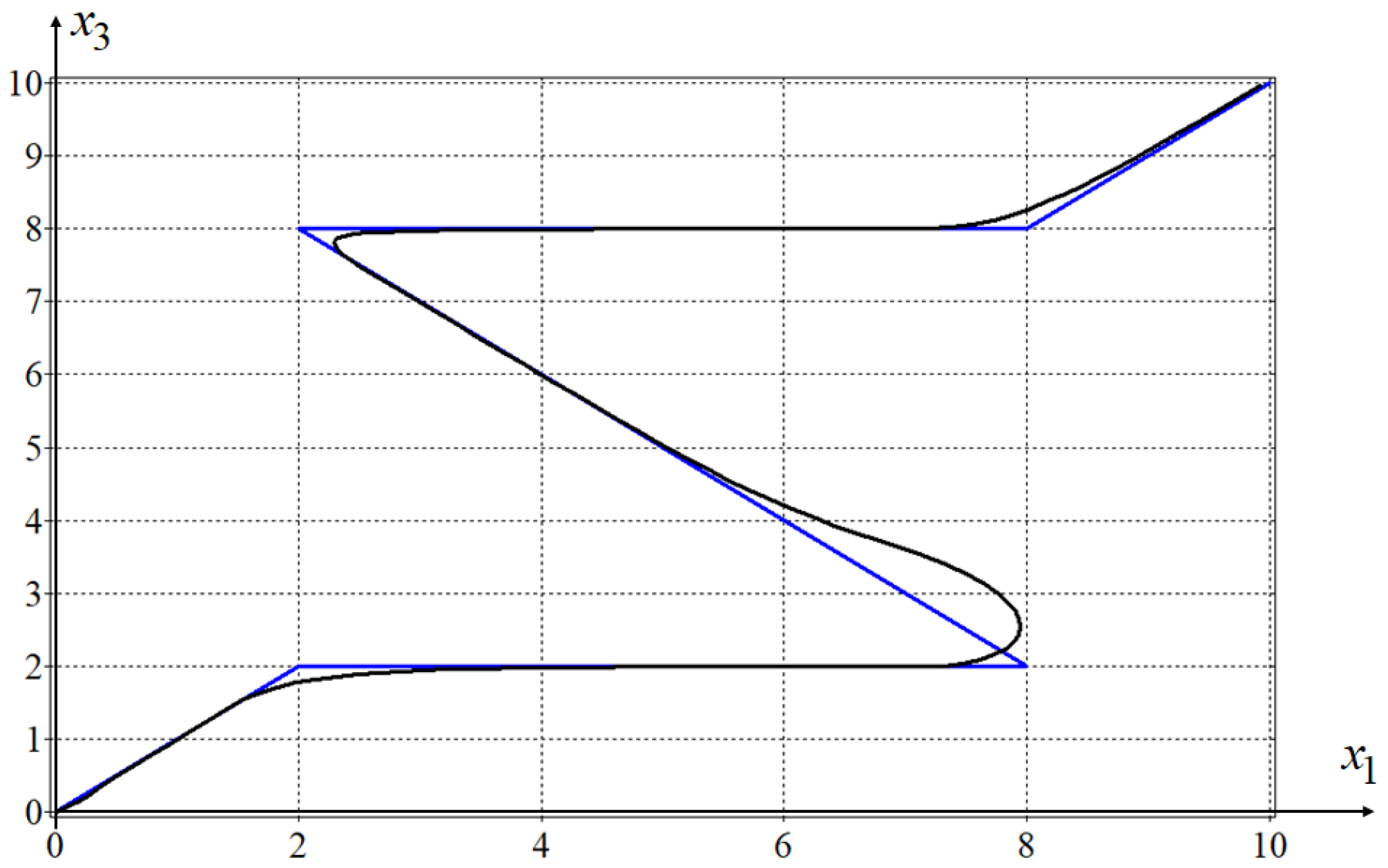
The projections of optimal trajectory (black line) and the given trajectory (blue line) on the horizontal and vertical planes are shown in Figure 3 and Figure 4.

To check the feasibility property of the obtained solution of the optimal control problem, a simulation of the control system from eight different initial states was performed: ${\mathbf{x}}^{0,1}={[-0.54.5-0.5000]}^T$, ${\mathbf{x}}^{0,2}={[-0.54.50.5000]}^T$, ${\mathbf{x}}^{0,3}={[-0.55.5-0.5000]}^T$, ${\mathbf{x}}^{0,4}={[-0.55.50.5000]}^T$, ${\mathbf{x}}^{0,5}={[0.54.5-0.5000]}^T$, ${\mathbf{x}}^{0,6}={\left[0.54.50.5000\right]}^T$, ${\mathbf{x}}^{0,7}={[0.55.5-0.5000]}^T$, ${\mathbf{x}}^{0,8}={\left[0.55.50.5000\right]}^T$.

The results of the simulation are shown in Figure 5 and Figure 6.

The results of the simulation show that the synthesised stabilisation system of the control object motion along the given spatial trajectory is not sensitive to disturbances; therefore it is realisable in a real object.

5. Discussion

The main difference of the method considered in this paper is that the trajectory stabilisation system is built entirely on the basis of machine learning by symbolic regression. Typically, a person analyses the mathematical model of the control object, identifies the control channels and determines which channels influence a particular movement of the object. Controllers are then installed in these channels and only then the parameters of the controllers are adjusted. This process is manual. A feature of machine learning control by symbolic regression is that the program is only provided with a model of the control object with a control function in the right part. The machine performs all other stages independently, without human intervention. It finds the control function in a coded form. The authors could not find a similar machine approach for the problem in other publications. Comparing the machine-learning-based approach discussed in the paper with control systems manually developed by specialists is not entirely correct, although it can be noted that the machine built a control system of equal quality. The disadvantage of the resulting control system is the complexity of the resulting mathematical expression, because the machine does not sense the complexity of calculations. We still insist that a machine search for solutions is more promising for building complex control systems than the manual approach.

In comparison to previous papers by the authors [9], in the present work, the complexity of the optimal control problem is that the given trajectory is defined in space and not in time. Instead of determining points on a given trajectory to calculate the deviation of an object from that trajectory as in prior approaches, a reference model is constructed that determines the reference motion along the trajectory. To solve the control synthesis problem, a machine learning control by symbolic regression is applied. The main goal of machine learning is to create a program to automatically write a control function. In our opinion, this approach will allow artificial intelligence to be created. Computational experiments have shown that the resulting control system has a feasibility property.

However, the proposed numerical method as all numerical methods has certain drawbacks. To obtain a solution it uses numerical techniques that include discretisation of the problem domain and approximation of the solution through an iterative computational process. Errors are accumulated and affect the final solution which is not exact, but it is still the only way to solve complex problems, such as the one presented in this paper.

Furthermore, the limitation of the proposed approach, namely, the usage of a reference model for trajectory generation, is that the velocity can be easily obtained for straight segments but might become a tricky task for differentiable trajectories.

6. Future Work

Future research is aimed at applying the presented approach to trajectories of different types. The applicability of this approach to differentiable trajectories, where the trajectory does not consist of straight segments, should be investigated. It is also necessary to investigate how the accuracy of the approximation of a smooth trajectory by straight segments affects the accuracy of the movement of the object along the trajectory, when the control synthesis problem has been solved for a reference model of movement on straight segments.