1. Introduction
Having an efficient transportation system is a necessary trait of any modern city; for this reason, great efforts are made in order to manage traffic and minimise the impact of traffic jams [
1]. Then, it follows that the ability to predict traffic in situ and in real time is crucial for a wide variety of reasons, ranging from economics to sustainability. In this scenario, the development of flexible, adaptive, and robust models can represent a great advantage to administrations and users alike. Consequently, since the early research carried out in the 1930s and 1950s, the field of traffic dynamics has received significant input from both physicist and mathematicians [
2,
3], the reason being that traffic flow can be modelled as if it were a continuous fluid.
Early traffic models assumed a linear relation between the two fundamental variables that describe vehicles dynamics, namely, the traffic density at a point in space and time (
henceforth) and the mean velocity at said point (
henceforth) [
4]. The actual relation is based on a vehicle conservation law, which is formulated as
where
denotes the flow of vehicles and corresponds to
, where
is some non-increasing function of the vehicle density, which is usually referred to as the fundamental diagram of the model [
5,
6]. Linear models of this type, however, do not capture well the complex dynamics of traffic, as the steady states to which they lead are one-dimensional [
7]. Thus, a whole set of non-linear models have been developed throughout the years to account for the anisotropies that can develop in traffic flow [
8,
9,
10,
11], in a process much like having different diffusion terms in the classical Navier–Stokes equations [
12,
13].
Among the new types of high-precision models, we find those that modify the fundamental diagram in such a way that the dependence of vehicle speed is no longer a unique function of vehicle density. Rather, it becomes another differential equation whose solution is, at the same time, part of and dependent on the model considered, thus compounding a set of non-linear models with which anisotropies in traffic due to, e.g., congestion, changes in the topology of the road considered, weather variability, or relaxation of the system, can be simulated [
14,
15,
16,
17,
18]. These models usually result in complicated coupled second-order non-linear partial differential equations of the hyperbolic kind [
19,
20,
21], which can be quite involved to interpret and whose solutions must normally be obtained with cumbersome numerical analysis that impedes their real-time usage [
22]. Here, we take advantage of the nondimensionalisation technique to solve and interpret a general non-linear second-order partial differential equation model of traffic that includes the possibility of congestion, changes in the number of vehicles due to entries and/or exits, and the relaxation of the system, offering an alternative approach to understanding traffic models.
The nondimensionalisation technique requires normalising all variables in the problem, reducing them to dimensionless independent and dependent variables and, consequently, resulting in dimensionless equations and monomials, which are the ratios between the different coefficients appearing in the problem. These monomials provide valuable information about the relative weight that each of the variables contributes to the problem and permit analysing the influence that each of the variables exerts on the others. With this information, it is possible to group the different variables by applying the -theorem, ensuring that each unknown variable appears only once within a group. Then, it is a simple task to obtain universal solutions for each of the variables, with which the original problem can be solved without having to resort to complicated numerical techniques.
The procedure for the nondimensionalisation of differential equations is well known and thoroughly explained in the literature [
23,
24]. Moreover, it has been successfully applied to a wide range of non-linear problems, such as diffusion of chlorides in reinforced concrete structures or soil consolidation [
25,
26,
27,
28], where the universal curves obtained offer invaluable information about the problems considered while offering a significant reduction in computational time with a minimal increase in error. In this article, we tackle the problem of understanding the involved behaviour of traffic by searching for the universal curves in a complex traffic model. We do so by using nondimensionalisation in the general traffic model. We show how the nondimensionalised model can be used to obtain general solutions for the behaviour of traffic in an inexpensive computational time and use it to demonstrate extreme sensitivity to initial conditions and parameter changes, which is a typical signature of deterministic chaos that explains certain odd traffic behaviours [
29]. The approach that we demonstrate here opens up new possibilities to explore complex traffic models and paves the way for real-time studies and on-site applications [
30].
The article is organised as follows: We first present the mathematical model of traffic, and describe its main characteristics. Then, we proceed with the nondimensionalisation of the model and the monomials that it leads to. Next, we show how for certain parameters, these monomials become insensitive, which means that the universal curves tend to infinity and cannot offer a proper solution due to the extreme sensitivity to the values of the parameters. Finally, we demonstrate, for the rest of the monomials, the universal solutions and their validation and draw some conclusions.
2. Mathematical Model
We consider a traffic model that allows for inbound or outbound vehicles by breaking the homogeneity of the continuity equation, such that for us, the number of vehicles is not conserved. The system of equations that models the traffic flow is, then [
31],
where
f is the relative change in the number of vehicles, a term that can be used to simulate an inflow of traffic, accounting for possible lane changes, sudden speed variations, or worsening traffic conditions.
v here is the vehicle speed, and
x is the distance. Thus, Equation (
2) accounts for the density of vehicles (
), which is spatially dependent as well as time-dependent, containing, as a consequence, the possibility of local density variations, i.e., traffic jams. Additionally, we consider the relative velocity of the congestion propagation, analogous to the sound speed of waves in a fluid medium, to be of the form
which includes parameter
to account for the possible relaxation of the resultant wave characterising traffic dynamics and which describes, e.g., alleviating measures introduced at a given time to reduce heavy traffic. Thus,
permits traffic dissipation in the model to occur. Our task is to solve this model by extracting the principal monomials using the method of nondimensionalisation [
23,
32].
First, we choose the dependent variables that will be related to one another through the independent variable; then, we define the dimensionless variables that span the monomials. To do so, we first bound density and speed, such that for a given road,
with a certain fixed maximum speed (
), and
. While
depends on the kind of road considered, typically,
, the maximum density of vehicles allowed on a given road, is fixed. The literature usually considers numbers in the range
[
33], which assume a typical average length of
metres per vehicle, plus a minimum of 1 metre in front and 1 in the back of each vehicle at any given time, and the possibility of a few longer vehicles, such as trucks. Then, the dimensionless variables are
where
and
are the initial vehicle density and speed, respectively;
is the maximum road distance considered; and
is the critical time at which the speed of vehicles goes to zero, i.e., the extreme value for the traffic jam formation time. In these expressions, we can see that
is the change in traffic density with respect to its value of maximum variation,
, which also ensures that this variable is contained in the interval
. The great advantage of introducing this new variable is that in addition to the subsequent dimensionless treatment and the obtaining of dimensionless monomials, when its value is close to 0, it tells us that traffic flows easily and, when it is close to 1, that traffic tends to get stuck. In the case of
, the dimensionless speed, the meaning is the variation in the speed of vehicles with respect to the initial speed and also relative to its maximum variation value, this variable being defined between a negative value and 1. In this case, the more negative the value is, the more often traffic jams will occur, and the closer it is to 1, the more easily traffic will flow. Finally, for both
and
, we also obtain dimensionless variables by dividing them by
and
, respectively.
We can use the variables defined in Equation (
4) to find the dimensionless form of the traffic model in Equation (
2). By also using the velocity of congestion propagation, Equation (
3), we obtain
In cases where the problem exhibits linearity or pseudo-linearity, we can assume that each term has an order of magnitude around 1 [
32,
34,
35]. Then, the factors can be extracted from the equations to obtain the relevant coefficients of the model, which are
and
respectively. Dimensionless groups are then derived from the ratios of coefficients, with the maximum number of groups being equal to the number of addends in the dimensionless equation minus one. In systems of coupled equations, certain groups may be shared across multiple equations. These groups can be further manipulated with basic mathematical operations to be presented in the most advantageous form. For instance, one optimization strategy involves ensuring that each unknown is associated with only one group [
36]. We now combine these coefficients to obtain dimensionless monomials
for each of the
equations in our traffic model:
By combining the monomials appropriately and eliminating those which appear repeated or are simply linear combinations of the others, we find the final four monomials that completely characterise Equation (
2):
We can now apply the
-theorem, which states that we can express the monomial containing the unknown as a function of all the other monomials that do not contain unknowns, such that, e.g.,
, from which the characteristic time of the problem can be obtained as
where
is some unknown function of the coefficients, which we will determine in the ensuing sections for each particular case.
3. Results
We now apply the expressions derived above to obtain specific functional forms for Equation (
11), considering certain initial conditions and particular road circumstances. Our focus here is to understand traffic jam formation as a function of vehicle speed, density, and change over time. To achieve this, we simulate the traffic model described by Equation (
2) using the Network Simulation Method [
34,
37], searching for the time (
) at which the speed goes to zero. As our starting point, we consider a given stretch of road in which, initially, conditions are those of fluid traffic, such that vehicles circulate at an initial speed (
) which is the maximum speed permitted in said road.
The Network Simulation Method is a mathematical modelling approach employed for simulating and analysing complex systems [
34,
37], particularly those characterised by multiple variables and non-linear relationships. This method revolves around the creation of an electrical network comprising interconnected nodes that serves as a symbolic representation of the physical medium or system under consideration. Within this network, the variables of interest are defined, along with their interrelationships, enabling a comprehensive exploration of the system’s behaviour and dynamics. The Network Simulation Method has been used in a wide variety of applications, including the simulation of economic [
38,
39,
40], social [
41], and biological systems [
42], among others [
43,
44,
45,
46,
47].
To comprehend the distinct effects of each variable on traffic jam formation, we fix two of the monomials at constant values throughout the time evolution of the problem. This involves selecting appropriate values for the specific variables in these monomials. Subsequently, we vary the other two monomials along a given dimension (variable) to study their influence on traffic jam formation. Since the monomials in Equation (
10) fully characterise the differential equations of the traffic model, this approach allows us to understand the individual contributions of different variables.
In the following analysis, we first explore the relationship between distance
and traffic jam formation time by keeping the speed constant, representing
vs.
. Subsequently, we examine the influence of both speed and relaxation time
on traffic jam formation time by keeping
constant, representing
vs.
. In all cases, we choose
and
, resulting in
[see Equation (
12)] for the remainder of the article.
3.1. vs. : Sensitivity to Initial Conditions
We begin by fixing
and investigating the relationship between the traffic jam formation time and distance with
. To conduct this analysis, we maintain a constant maximum density of
(vehicles/km); an initial density of
; an inflow of vehicles of
(vehicles/m·s)—meaning a new vehicle enters the road per km and per second; and a relaxation time of
(m
2/vehicles·s). Further, we select a fixed initial and maximum speed,
km/h.
Figure 1 illustrates the results of simulating the traffic model using Equation (
2) with the Network Simulation Method. The simulation is conducted for various values of distance
, determining traffic jam time
when the speed reaches zero. We calculate
with all other monomials held constant as per definition. Additionally, we present the best functional fit that provides the specific
, achieving an
close to unity in all cases.
There are two noteworthy observations about the behaviour of all
calculated in
Figure 1, providing valuable insights into relevant traffic dynamics. The first is that as the distance approaches zero, the traffic jam formation time diverges to infinity. This outcome is expected; if the stretch of road considered is sufficiently small, any vehicle present can be considered a traffic jam. This implies that the model is only valid for distances spanning several vehicle lengths, as defined by the maximum allowed density of vehicles,
. This density depends on the specific speed considered, changing from ∼50 in
Figure 1a,b, featuring initial and maximal speeds of 20 km/h and 50 km/h, respectively, to ∼20 in
Figure 1c, where the speed considered is 100 km/h.
On the opposite end, we observe that the traffic jam formation time is essentially constant, indicating that given certain speed and density of vehicles, traffic jam formation is inevitable. This also suggests that higher speeds lead to slower traffic jam formation, but the latter can also occur in shorter distances.
The asymptotic behaviour with constant independent of and distance and the smallness of the fitting parameters that control the influence of on indicate extreme sensitivity to the values of the variables in the problem. Minute differences can result in significant changes in the predicted traffic jam time. Neither the exact equations and their numerical solution nor the fitted models can capture such behaviour, leading to substantial differences in the predicted traffic jam time for apparently similar initial conditions.
This sensitivity explains a phenomenon experienced by any driver on the road—the apparent spurious formation of traffic jams following smooth conditions in what seemed to be dense but fluid traffic [
48,
49,
50]. It also suggests that traffic jam alleviation measures should focus on reducing the number of incoming vehicles on the road (namely,
f) and accelerating relaxation times. Any other measure is likely to have a random or negligible impact.
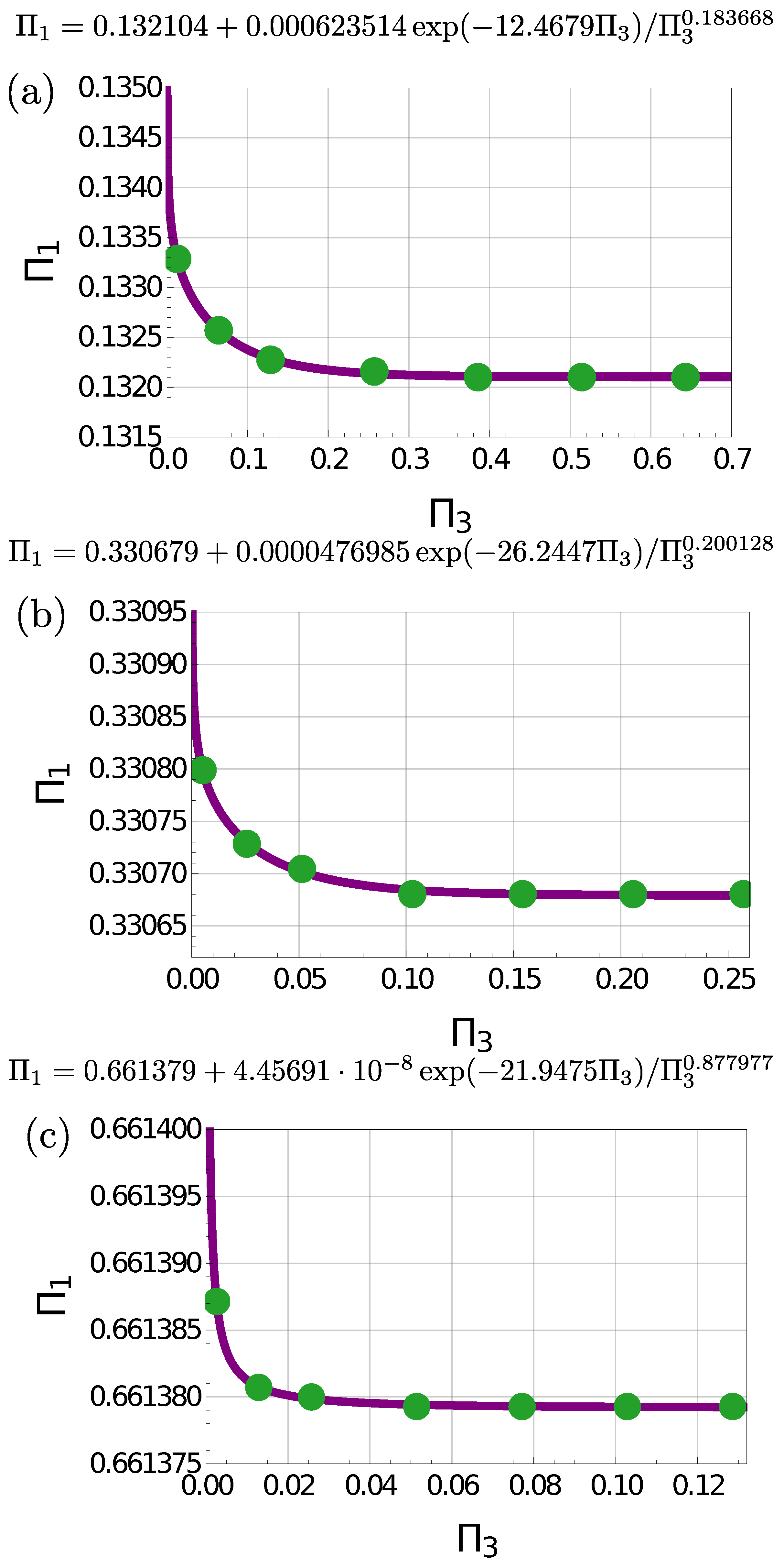
3.2. vs. : Speed Dependence
We now examine the relationship between and while keeping constant (with throughout, as done previously). We seek to understand the impact of speed and relaxation measures on traffic jam formation and to illustrate how the nondimensionalisation of the differential equation system facilitates the accurate, simple, and efficient modelling of traffic dynamics.
Initially, we determine the traffic jam formation time (
) by solving the exact model for two instances of the relaxation parameter (
) while varying the speed (
) and keeping the ratio
constant to maintain
unchanged. By selecting
and
, we obtain the results depicted in
Figure 2a (with
) and b (with
). In both cases, we fit the data points to a functional form
, as shown above each figure with the best-fitting parameters. This functional form effectively reproduces the traffic behaviour with a near-unity
. Subsequently, we use these fits to validate the model.
Observing the results in
Figure 2, we note that the traffic jam formation time is highly dependent on speed, favouring fast traffic jam formation at slower speeds. This is due to the fact that for slow-moving vehicles, the addition of more traffic through the
f term increases the density faster than it can dissipate it. This suggests that alleviating measures, once the speed is limited to a certain high value, should focus on introducing relaxation mechanisms, such as facilitating road exits. This is demonstrated in
Figure 3, where instead of changing
through speed, we fix
at three different values and change
using the Network Simulation Method. We observe a greater sensitivity to the relaxation parameter, indicating that a small relaxation parameter can significantly extend the traffic jam formation time.
Finally, note that all panels in
Figure 2 and
Figure 3 present similar results with different ranges of validity. This suggests the general applicability of the traffic model we are analysing and demonstrates that the nondimensionalisation technique accurately captures the correct dynamics over a wide range of parameter regions. This means that it can be effectively used to simplify the resolution of traffic differential equations, reducing the required time and enhancing their applicability under real-time conditions. To demonstrate the predictive capabilities of the obtained functionals,
, we validate the model using the data from
Figure 2b and interpolate for different cases.
Model Validation
We now validate the methodology employed and the results obtained for the functionals
by choosing various study cases, displayed with their corresponding parameters of choice in
Table 1. For these, we calculate both
and
, which shows that there is a slight remaining dependence on
, which is nonetheless inconsequential for the results.
All the models presented in
Table 1 were deliberately selected to encompass a broad spectrum of parameters. This intentional diversity aims to underscore the comprehensive applicability of the nondimensionalisation methodology and the universality of the results. The chosen models span a wide range of speeds, allowing us to calculate traffic jam times at various distances. Simultaneously, we explore changes in the relaxation parameter and an increase in the number of allowed incoming vehicles. Intriguingly, despite the expected delay in traffic jam formation due to speed increase, we observe a counterintuitive trend: the traffic jam formation time decreases across the studied cases. This is due to the role played by the term inflow of vehicles,
f, which highlights its importance as the key factor requiring attention for preventing traffic jam formation, advocating for targeted interventions on this parameter to mitigate traffic congestion.
It is worth noting that in all cases, we set the maximum allowed density (
) to the highest conceivable value [
33], essentially testing the model’s validity at the extremes. This approach ensures the robustness of the model across a range of scenarios, validating its efficacy even under conditions where traffic jam formation might be delayed due to lower density limits.
With the value of
, one either chooses to calculate
using one of the following equations:
or, provided that the values of
and
do not coincide with those chosen in
Figure 2b, interpolates between them to obtain
, from which we can readily obtain the traffic jam formation time,
. We compare this with the exact result
for those same parameters obtained by solving the exact model with the Network Simulation Method [
34,
37]. An extraordinarily good agreement between exact result and model is found.
Figure 4 displays the results for the speed evolution obtained by solving the exact traffic model differential equations numerically, up to the point at which traffic jam formation occurs, signalled by the speed reaching zero.
4. Discussion
In this article, we introduce a generalised traffic model that incorporates discontinuities and anisotropies through a relaxation parameter, along with the ability to dynamically adjust the number of vehicles over time. Using a numerical approach, we determine the traffic jam formation time as the time at which the speed of vehicles drops to zero. This is a necessary approximation taken in order to have a definite rule that can be used for any parameter set. Note that actually, traffic jam formation starts earlier, as the density of vehicles overcomes a critical value. However, said critical value is dependent on the choice of parameters f and and the initial conditions and thus cannot be used as a universal measure to validate the model, hence our choice. We understand that this represents an advantage, as it allows us to demonstrate our approach and perform a universal analysis, but it is also a drawback, as it somewhat limits the accuracy of the prediction. Nonetheless, a precise traffic jam formation time prediction can be obtained by simply shifting the definition for a particular set of parameters; it is, therefore, not a limitation of our approach. Future work will explore the different particulars of the traffic model that we generally present here, as the traffic jam formation time offers a unique benchmark, crucial to evaluating the model’s ability to reflect real-world road conditions.
By using nondimensionalisation, we decompose the traffic differential equations into their principal monomials, establishing unique relationships among dimensionless variables. This technique enables a more efficient determination of the traffic jam formation time, or any other parameter, compared with solving the entire model numerically, without a noticeable loss of precision, and shows the stability regions of the model by easily demonstrating where divergences appear. The insights that we gain in this way can, therefore, be used to determine efficient ways to manage traffic and show that the focus should be placed not on long-term prediction but rather on rapid adaptable measures.
Our initial study reveals a high sensitivity of the model to certain parameters, a characteristic feature of deterministic chaos. This sensitivity explains the seemingly irrational occurrence of traffic jams under fluid driving conditions. Such instabilities, common in complex models with coupled partial differential equations, result in significant variations over time due to slight changes in certain parameters. This leads to exponential numerical complexity, making long-term predictions challenging, as the system effectively behaves in a random manner after a critical time. This behaviour is evident in the divergence to infinity or constant values of the functionals of the monomials. Such behaviour is critical, as it inherently limits our ability to predict traffic beyond a certain point, regardless of the complexity of the modelling that we use, and means that traffic prediction models should rather focus on short-term prediction and traffic-alleviating measures in real time, a goal for which our analysis is specially suited, given the speed boost provided by simplifying the model while maintaining accuracy through nondimensionalisation.
Expanding our study, we analyse different relationships between the monomials and validate the results by comparing them to exact simulations. The analysis demonstrates a remarkable ability to predict the traffic jam formation time based on the obtained functionals, eliminating the need for complex simulations each time. This simplification reduces the prediction problem to interpolating the correct functional. While the nondimensionalisation technique is limited to a specific range of values, its solutions are universal enough to be applied to a broad range of traffic situations, offering a simple and straightforward method to obtain key parameters. It is true and a limitation of our and any traffic modelling approach that not all variables affecting real-life traffic can be taken into account, but it is also true that by introducing a traffic inflow and relaxation parameters, we provide our model with enough flexibility to accommodate a wide range of nuances, such as weather conditions or certain human behaviours, which can be thoroughly explored with the technique presented here.
5. Conclusions
Having reliable traffic models that can be utilised in real time is a crucial asset for any society. However, traffic models often prove to be cumbersome, complex, and difficult to solve, limiting their interpretability and applicability. In this article, we consider one such complex model and demonstrate that it is possible to simplify its analysis without compromising the accuracy of the short-term predictions that can be drawn. We do so by nondimensionalising the model and thoroughly analysing the resulting monomials, with which we obtain universal solutions. Focusing on traffic jam formation as a benchmark, we show extreme sensitivity to initial conditions and parameter changes and demonstrate the validity of our approach, which shows that the simplified model obtained through nondimensionalisation has essentially the same accuracy as the solutions of the full-model equations.
Nondimensionalisation techniques can become an essential tool for simplifying complex traffic models in transportation engineering. By normalizing variables and removing physical units, the mathematical expressions are greatly simplified for analysis. This approach is particularly useful in traffic simulations, where various interacting factors contribute to model complexity. Identifying dimensionless parameters streamlines the system’s representation. Simultaneously, integrating network simulations is crucial to solving these models. These simulations allow for a detailed exploration of traffic dynamics and intervention impacts, offering valuable insights for optimizing urban mobility and transportation systems through informed decision making.
Following the first demonstration of the usefulness of nondimensionalisation for traffic models, future dedicated work will explore in detail the onset of chaotic behaviour and the extreme dependence of minor variations on input parameters, which have a huge impact on the ability to make long-term predictions, which suggests that these models should target quick response to changing traffic conditions rather than extending the predictions in time. Furthermore, given the simplicity that nondimensionalising the model brings, we will analyse the parameter range in full detail and include different parameters that account for various traffic effects. Additionally, future work will also test the validity of the model beyond the mere numerical analysis by using real traffic data.

 ,
, 


