Article

Analysis of Higher-Order Bézier Curves for Approximation of the Static Magnetic Properties of NO Electrical Steels

Institute of Electrical Power Engineering, UM FERI, Koroška cesta 46, 2000 Maribor, Slovenia
*
Author to whom correspondence should be addressed.
Mathematics 2024, 12(3), 445; https://doi.org/10.3390/math12030445
Submission received: 18 December 2023 / Revised: 24 January 2024 / Accepted: 27 January 2024 / Published: 30 January 2024

Abstract

:
Adequate mathematical description of magnetization curves is indispensable in engineering. The accuracy of the description has a significant impact on the design of electric machines and devices. The aim of this paper was to analyze the capability of Bézier curves systematically, to describe the nonlinear static magnetic properties of non-oriented electrical steels, and to compare this approach versus the established mathematical descriptions. First, analytic functions versus measurements were analyzed. The Bézier curves were then compared systematically with the most adequate analytic functions. Next, the most suitable orders of Bézier curves were determined for the approximation of nonlinear magnetic properties, where the influence of the range of the input measurement dataset on the approximation process was analyzed. Last, the extrapolation capabilities of the Bézier curves and analytic functions were evaluated. The general conclusion is that Bézier curves have adequate flexibility and significant potential for the approximation and extrapolation of nonlinear properties of non-oriented electrical steels.

1. Introduction

The magnetic properties of soft magnetic materials are highly nonlinear and reflect intricate underlying phenomena in hysteresis behavior. In engineering applications, these properties are often described using basic magnetization curves, e.g., the anhysteretic curve, the first magnetization curve, the major loop, and the minor loops. For example, the major loop represents the input data of several well-known hysteresis models [1,2,3]. Examples of using the anhysteretic curve as input data are the widespread Jiles–Atherton hysteresis model and its variations [4,5] and various finite element simulation tools. Hysteresis models are used to describe nonlinear magnetization and power loss in iron cores, whereas the nonlinear behavior is indispensable in the design of electromagnetic machines and devices [6,7]. For these reasons, it is important to find adequate methods or analytic functions to describe such nonlinear curves with high accuracy and with low computational power.
Researchers have applied various approaches to model all the discussed magnetization curves. On the one hand, researchers try to establish adequate links between the physical parameters of materials and various mathematical descriptions, which would result in adequate physics-based material models [4]. This is a very complex task, and essential for understanding the intricate phenomena within soft magnetic materials, and, consequently, for their design and optimization processes. The complexity arises from the fact that hysteresis is a macroscopic property that emerges from the collective behavior of microscopic entities, and this behavior can be influenced by a multitude of factors [8]. On the other hand, researchers also try to model nonlinear magnetization in a more practical way to predict the magnetization behavior, which is based on measured datasets. These models are phenomenological, i.e., they simply attempt to describe nonlinear relationships with the assumption that the modeled relationships extend past the measured values without a deep understanding of the underlying mechanisms [9,10,11,12]. These models are equally as important as the physical ones, and are essential in applied engineering, where the existing soft magnetic materials are applied in electromagnetic devices and machines. The most important requirements are accuracy and computational simplicity. A common and straightforward method is to use mathematical functions [2,10,13] or curves [14] that approximate the data obtained from measurements. This method has its difficulties, as it needs costly and specific instruments for measurement, and the data obtained may be limited in both amount (i.e., volume) and quality. To measure the magnetization curves, the measurement equipment can reach different levels of saturation, depending on its capability. The equipment also has different degrees of accuracy that affect the noise and errors in the obtained curves. The quality of the approximations depends on several factors: the size and noise level of the input dataset, the properties of the functions used, and the type of the fitting method. For example, an analysis based on the application of sigmoid functions is described in [15]. The authors investigated the relevant sigmoid functions and used them to construct the major hysteresis loop. Recently, the sigmoid functions from [15] were modified and fitted using different optimization algorithms to match measured data [10]. The modified analytic functions offered more degrees of freedom during the fitting process. In this paper, we examined different methods for estimating and extending the data obtained from measurements.
An approach used in many fields for the description of a wide range of different shapes and curves is (classical) Bézier curves. Bézier curves enable the construction of free-form curves and surfaces. The shape of a Bézier curve depends on the placement of the so-called control points. This feature makes them intuitive, easy to implement, and flexible. It is possible to construct very complex shapes only by placing control points in adequate positions. Bézier curves were first used for the shape optimization of automobile bodies [16]. Nowadays, these curves are used widely in computer graphics and animation. Examples of using them in computer graphics are font generation (Chinese [16] and Arabic [17]), image processing, and path design in various animations. However, they are not limited to the field of computer graphics. Due to their simplicity and continuous curvature, Bézier curves are being used in path planning for ground vehicles [18,19,20] and for unmanned aerial vehicles [21]. Their free-form ability made them popular in the field of shape design. An example of shape optimization with Bézier curves is the modeling of laminated plates of variable stiffness [22]. To expand their usability in shape optimization, Bézier curves are used to construct circular arcs in CAD applications (e.g., SolidWorks) [23] using mainly cubic Bézier curves [22]. The free-form ability to represent various shapes and geometries enhanced and is useful in the field of additive manufacturing, e.g., for the topology optimization of electrical machines [24,25]. Their ability to fit any dataset smoothly also makes them useful in the field of electrical engineering. The applications include the modeling of the flux linkage characteristics of a switched reluctance motor [26] and the modeling of PV module characteristics [27,28].
Classical Bézier curves are often used for simple smooth curve approximations. The number of control points defines the order of the corresponding Bézier curve. The order can be set to any arbitrary number for more flexibility, but it will increase the complexity due to an increasing number of control points [22]. Furthermore, Bézier curves constructed by a large number of control points are numerically unstable [19], and the calculation is slower since additional coordinates have to be calculated. For this reason, an alternative approach is to join low-order Bézier curves together in a smooth way to form a composite curve. This concept is called piecewise Bézier curves, and it builds a curve as a union of Bézier curves connected end to end [29]. Using this concept, even more complex shapes can be described by joining a larger number of lower orders of Bézier curves. A few rules must be followed to obtain a smooth curve when joining Bézier curves, e.g., the so-called parametric continuity rules [22,30]. Bézier curves are also used for spline interpolations, especially in the known B-spline group. Any piecewise Bézier curves with arbitrary order can be converted into a B-spline, and any B-spline can be converted into one or more Bezier curves [29]. The B-spline curve has one main disadvantage compared with piecewise Bézier curves. The B-spline concept requires more computation, and the mathematics used to describe them are more complicated [29].
Based on the discussed flexibility that Bézier curves offer, especially the smooth fitting of datasets, we performed an analysis of the Bézier curve fitting process on various fundamental magnetization curves of non-oriented (NO) electrical steels (i.e., the anhysteretic curve, the major loop, and the first magnetization curve). This work is an extension of the preliminary study [31], and the aim was to investigate the approximation capabilities of classical Bézier curves systematically. We limited this study to classical Bézier curves because of their straightforward approximation of datasets without the need to implement additional rules, e.g., the continuity rules [22,30]. To demonstrate their ability to approximate magnetization curves, we identified established analytic functions [10,15] in parallel and performed a systematic comparison based on the deviation from the measured curves. We analyzed the deviation from the measured data in different regions of individual curves, e.g., the high-permeability region and the region of high saturation. This analysis resulted in the identification of the most suitable orders of classical Bézier curves and the most adequate analytic functions for different input datasets. The high-saturation region is, in most cases, very challenging to evaluate experimentally; therefore, we further analyzed the extrapolation capabilities of the identified Bézier curves and analytic functions. The main challenge during the curve-fitting process was to find the position of the control points, which determine the shape and curvature of the curve [18]. The main goal was to find a precise and elegant way to represent the observed data mathematically beyond the range of observation and to examine how the size of the input data sets affected the results.
The article is split into six sections. Section 2 presents the considered analytic functions, as well as the description of the theoretical background and properties of the Bézier curves. Two methods are presented for calculating the Bézier curves. The materials and the methodology used are presented in Section 3. Section 4 contains the obtained results. The influence of the order of Bézier curves on the approximation of the measured data is analyzed. Additionally, the extrapolation capabilities of Bézier curves of selected orders and analytic functions are analyzed. In Section 5, a discussion is provided. Finally, in Section 6, the concluding remarks are presented with a description of future work.

2. Mathematical Descriptions of Nonlinear Magnetic Properties

Mathematical functions, which are adequate for the description of the nonlinear curves in hysteresis, must have specific properties. They must be continuous, differentiable, single valued, and monotone; have odd symmetry; approach saturation polarization J s , as magnetic field strength H tends toward negative or positive infinity (e.g., in ideal cases they have asymptotes); and must have a knee point where the second derivative reaches its minimal value [4].
Natural candidates that have those properties are the so-called sigmoid functions. The aim of this work is to introduce and analyze a novel concept for the approximation of nonlinear magnetic properties that is based on curves instead of functions, where classical Bézier curves of different orders are considered.

2.1. Analytic Functions

Analytic functions that describe a curve shaped in the form of the letter “S” are called sigmoid functions. Besides their shape, sigmoid functions have further important properties. Sigmoid functions are real valued, differentiable, and have a pair of horizontal asymptotes [15]. Due to their intrinsic properties, sigmoid functions are suitable candidates to describe nonlinear magnetic properties. The described favorable basic properties are the reason for the frequent use of sigmoid functions in the description of the discussed magnetization curves [4]. The most adequate (and, for the discussed purpose, applied) sigmoid functions [10,15] are presented in Table 1 with Functions (1)–(5). In addition, many functions exist that have a similar shape to sigmoid functions but do not have all their properties, e.g., do not have horizontal asymptotes. Such functions are still applicable to the discussed problem and are widely used in applied engineering. During the preliminary analysis [31], we determined that the inverse hyperbolic sine function is promising, especially in the saturation region, because of its logarithmic character for higher input values. Therefore, the inverse hyperbolic sine of Function (6) was included in the presented analysis.
Original analytic functions were modified with additional parameters to enable better agreement with the measured data during the approximation process. Functions (1)–(6) all have parameters:
  • a —determines the value of the asymptote;
  • b —controls the slope of the curve;
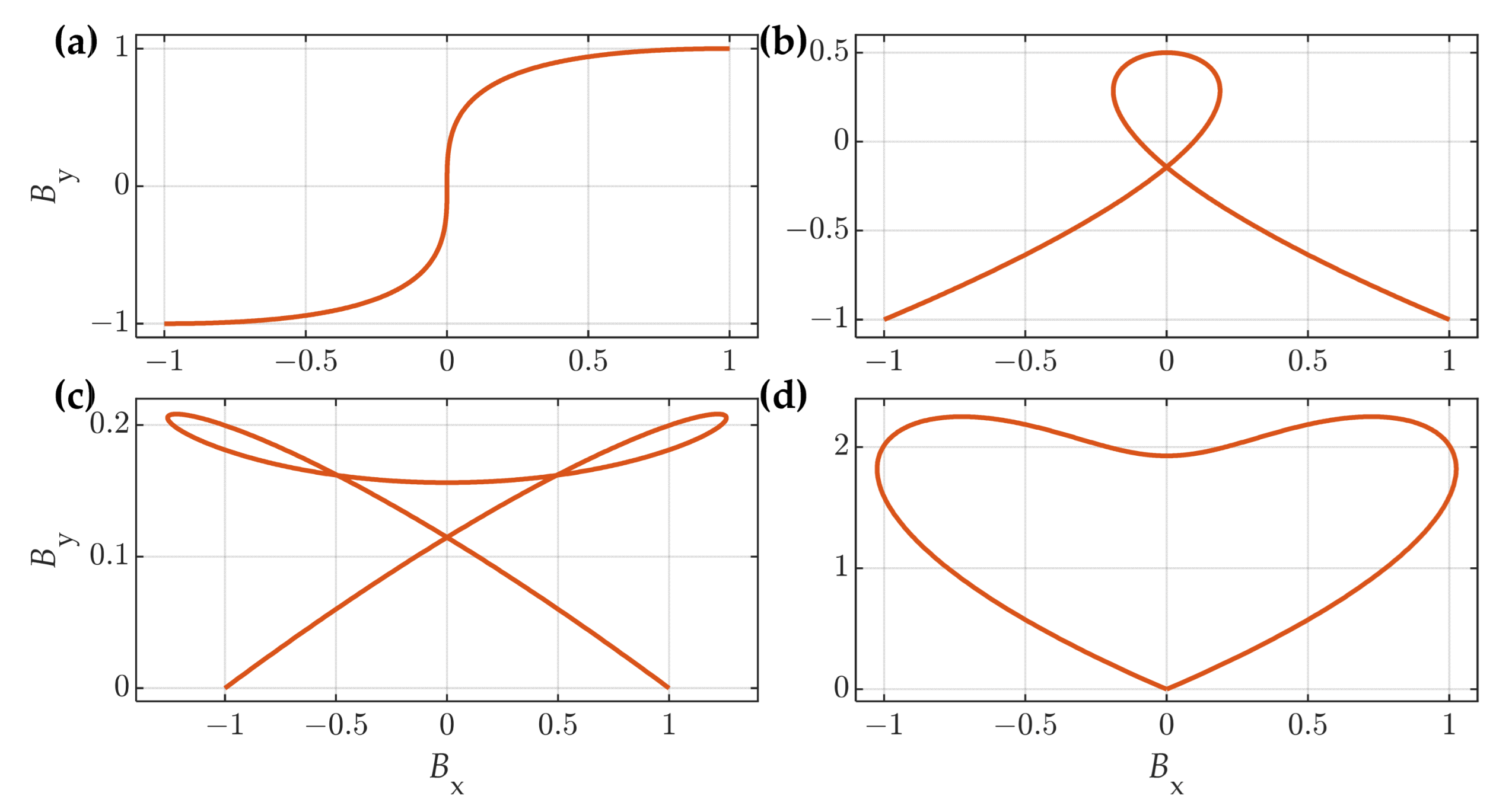
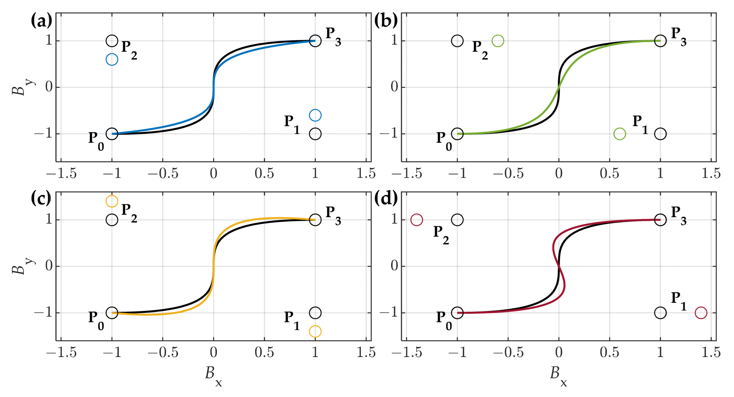
  • c —enables the shifting of the function along the x-axis in an xy-coordinate system [15].
Functions (1) and (3) have a fourth parameter d , which also influences the slope [15].
Functions (1)–(4) are analytic functions without any physical background. In contrast to this, the Langevin function (Function (5)) has a physical origin. The Langevin function is a special case of the quantum mechanical Brillouin function when the function is limited to infinity [32]. The function was originally derived for paramagnets. Because of its physical foundation, it is used in many models to describe the magnetization curves, e.g., in the Jiles–Atherton hysteresis model [5]. Further, in applied engineering, the so-called Frölich–Kennelly approximation is often used for the description of nonlinear properties, especially for extrapolation purposes [6,33]. The Frölich–Kennelly equation has an equivalent mathematical description in the Elliot function (Function (3)). Therefore, all results obtained for the Elliot function also apply for the Frölich–Kennelly description.
In addition, we analyzed the inverse hyperbolic sine function (Function (6)). Generally, the inverse hyperbolic sine function has all the properties needed for adequate approximation of nonlinear magnetic properties. The difference compared with sigmoid functions (Functions (1)–(5)) is that the inverse hyperbolic sine function does not have asymptotes. However, the function value of the inverse hyperbolic sine function increases almost linearly (with a small slope), as the input x values increase at very high values. For that reason, parameter a has a scaling role for the inverse hyperbolic sine function.
Figure 1 presents a graphical comparison of the functions from Table 1. The parameters were set to a = 1 , b = 1 , c = 0 , and d = 1 for the sigmoid functions. Such a choice ensured that Functions (1)–(5) approached horizontal asymptotes at −1 and 1, as the x-value tended to negative and positive infinities, respectively. For the sake of graphic comparison, the parameters of the inverse hyperbolic sine function were set to a = 1 / asinh 5 , b = 1 , and c = 0 to ensure that the first and last point of the function reached values of −1 and 1 in the presented interval x [ 5 ,   5 ] in Figure 1.

2.2. Bézier Curves

Bézier curves are parametric curves with Bernstein polynomials as their basis functions. Paul de Casteljau contributed significantly to their first development, but they are named after Pierre Bézier, who invented them in 1962 and made them widely popular for the shape design of automobile bodies while working for Renault [16,19]. Parametric curves are not defined as y ( x ) dependencies, but they describe the shape of a curve based on a (local) input variable t that is defined along the curve. Variable t is 0 at the start of the curve and 1 at the end. For each value of t , two values are defined (i.e., x t and y t ), which, combined, define the coordinates ( x ( t ) , y ( t ) ) of all the points on the curve. This means that the coordinates of a Bézier curve are obtained using two polynomials x t = B x t and y t = B y t [34]. Due to this property, parametric curves enable the description of highly complex curves. The free-form ability of Bézier curves, explained in Section 1, is demonstrated in Figure 2. It is possible to form a single-valued curve, as shown in Figure 2a; self-intersecting curves, as shown in Figure 2b,c; and complex shapes, as shown in Figure 2d.
Bézier curves are defined by their order n and a corresponding set of ( n + 1 ) control points P = ( P 0 , P 1 , , P n ) . Each control point has its x and y coordinates P i x i , y i ( i = 0 ,   1 , , n ) in the 2D Cartesian coordinate system. Considering order n and corresponding vector of control points P , the Bézier curve B t = B x t , B y t can be expressed in polynomial form by Equations (7) and (8)
B x t = x t = i = 0 n b i , n t x i ,     0 t 1 ,
B y t = y t = i = 0 n b i , n t y i ,     0 t 1 ,
where b i , n t represents the Bernstein basis polynomials and ( x i , y i ) are the coordinates of control point P i . The Bernstein basis polynomials of order n are defined by Equation (9) [18]:
b i , n t = n i t i 1 t n i ,     i = 0 , , n
where t 0,1 , in which 0 is the starting point of the curve and 1 is the end point of the curve [18], and n i is a binomial coefficient defined by Equation (10):
n i = n ! i ! n i !
Besides Bézier curves, Bernstein polynomials are also known as basis functions for splines [35]. The basis functions of the Bézier curve can be enhanced to be able to reproduce various shapes, such as those presented in [30]. De Casteljau’s recursive algorithm is used to evaluate Bézier curve polynomials because of its numerical stability [18].
Another feature of Bézier curves is their matrix representation, which allows for a straightforward calculation of the polynomial coefficients for functions B x t and B y t . For a Bézier curve of order n , the matrix equation is defined by Equation (11) [36]:
B x t = t n t n 1 t 1 M B é z , n x 0 x 1 x n 1 x n
The B x t polynomial of the Bézier curve is obtained with Equation (11). To obtain the B y t polynomial of the Bézier curve, the y coordinates of control points P i must be considered in Equation (11). The matrix M B é z , n is an n + 1 × n + 1 -sized coupling matrix between the variable t and the control point’s coordinates P . By evaluating the matrix M B é z , n for Bézier curves of orders of up to 6 [36,37], the general form of matrix M B é z , n for curves of order n is determined by Equation (12) [38]:
M B é z , n = n 0 n n n 1 n 1 n 1 n n 1 1 1 n n 0 0 n 0 n n 1 n 1 n 1 n 2 n n 1 1 0 0 n 0 n n 2 n 1 n 1 n 3 0 0 n 0 n 1 n 1 n 1 0 0 0 n 0 n 0 0 0 0
Each non-zero element in M B é z , n is calculated as the product of two binomial coefficients by applying Equation (10). The elements within M B é z , n have a positive or negative sign depending on the matrix order. A general rule is that the main counter diagonal elements of matrix M B é z , n always have a positive sign, and then the sign alternates between negative and positive for all other diagonals above the main counter diagonal. The formation of matrix M B é z , n is presented in [36,37].

2.2.1. Properties of Bézier Curves

The basic properties of Bézier curves are:
  • First, control point P 0 defines the beginning, and the last control point P n defines the end of the curve.
  • The tangent vector formed by the first two control points P 0 and P 1 P 0 P 1 ¯ defines the initial direction, and the tangent vector formed by the last two points P n 1 P n ¯ defines the ending direction of the curve.
  • The Bézier curve lies within the area that is formed by the control points [18,19,20].
Furthermore, an important property of Bézier curves is the straightforward calculation of its derivative in terms of the variable t . If the Bézier curve for x coordinates is x t = B x t and for y coordinates is y t = B y t , then the first derivative d y / d x is calculated by Equation (13):
d y d x = d y / d t d x / d t
and the second derivative d 2 y / d x 2 by Equation (14):
d 2 y d x 2 = d d t d y / d x d x / d t
The equations for the first and second derivatives allow for the calculation of the curvature of Bézier curves [18,19,39]. Bézier curves offer the possibility to form symmetric curves. Symmetric Bézier curves are generated by placing pairwise control points into symmetrical positions [40].

2.2.2. Impact of the Control Point’s Placement on the Bézier Curve

In this subsection, we demonstrate the impact of the positioning of control points on the shape of a cubic (i.e., order of n = 3 ) Bézier curve. As presented in Figure 2, Bézier curves enable the formation of various shapes—continuous single-valued curves, as shown in Figure 2a; self-intersecting curves, as presented in Figure 2b,c; and closed shapes, as shown in Figure 2d. Figure 3 shows the various possibilities regarding the change in shape of a cubic Bézier curve from Figure 2a only by changing the position of the control points P 1 and P 2 (the first P 0 and last P 3 control points have fixed positions).
We chose to fix the first and last points for the presented comparison to show the variety of curves that start and end in the same points. As explained in Section 2.2.1, the starting and ending directions of the curve were defined by the tangents P 0 P 1 ¯ and P 2 P 3 ¯ , respectively. The cases shown in Figure 3a,b are examples of changing the slope and curvature by moving the control points but preserving the property analogous to a single-valued function. In the case presented in Figure 3c, when the control point P 1 was below control point P 0 and P 2 was above P 3 , we obtained an overshoot over the normalized value of 1. That behavior is not adequate for the description of magnetization curves. Another nonphysical behavior was observed when the absolute values of the x coordinates of points P 1 and P 2 were higher than the x values of the last and first control points, respectively, as shown in Figure 3d. The obtained curve was not single valued in respect to x and thus not appropriate for the description of magnetization curves. Control points are decisive for the curvature and shape of the final curve [26].

3. Methodology

3.1. Assumptions and Limitations

The discussed analytical functions in Section 2.1 have limited ability to approximate various curves with high accuracy because they have only three or four adjustable parameters. In contrast to this, the Bézier curves can be based on many theoretically arbitrary control points; therefore, they offer higher flexibility for the approximation of measured data.
The focus of the presented analysis was on a systematic analysis of which functions and curves would result in the best fit based on different sets of measured data. Further, the extrapolation capabilities of the presented functions and curves were analyzed. During the analyses, we assumed that different sets of measured data for two NO steels were available. We limited the analyses to the application of the presented analytical functions and classical Bézier curves of different orders. One of the goals was to identify the most adequate orders for approximation of the discussed curves.

3.2. Measured Data

The analysis was performed systematically based on measured characteristic magnetization curves J ( H ) , where J is the magnetic polarization and H is the magnetic field strength. In the analysis, we considered three of the most basic curves that describe the nonlinear properties of soft magnetic materials:
(1)
First magnetization curves;
(2)
Anhysteretic curves;
(3)
Descending branches of the major loops.
We determined the discussed curves for two NO electrical steels with different thicknesses, i.e., 0.27 mm (NO27) and 0.35 mm (NO35), which are both commonly used in contemporary electrical machines. The measurement setup was based on a single sheet tester within a computer-aided measurement setup, in accordance with the International Standard IEC 60404-3. The measurements were performed at low excitation frequencies (i.e., under the so-called quasi-static conditions) up to H = 50   k A / m at 5000 J -equidistant measurement points. Based on the measured curves, it was assumed that H = H s = 50   k A / m was the saturation point of both materials. Consequently, the available measured dataset was H m e a s = H s , H s , where H s , H s denotes the interval of the discrete measured dataset, starting from H s and ending with H s .
The anhysteretic curve was calculated as the average value of polarization J between the ascending and descending branches of the major loop.

3.3. Definition of the Data Subsets and Evaluation (Sub)Regions

All the discussed functions and curves were evaluated systematically on different input subsets H i n of the available measured data H m e a s (i.e., H m e a s = H s , H s ). The input subset H i n was, in all cases, a subinterval of the measured data H m e a s , i.e., H i n H m e a s . The evaluation subregions H e v a l were defined within the discussed input subsets H i n . Special attention was paid to evaluation of the following characteristic subregions:
(1)
The high-permeability (HP) subregion ( H e v a l , 2 = H 1 , H 1 );
(2)
The saturation (SAT) subregion ( H e v a l , 3 = H i n , m a x , H 1 H 1 , H i n , m a x );
(3)
The extrapolation (EXT) subregion ( H e v a l , 6 = H s , H i n , m a x H i n , m a x , H s ).
The HP and SAT subregions were important for the first part of the analysis, i.e., evaluation of the approximation capabilities, whereas the EXT subregion was crucial for the analysis of the extrapolation capabilities. These subregions are very important in applied engineering and are presented schematically in Figure 4.
The input subset H i n used in the process of fitting analytical functions and Bézier curves is plotted in blue in Figure 4. The measured data between H i n , m a x , H i n , m a x represented the input subset H i n in individual cases for approximation, as presented in Figure 4a. It was slightly different for the case of extrapolation, where, additionally, the saturation points H s were added to both sides of the input subset H i n , highlighted with the blue cross in Figure 4b. The characteristic subregions of the magnetization curves were identified in both cases. Considering those subregions, the measured data were divided accordingly into evaluation subsets, denoted with H e v a l , 1 to H e v a l , 6 and presented in Figure 4a,b. This approach and division enabled us to perform a systematic analysis via local evaluation of the goodness of fit of the approximated curves in specific subregions individually as well as a global evaluation on the input subset H i n .
It is important to note that H s and H 1 were fixed at H s = 50   k A / m and H 1 = 1   k A / m , respectively. In contrast to this, H i n , m a x was varied (i.e., 1, 2, 5, 10, 15, 20, 30, 40, and 50 kA/m) and determined various input datasets for approximation and extrapolation of the discussed functions and curves.

3.4. Curve Fitting

The parameters ( a , b , c , and d ) of the analytic function from Table 1 were fitted to the input subsets H i n of the measured magnetization curves using the Matlab function fit by applying the nonlinear least squares method.
For the process (i.e., the placement of control points) of fitting Bézier curves to the input subsets H i n , we applied the differential evolution (DE) algorithm [10,41]. We set the value of the mutation factor to 0.5 and the crossover factor to 0.7 and used the DE algorithm for 15,000 iterations for each curve. In each iteration, the x and y coordinates of the control points were calculated to minimize the deviation of the calculated Bézier and measured magnetization curves. Within the process, the first and last control points (which were assumed to be equal to the first and last points, respectively, of the input subset H i n ) were fixed according to the adequate position of the measured curve. The goal was to determine the intermediate control points. To find the optimum values, we minimized the objective function F in Equation (15):
F = i = 1 N m a x J i n , i ( H i n , i ) J c a l c , i ( H i n , i ) 2 ,
where J i n , i ( H i n , i ) are the input measured values of the magnetic polarization at the corresponding magnetic field strengths H i n , i , J c a l c , i ( H i n , i ) is the magnetic polarization approximated by a Bézier curve at H i n , i , and N m a x is the number of elements of the input subset H i n .
In general, 2 · n 1 parameters had to be determined for an arbitrary order n of a Bézier curve. Therefore, higher orders of Bézier curves naturally led to longer computational effort in the fitting procedure.

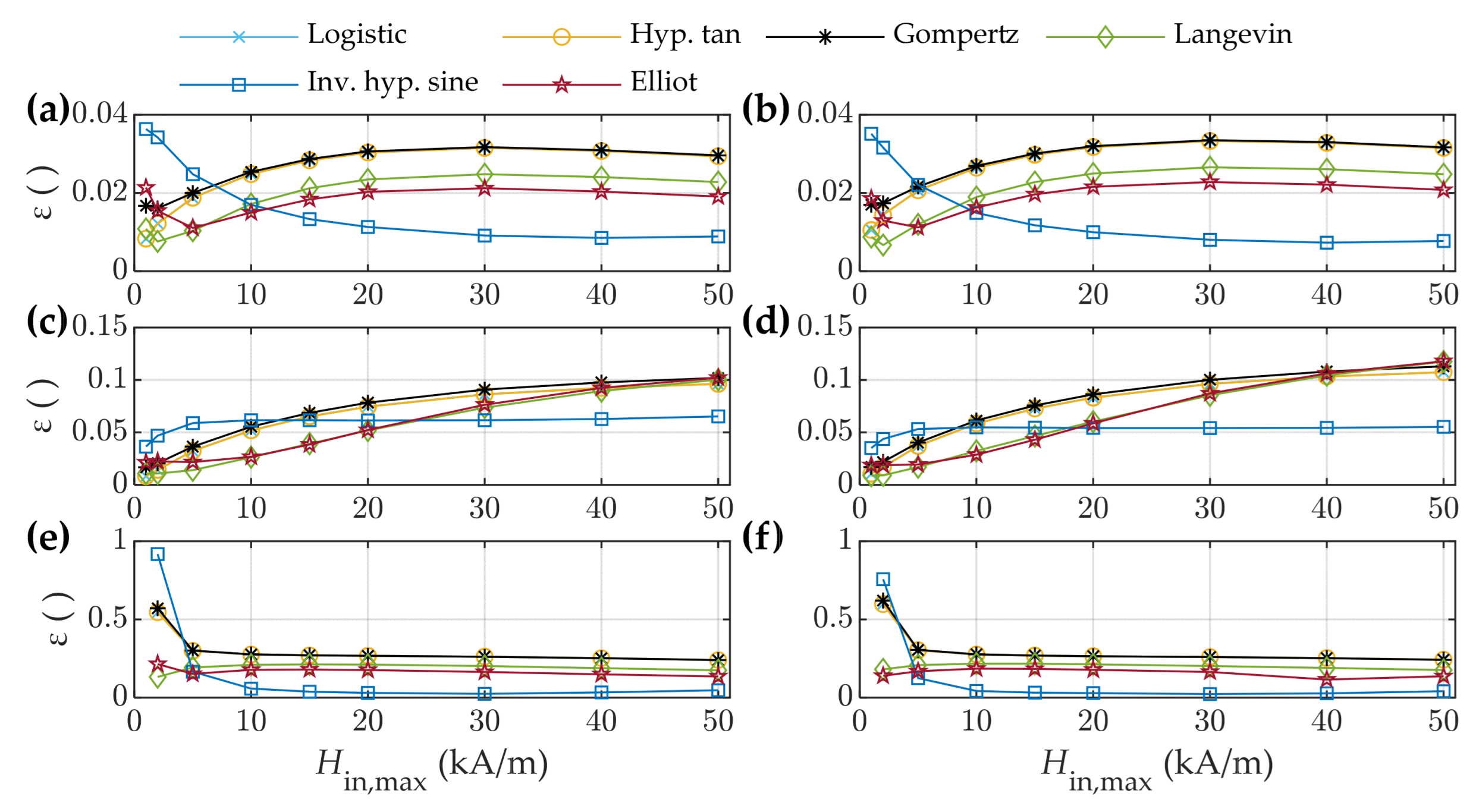
3.5. Evaluation of the Goodness of Fit

To evaluate the goodness of fit for the calculated curves, we applied the statistical measure normalized root mean square (NRMS) ε , defined by Equation (16) [7].
ε = 1 N m a x i = 1 N m a x J i n , i H e v a l , i J c a l c , i H e v a l , i Δ J e v a l 2
In Equation (16), J i n , i H e v a l , i are the measured values of magnetic polarization at corresponding magnetic field strengths H e v a l , i in the observed subregion for the evaluation of H e v a l . Furthermore, J c a l c , i H e v a l , i are the corresponding calculated values of magnetic polarization, and Δ J e v a l is the range of the evaluated subregion H e v a l . This range Δ J e v a l is defined as the difference between the maximum J e v a l , m a x and minimum J e v a l , m i n values of such a subregion, i.e., Δ J e v a l = J e v a l , m a x J e v a l , m i n .
During the analysis, we evaluated both the approximation and the extrapolation capabilities of the presented functions and curves. Individual curves were evaluated by Equation (16) in different subregions individually (i.e., HP, SAT, and EXT regions) by selecting the adequate evaluation region H e v a l .

3.5.1. Approximation Capabilities

We analyzed the goodness of fit and evaluated the approximation capabilities of the analytic functions and Bézier curves of different orders in specific subregions within the input subset H i n . The available measured data H m e a s were divided into nine input subsets H i n between H i n , m a x , H i n , m a x , where H i n , m a x equaled 1, 2, 5, 10, 15, 20, 30, 40, and 50 kA/m, respectively. An exemplary case of an input subset H i n , where H i n , m a x = 30 k A / m , is presented in Figure 4a with the blue curve. The first magnetization curves were fitted on the input subset H i n = 0 , H i n , m a x , whereas all the other curves were fitted on a symmetric subset H i n = H i n , m a x , H i n , m a x . In the first step, individual analytic functions were fitted, and Bézier curves of different orders were obtained for each individual input subset H i n . The evaluation of the goodness of fit ε was carried out in three subregions of each subset, where the evaluation was performed in the following ranges H e v a l ( H e v a l H i n ):
(a)
The input subset H e v a l , 1 = H i n = H i n , m a x , H i n , m a x ;
(b)
The HP subregion (within the input subset), i.e., H e v a l , 2 = H 1 , H 1 ;
(c)
The SAT region (within the input subset), i.e., H e v a l , 3 = H i n , m a x , H 1 H 1 , H i n , m a x .
The evaluation subregions H e v a l , 1 to H e v a l , 3 are depicted graphically in Figure 4a. It is important to note that J e v a l , m a x and J e v a l , m i n for case (c) were determined at H i n , m a x and H 1 , respectively.
The result of this analysis was the identification of the most suitable analytic functions and the most adequate orders of Bézier curves for the approximation of nonlinear magnetic properties for different input data subsets. These were included in the next analysis, i.e., the analysis of the extrapolation capabilities.

3.5.2. Extrapolation Capabilities

In the analysis of the extrapolation capabilities, the fitting was carried out analogously with the previous analysis. The difference was that the positive and negative saturation points J s H s were added to all symmetric input subsets between H i n , m a x , H i n , m a x . Therefore, the input subset H i n consisted of the negative saturation point H s , the measured data between H i n , m a x , H i n , m a x , and the positive saturation point H s , i.e., H i n = H s H i n , m a x , H i n , m a x H s . This input subset for a specific case, where H i n , m a x = 30   k A / m , is presented with the blue line and blue crosses in Figure 4b. The result of the fitting process was analytic functions and Bézier curves that ranged from H s to H s . They also enabled the analysis of the goodness of fit in the assumed EXT subregion. The evaluation of the goodness of fit ε was carried out again in three evaluation s u b r e g i o n s   H e v a l , where H e v a l H m e a s :
(d)
The full measured dataset up to saturation H e v a l , 4 = H m e a s ;
(e)
The subregion which contained the measured data H e v a l , 5 = H i n , m a x , H i n , m a x ;
(f)
The EXT subregion ( H e v a l , 6 = H s , H i n , m a x H i n , m a x , H s ).
Analogous to the previous subsection, J e v a l , m a x and J e v a l , m i n for case (f) were determined at H s and H i n , m a x , respectively.

4. Results

The available range (defined by H i n , m a x ) of the (measured) input data H i n = H i n , m a x , H i n , m a x has, in general, a high impact on the goodness of fit of the approximated functions and curves. The impact of the range on the approximated curves using both analytic functions and Bézier curves is presented in Figure 5. The curves in Figure 5a,b were approximated on the input subset limited by H i n , m a x = 0.5   k A / m and in Figure 5c,d on the input subset limited by H i n , m a x = 15   k A / m . The curves approximated on a bigger subset ( H i n , m a x = 15   k A / m ) deviated more in the HP region in comparison to those approximated on the input subset H i n , which coincided with the observed region ( H i n , m a x = 0.5   k A / m ). The approximated curves in Figure 5 confirm that the size of the input subset H i n (i.e., the range of measured input data defined by H i n , m a x ) had a high impact on the approximation accuracy.

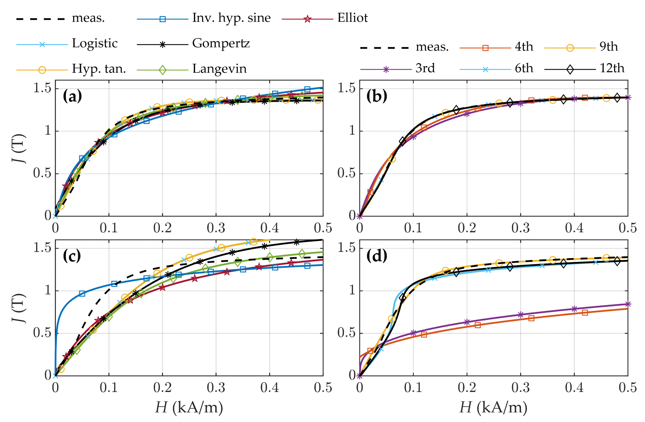
4.1. Approximation with Analytic Functions

In general, all analytic functions produced the overall shape to describe the discussed nonlinear relationships, as demonstrated, e.g., in Figure 5a,c. For the sigmoid functions (Functions (1)–(5)) similar conclusions are presented in [10,15].

4.1.1. Anhysteretic Curves

To determine the most adequate analytic function for the approximation of the anhysteretic curve, we calculated the NRMS deviations ε on different regions within different input subsets H i n for all the discussed functions, as described in Section 3.5.1. The obtained results are presented in Figure 6.
First, we evaluated the global goodness of fit (i.e., within different symmetric input subsets H e v a l , 1 = H i n of the measured data) systematically, as described in case (a) of Section 3.5.1. Based on the presented results in Figure 6a,b, it was observed that the Langevin function had the best overall fit for the smaller input subsets up to H i n , m a x = 5   k A / m . Further, the Elliot function had the best goodness of fit for the measured anhysteretic curve of both materials when a symmetric input subset from H i n , m a x = 5   k A / m up to H i n , m a x = 10   k A / m was applied. These results agree with the findings in [10]. The goodness of fit with the Langevin function was slightly worse compared to the one evaluated with the Elliot function in the latter region. However, if the input subsets exceeded H i n , m a x = 10   k A / m , the global goodness of fit of the inverse hyperbolic sine function was the best.
To support the obtained results further, we analyzed the deviations in two specific subregions of the anhysteretic curve. The first local goodness of fit was defined between H e v a l , 2 = H 1 , H 1 , where H 1 = 1   k A / m (the so-called HP region), as explained in case (b) of Section 3.5.1. The local goodness of fit for the HP region is shown in Figure 6c,d. The obtained results supported the premise that, as the input subset H i n increased into the saturation region, the deviations were more significant. This was expected due to the high nonlinearity of the input data, whereas individual subregions were not considered separately, and, consequently, could not be approximated with equal accuracy. In the HP region, the best results were again obtained using the Elliot and Langevin functions, whereas in the cases of larger input subsets above H i n , m a x = 20   k A / m , the inverse hyperbolic sine function again became the best option. If limited measured data not deep into saturation are available, the Elliot and Langevin functions are the best choice for approximation.
The second local subregion H e v a l , 3 (SAT region) was defined from 1   k A / m to the maximum value in the individual input subset H i n , m a x , i.e., when the materials were significantly saturated (i.e., case (c) in Section 3.5.1). The values of ε within this analysis are presented in Figure 6e,f. In this region the inverse hyperbolic sine function had superior results to other analytic functions, especially for input subsets that were measured deeper into saturation.

4.1.2. Major Loop Curves

Next, we analyzed the goodness of fit of the approximated analytic functions on the descending branch of the major loop. The calculated NRMS values ε are presented in Figure 7. The results obtained for the major loop are in line with those obtained for the anhysteretic curve. This could be attributed to the fact that the anhysteretic curve was calculated as the average value between both branches of the major loop, and, consequently, closely related to the major loop. It was concluded that the offset in H of the major loop curves did not introduce a significant change in the results.

4.1.3. First Magnetization Curves

The results obtained were slightly different in the case of the first magnetization curves. The calculated NRMS errors ε for the case of the first magnetization curve are shown in Figure 8. In the input subset between 0 and H i n , m a x , i.e., H i n = 0 , H i n , m a x , the Elliot and Langevin functions gave best results in the case of sheet NO35, as shown in Figure 8a. In the case of NO27, presented in Figure 8b, the Elliot and Langevin functions gave the best results up to H i n , m a x = 30   k A / m . Beyond this subregion, the inverse hyperbolic sine function became the most adequate analytic function. In the HP region, the Langevin function had the lowest deviation from the measured data in the case of NO35, as presented in Figure 8c. Figure 8d shows the results for NO27, where the Langevin function gave better results for the intermediate fields (up to H i n , m a x = 20   k A / m ), and, after that region, the Langevin and Elliot functions had similar goodness of fit. In the case of the SAT region (i.e., from 1 kA/m to H i n , m a x ), the results for both materials in Figure 8e,f were similar; overall, the inverse hyperbolic sine function yielded the best results. The Elliot and Langevin functions can be used for lower fields of up to H i n , m a x = 10   k A / m .

4.2. Approximation with Higher-Order Bézier Curves

Next, we analyzed the ability of Bézier curves of different orders systematically to describe the measured magnetization curves. We performed the analysis starting with Bézier curves of the order n = 3 (order three is commonly used in many applications, e.g., in splines [42]) and increased the order up to n = 12 .
Based on the results that are presented in Figure 5b,d we concluded that lower-order Bézier curves (e.g., the third and fourth orders) had limited ability to approximate magnetization curves adequately. Hence, we excluded these orders from further analysis. We applied the analysis presented in cases (a)–(c) in Section 3.5.1 to the approximation with Bézier curves.

4.2.1. Anhysteretic Curves

The obtained values of ε for the anhysteretic curves are presented in Figure 9. This part of the analysis was performed with Bézier curves from the 5th to 12th orders. For the sake of clarity, we did not plot ε for the Bézier curves of all the discussed orders but only representative ones. From the ε obtained for the individual symmetrical input subsets H e v a l , 1 = H i n (as explained in Section 3.5.1 case (a)) in Figure 9a,b, we concluded that the most suitable were the eighth- and ninth-order Bézier curves. In general, it is reasonable to select a curve with the lowest number of control points. The obtained results showed that all Bézier curves starting from order six already had significantly improved goodness of fit compared to the analytic functions in all the analyzed scenarios.
For the HP region (case (b) in Section 3.5.1) in Figure 9c,d, the ninth-order Bézier curve offered the best approximation, which is in line with the results in Figure 5b,d. Along with the 9th order, the 7th-, 8th-, and 10th-order Bézier curves yielded a very good approximation of this region. In this case, we observed that, as H i n increased, the fit in the HP region became less accurate, which was analogous with the results for the analytic functions. The same orders of Bézier curves were estimated as the best for the remaining SAT region of the curve (case (c) in Section 3.5.1) presented in Figure 9e,f.

4.2.2. Major Loop Curves

The results for the descending branch of the major loop are similar to the results obtained for the anhysteretic curve. The results are presented in Figure 10. The ninth-order Bézier curve had the lowest deviation from the measured major loop in all cases. The results obtained with the ninth-order curve were followed closely by the eighth-order Bézier curve.

4.2.3. First Magnetization Curves

In the case of approximating the first magnetization curve, Bézier curves were superior to analytic functions, whereas the obtained NRMS values ε were significantly lower. The calculated NRMS deviation values ε for the Bézier curves are presented in Figure 11. For this specific curve, even the fourth-order Bézier curve demonstrated low deviation from the measured data. For input subsets up to H i n , m a x = 30   k A / m , shown in Figure 11a,b, the sixth- and seventh-order Bézier curves yielded the best goodness of fit, and, above 30 kA/m, the eighth- and ninth-order Bézier curves yielded the best results. In the HP region, presented in Figure 11c,d, the seventh-order Bézier curve had the best overall goodness of fit. Those results are followed closely by the results obtained with the eighth-order Bézier curve. In the SAT region, presented in Figure 11e,f, the seventh-order Bézier curve had the best goodness of fit. Additionally, in the region with magnetic field strength values of up to H i n , m a x = 30   k A / m , the sixth-order Bézier curves demonstrated low deviation from the measured data. In regions with high magnetic field strength values beyond 30 kA/m, the eighth- and ninth-order Bézier curves had the lowest NRMS deviation values ε .
Based on the results in this subsection, we concluded that suitable orders of Bézier curves for approximation of the discussed nonlinear magnetic properties were the sixth to ninth.

4.3. Analysis of Extrapolation Capabilities

It is often not feasible to measure the hysteresis properties deep into saturation. Therefore, only measured magnetization curves in limited regions are available, as presented schematically in Figure 12a. The reasons for this are the highly nonlinear properties and the corresponding complexity and challenges in the measurement procedures. The measurement accuracy is decreased significantly when measurements are performed at values of high magnetic field strength H . Because of that, it is important to have a reliable method to determine the magnetic curves up to high saturation values, even if measured data are not available for the whole magnetization curve. This can be performed by extrapolation, which is the technique used most often for this purpose in applied engineering. Two of the most used functions for this purpose are the Langevin and the Elliot functions (the latter is often referred to as the Frölich–Kennelly extrapolation).
In Figure 12b, an example of limited available measured data is presented schematically. In such cases, a significant part of the magnetization curve is unknown and must be estimated with extrapolation. In the literature, several methods have been proposed for the extrapolation of magnetization curves [43]. Bézier curves could offer an additional reliable and good estimation of the extrapolated region of the magnetization curves if the saturation point is known. For that reason, we analyzed the capabilities of Bézier curves for the extrapolation of measured magnetic curve data and compared the results with the analytic functions. In this analysis, we included Bézier curves of the sixth to ninth orders, as well as the representative analytic functions, i.e., the Elliot, Langevin, and inverse hyperbolic sine functions. These were selected based on the results in Section 4.1 and Section 4.2.
The analysis was performed using input subsets H i n , and we assumed that the saturation point was known, i.e., we fixed the last point as the saturation point J s H s . Then, we shortened the input subset gradually. In this way, we could analyze the influence of the measured input subset’s size on the extrapolated part of the curve. The methodology is presented in Section 3.5.2 in cases (d)–(f). The measured and extrapolated curves of the NO27 electrical steel, where the input data were limited to the region between H i n , m a x , H i n , m a x , where H i n , m a x = 15   k A / m , are shown in Figure 13.

4.3.1. Anhysteretic Curves

First, we analyzed the goodness of fit for the full measured dataset of the anhysteretic curve, i.e., H e v a l , 4 = H m e a s (case (d) in Section 3.5.2). The goodness of fit for these regions is presented in Figure 14a,b. The eighth- and ninth-order Bézier curves had the best goodness of fit in the whole data range, followed closely by the seventh-order and sixth-order Bézier curves. The NRMS deviation ε became constant when the input subset reached a certain range. This range was approximately H i n , m a x = 20   k A / m for both discussed materials. As the H i n increased (and the extrapolation region decreased), ε decreased, which supports the conclusion from the previous analysis.
In the next step, we evaluated the deviations in two separate subregions of the approximated curves. The first was the subregion of the input data H e v a l , 5 = H i n , m a x , H i n , m a x , as described in Section 3.5.2 (e). The second was the EXT subregion, as presented in Section 3.5.2 (f). The goodness of fit for H e v a l , 5 is presented in Figure 14c,d, and for the EXT subregion H e v a l , 6 in Figure 14e,f. For both regions, the eighth- and ninth-order Bézier curves generated the lowest NRMS error ε and offered the best estimation of the measured curve. In both subregions, the inverse hyperbolic sine function had the lowest deviation from the measured data out of the chosen analytic functions and was comparable to the results obtained with the sixth-order Bézier curve.

4.3.2. Major Loop Curves

Figure 15 shows the calculated NRMS values ε obtained for the descending branch of the major loop. The conclusions are analogous to the analysis of the extrapolation of the anhysteretic curve. Overall, the eighth- and ninth-order Bézier curves offered the best goodness of fit, followed by the seventh-order Bézier curve. The sixth-order Bézier curve and the inverse hyperbolic sine function again had very similar results.

4.3.3. First Magnetization Curves

The results of the analysis of the first magnetization curve are presented in Figure 16. The Bézier curves again had superior results over the analytic functions in the case of the first magnetization curve. All orders from six to nine were suitable for the description of the first magnetization curve in all subsets and subregions in individual subsets. The results for the full region up to saturation are presented in Figure 16a,b, where the Bézier curves of orders seven to nine offered the best results. Slightly worse results were obtained using the sixth-order curve. In the region with the measured data (i.e., 0 , H i n , m a x   ) in Figure 16c,d, the results were in line with the full region. The extrapolation region in Figure 16e,f was the only region where one of the analytical functions, namely, the inverse hyperbolic sine function, came close to the accuracy of the Bézier curves. Among the Bézier curves, in the low-field-strength input datasets of up to H i n , m a x = 5   k A / m , the sixth-order Bézier curve had the lowest deviation, whereas in the more extended datasets, the seventh- to ninth-order Bézier curves again offered the best goodness of fit.

5. Discussion

Based on the results obtained within the performed analyses, the common takeaway is that both approaches, i.e., using adequate analytic functions or adequate Bézier curves, are suitable to describe or filter noisy measured data or extrapolate the nonlinear magnetic properties. Overall, Bézier curves of adequate orders (in most cases, between six and nine) offered significantly lower deviations from the measured curves compared with the analytic functions. The advantages and disadvantages of both approaches will be highlighted in this section.
Bézier curves are less sensitive to the size and range of the input dataset (limited by H i n , m a x ) than analytic functions. This is especially highlighted in Figure 9 and Figure 10, where it is shown that the Bézier curves had almost constant values of the NRMS deviation ε , whereas the Elliot function did not reach a constant value at different H i n , m a x . Further, as the order of Bézier curves increased (at a fixed maximum number of iterations of DE), starting from order nine, the goodness of fit became worse, which can be observed in Figure 9, Figure 10 and Figure 11 (order 12 had a higher NRMS deviation ε than order 9). Therefore, not all higher orders are adequate for approximating or extrapolating the measured subsets.
A downside of analytic functions is that their final point does not reach the saturation value. This property can be observed in Figure 13. They are limited by their mathematical description. It is possible to force the functions to go through the saturation point exactly but with the tradeoff of increasing the deviations in other subregions of the curve significantly, to the extent that the description in them is useless. A special and limiting feature of Bézier curves is that their starting points and endpoints can be fixed exactly without losing the agreement with the measured data in any region (i.e., the first and last control points are interpolated, whereas the intermediate points are used to manipulate the shape and curvature of the curve). Furthermore, Bézier curves allow the slope at which the curve approaches saturation to be prescribed, as explained in Section 2.2.1. This can be both an advantage and a disadvantage. For example, a very accurate extrapolation is possible only when the saturation point of the material is known (e.g., can be calculated or estimated theoretically).
The straightforward calculation of derivatives in any point of the curve and, consequently, the curvature of the curve, allows for the precise determination of the shape of a curve under construction. Measured magnetic curves can have a lot of noise in the HP region as the maximum value of magnetic field density increases. Bézier curves have the potential to make the extraction of measured data easier. The user could set the theoretically known saturation value, the slope at which the saturation is reached, and the curvature in individual regions to obtain a symmetrical curve and, consequently, a symmetrical loop. In this way, the potential non-physical behavior of the obtained curves can be avoided (similar to the behavior of the curves in Figure 5b,d). In this work, the only prescribed limitation was not to exceed the value of magnetic polarization at saturation J s H s , i.e., the control points could have been placed anywhere below that point (and above the negative saturation J s H s ). Additionally, pairwise symmetrical control points can be prescribed during the DE calculation to obtain symmetrical Bézier curves [40].

6. Conclusions

From the obtained results, we concluded that Bézier curves are promising candidates to adequately model the nonlinear properties of NO soft magnetic materials. Through the flexibility of curve order and adequate placement of control points, Bézier curves can approximate the shape of the magnetization curves with significantly lower deviation compared to analytic functions.
With the performed analysis, we concluded that Bézier curves from order six and higher are suitable for the approximation of the discussed magnetization curves. The approximation with those orders offers significantly improved fit based on the measured data compared with approximations with all the discussed analytic functions. In our specific case, the ninth order Bézier curve offered the best goodness of fit in all the analyzed subregions.
Bézier curves can approximate the high saturation region accurately (i.e., the extrapolation region). However, the theoretical point of saturation is required, in addition to the measurements in the HP subregion. To achieve high accuracy, it would be necessary to prescribe further boundary conditions at which the curve is generated. Examples are prescribing the slope for reaching the saturation region and adjusting the smoothness of the curvature along individual segments of the magnetization curve while calculating the control points. Our future work will focus on analyzing the conditions to generate symmetrical and accurate magnetization curves.

Author Contributions

Conceptualization, E.R. and M.P.; methodology, E.R. and M.P.; software, E.R.; validation, E.R.; formal analysis, E.R.; investigation, E.R.; resources, E.R.; data curation, E.R.; writing—original draft preparation, E.R.; writing—review and editing, E.R. and M.P.; visualization, E.R.; supervision, M.P.; project administration, M.P.; funding acquisition, M.P. All authors have read and agreed to the published version of the manuscript.

Funding

This research was funded by the Slovenian Research and Innovation Agency (ARIS) under grant numbers J7-3152 and P2-0115.

Data Availability Statement

Data available on request.

Conflicts of Interest

The authors declare no conflicts of interest.

References

  1. Tellinen, J. A simple scalar model for magnetic hysteresis. IEEE Trans. Magn. 1998, 34, 2200–2206. [Google Scholar] [CrossRef]
  2. Zirka, S.E.; Moroz, Y.I.; Harrison, R.G.; Chiesa, N. Inverse Hysteresis Models for Transient Simulation. IEEE Trans. Power Deliv. 2014, 29, 552–559. [Google Scholar] [CrossRef]
  3. Vo, A.-T.; Fassenet, M.; Préault, V.; Espanet, C.; Kedous-Lebouc, A. New formulation of Loss-Surface Model for accurate iron loss modeling at extreme flux density and flux variation: Experimental analysis and test on a high-speed PMSM. J. Magn. Magn. Mater. 2022, 563, 169935. [Google Scholar] [CrossRef]
  4. Kokornaczyk, E.; Gutowski, M.W. Anhysteretic Functions for the Jiles–Atherton Model. IEEE Trans. Magn. 2015, 51, 1–5. [Google Scholar] [CrossRef]
  5. Yang, J.; Shi, M.; Zhang, X.; Ma, Y.; Liu, Y.; Yuan, S.; Han, B. Demagnetization Parameters Evaluation of Magnetic Shields Based on Anhysteretic Magnetization Curve. Materials 2023, 16, 5238. [Google Scholar] [CrossRef] [PubMed]
  6. Mörée, G.; Leijon, M. Review of Hysteresis Models for Magnetic Materials. Energies 2023, 16, 3908. [Google Scholar] [CrossRef]
  7. Steentjes, S.; Hameyer, K.; Dolinar, D.; Petrun, M. Iron-Loss and Magnetic Hysteresis Under Arbitrary Waveforms in NO Electrical Steel: A Comparative Study of Hysteresis Models. IEEE Trans. Ind. Electron. 2017, 64, 2511–2521. [Google Scholar] [CrossRef]
  8. Bertotti, G. Hysteresis in Magnetism: For Physicists, Materials Scientists, and Engineers; Academic Press: Cambridge, MA, USA, 1998. [Google Scholar]
  9. Takács, J. A phenomenological mathematical model of hysteresis. Compel 2001, 20, 1002–1014. [Google Scholar] [CrossRef]
  10. Jesenik, M.; Mernik, M.; Trlep, M. Determination of a Hysteresis Model Parameters with the Use of Different Evolutionary Methods for an Innovative Hysteresis Model. Mathematics 2020, 8, 201. [Google Scholar] [CrossRef]
  11. Hofmann, M.J.; Herzog, H.-G. Modeling Magnetic Power Losses in Electrical Steel Sheets in Respect of Arbitrary Alternating Induction Waveforms: Theoretical Considerations and Model Synthesis. IEEE Trans. Magn. 2015, 51, 1–11. [Google Scholar] [CrossRef]
  12. Bastos, J.P.A.; Hoffmann, K.; Leite, J.V.; Sadowski, N. A New and Robust Hysteresis Modeling Based on Simple Equations. IEEE Trans. Magn. 2018, 54, 1–4. [Google Scholar] [CrossRef]
  13. Messal, O.; Vo, A.T.; Fassenet, M.; Mas, P.; Buffat, S.; Kedous-Lebouc, A. Advanced approach for static part of loss-surface iron loss model. J. Magn. Magn. Mater. 2020, 502, 166401. [Google Scholar] [CrossRef]
  14. Szczyglowski, J. Use of quasi-static loops of magnetic hysteresis in loss prediction in non-oriented electrical steels. Physica B 2020, 580, 411812. [Google Scholar] [CrossRef]
  15. Petrescu, L.; Cazacu, E.; Petrescu, C. Sigmoid functions used in hysteresis phenomenon modeling. In Proceedings of the 2015 9th International Symposium on Advanced Topics in Electrical Engineering (ATEE), Bucharest, Romania, 7–9 May 2015. [Google Scholar] [CrossRef]
  16. Li, Q.; Li, J.-P.; Chen, L. A Bezier Curve-Based Font Generation Algorithm for Character Fonts. In Proceedings of the 2018 IEEE 20th International Conference on High Performance Computing and Communications; IEEE 16th International Conference on Smart City; IEEE 4th International Conference on Data Science and Systems (HPCC/SmartCity/DSS), Exeter, UK, 28–30 June 2018. [Google Scholar] [CrossRef]
  17. Amat, N.F.I.C.; Yahya, Z.R.; Rusdi, N.A.; Helmee, N.A.; Muhamadd, W.Z.A.W. Arabic Fonts Representation in Cubic Bézier Curve using Different Soft Computing Algorithm. IOP Conf. Ser. Mater. Sci. Eng. 2019, 705, 012026. [Google Scholar] [CrossRef]
  18. Vinayak, A.; Zakaria, M.A.; Baarath, K.; Majeed, A.P.P.A. A novel Bezier curve control point search algorithm for autonomous navigation using N-order polynomial search with boundary conditions. In Proceedings of the 2021 IEEE International Intelligent Transportation Systems Conference (ITSC), Indianapolis, IN, USA, 19–22 September 2021. [Google Scholar] [CrossRef]
  19. Choi, J.-W.; Curry, R.; Elkaim, G. Path Planning Based on Bezier Curve for Autonomous Ground Vehicles. In Proceedings of the Advances in Electrical and Electronics Engineering—IAENG Special Edition of the World Congress on Engineering and Computer Science 2008, San Francisco, CA, USA, 22–24 October 2008. [Google Scholar] [CrossRef]
  20. Han, L.; Yashiro, H.; Tehrani Nik Nejad, H.; Do, Q.H.; Mita, S. Bezier curve based path planning for autonomous vehicle in urban environment. In Proceedings of the 2010 IEEE Intelligent Vehicles Symposium, La Jolla, CA, USA, 21–24 June 2010. [Google Scholar] [CrossRef]
  21. Satai, H.A.; Zahra, M.M.A.; Rasool, Z.I.; Abd-Ali, R.S.; Pruncu, C.I. Bézier Curves-Based Optimal Trajectory Design for Multirotor UAVs with Any-Angle Pathfinding Algorithms. Sensors 2021, 21, 2460. [Google Scholar] [CrossRef]
  22. Coskun, O.; Turkmen, H.S. Multi-objective optimization of variable stiffness laminated plates modeled using Bezier curves. Compos. Struct. 2022, 279, 114814. [Google Scholar] [CrossRef]
  23. Nuntawisuttiwong, T.; Dejdumrong, N. An Approximation of Bézier Curves by a Sequence of Circular Arcs. Inf. Technol. Control 2021, 50, 213–223. [Google Scholar] [CrossRef]
  24. Tiismus, H.; Kallaste, A.; Vaimann, T.; Lind, L.; Virro, I.; Rassõlkin, A.; Dedova, T. Laser Additively Manufactured Magnetic Core Design and Process for Electrical Machine Applications. Energies 2022, 15, 3665. [Google Scholar] [CrossRef]
  25. Hussain, S.; Kallaste, A.; Vaimann, T. Recent Trends in Additive Manufacturing and Topology Optimization of Reluctance Machines. Energies 2023, 16, 3840. [Google Scholar] [CrossRef]
  26. Matwankar, C.S.; Pramanick, S.; Singh, B. Flux-linkage Characterization and Rotor Position Estimation of Switched Reluctance Motor using Bézier Curves. In Proceedings of the 2021 IEEE 2nd International Conference on Smart Technologies for Power, Energy and Control (STPEC), Bilaspur, India, 19–22 December 2021. [Google Scholar] [CrossRef]
  27. Louzazni, M.; Al-Dahidi, S. Approximation of photovoltaic characteristics curves using Bezier Curve. Renew. Energy 2021, 174, 715–732. [Google Scholar] [CrossRef]
  28. Shi, N.; Lv, Y.L.; Zhang, Y.C.; Zhu, X.H. Linear fitting Rule of I-V characteristics of thin-film cells based on Bezier function. Energy 2023, 278, 127997. [Google Scholar] [CrossRef]
  29. Cui, X.; Li, Y.; Xu, L. Adaptive Extension Fitting Scheme: An Effective Curve Approximation Method Using Piecewise Bézier Technology. IEEE Access 2023, 11, 58422–58435. [Google Scholar] [CrossRef]
  30. Said Mad Zain, S.A.A.A.; Misro, M.Y.; Miura, K.T. Generalized Fractional Bézier Curve with Shape Parameters. Mathematics 2021, 9, 2141. [Google Scholar] [CrossRef]
  31. Rahmanović, E.; Petrun, M. Approximation of nonlinear properties of soft-magnetic materials with Bézier curves. In Proceedings of the 2023 IEEE International Magnetic Conference—Short Papers (INTERMAG Short Papers), Sendai, Japan, 15–19 May 2023. [Google Scholar] [CrossRef]
  32. Steentjes, S.; Petrun, M.; Glehn, G.; Dolinar, D.; Hameyer, K. Suitability of the double Langevin function for description of anhysteretic magnetization curves in NO and GO electrical steel grades. AIP Adv. 2017, 7, 056013. [Google Scholar] [CrossRef]
  33. Skarlatos, A.; Theodoulidis, T. A Modal Approach for the Solution of the Non-Linear Induction Problem in Ferromagnetic Media. IEEE Trans. Magn. 2016, 52, 1–11. [Google Scholar] [CrossRef]
  34. Baydas, S.; Karakas, B. Defining a curve as a Bezier curve. J. Taibah Univ. Sci. 2019, 13, 522–528. [Google Scholar] [CrossRef]
  35. Ezhov, N.; Neitzel, F.; Petrovic, S. Spline Approximation, Part 2: From Polynomials in the Monomial Basis to B-splines—A Derivation. Mathematics 2021, 9, 2198. [Google Scholar] [CrossRef]
  36. Kiliçoglu, Ş.; Şenyurt, S. On the matrix representation of 5th order Bézier Curve and derivatives in E^3. Commun. Fac. Sci. Univ. Ank. Ser. A1 Math. Stat. 2022, 71, 133–152. [Google Scholar] [CrossRef]
  37. Kilicoglu, S.; Yurttancikmaz, S. How to approximate cosine curve with 4th and 6th order Bezier curve in plane? Therm. Sci. 2022, 26, 559–570. [Google Scholar] [CrossRef]
  38. Rovenski, V. Piecewise Curves and Surfaces. In Modeling of Curves and Surfaces with MATLAB®; Springer: New York, NY, USA, 2010; pp. 357–411. [Google Scholar]
  39. Pijls, H.; Quan, L.P. A Computational Method with Maple for Finding the Maximum Curvature of a Bézier-Spline Curve. Math. Comput. Appl. 2023, 28, 56. [Google Scholar] [CrossRef]
  40. Sanchez-Reyes, J. Detecting symmetries in polynomial Bezier curves. J Comput Appl Math 2015, 288, 274–283. [Google Scholar] [CrossRef]
  41. Pandunata, P.; Shamsuddin, S.M.H. Differential Evolution Optimization for Bezier Curve Fitting. In Proceedings of the 2010 Seventh International Conference on Computer Graphics, Imaging and Visualization, Sydney, Australia, 7–10 August 2010. [Google Scholar] [CrossRef]
  42. Ezhov, N.; Neitzel, F.; Petrovic, S. Spline approximation, Part 1: Basic methodology. J. Appl. Geod. 2018, 12, 139–155. [Google Scholar] [CrossRef]
  43. Wang, L.; Ding, F.; Yang, D.; Wang, K.; Jiao, B.; Chen, Q. A fitting-extrapolation method of B-H curve for magnetic saturation applications. COMPEL Int. J. Comput. Math. Electr. Electron. Eng. 2023, 42, 494–505. [Google Scholar] [CrossRef]
Figure 1. Graphical presentation and comparison of the analyzed mathematical functions.
Mathematics 12 00445 g001
Figure 2. Various shapes formed with Bézier curves of different orders: (a) n = 3, (b) n = 3, (c) n = 5, and (d) n = 10.
Mathematics 12 00445 g002
Figure 3. Impact of the placement of control points P 1 and P 2 on the shape of a 3rd-order Bézier curve: (a,b) changing the curvature and slope of a single valued curve, (c) overshoot over normalized value of 1 (d) non single valued curve.
Mathematics 12 00445 g003
Figure 4. Graphic presentation of the input subsets of measured data H i n and characteristic subregions for evaluation of the goodness of fit ( H e v a l , 1 to H e v a l , 6 ) in the cases of (a) approximation and (b) extrapolation.
Mathematics 12 00445 g004
Figure 5. Impact of the range of measured data H i n , m a x on the goodness of fit in the region 0 ,   0.5   k A / m : (a) analytic functions, H i n , m a x = 0.5   k A / m ; (b) Bézier curves of different orders, H i n , m a x = 0.5   k A / m ; (c) analytic functions, H i n , m a x = 15   k A / m ; and (d) Bézier curves of different orders, H i n , m a x = 15   k A / m .
Mathematics 12 00445 g005
Figure 6. Calculated NRMS deviation ε within the individual input subsets H i n = H i n , m a x , H i n , m a x for the anhysteretic curve of two materials NO35 (left column) and NO27 (right column) approximated with analytic functions (a,b) within the individual input subsets H i n , (c,d) within the HP subregion of the individual subsets, and (e,f) within the SAT subregion of the individual subsets.
Mathematics 12 00445 g006
Figure 7. Calculated NRMS deviation ε within the individual input subsets H i n = H i n , m a x , H i n , m a x for the descending branch of the major loop of two materials, NO35 (left column) and NO27 (right column), approximated with analytic functions (a,b) within the individual input subsets H i n , (c,d) within the HP subregion of the individual subsets, and (e,f) within the SAT subregion of the individual subsets.
Mathematics 12 00445 g007
Figure 8. Calculated NRMS deviation ε within the individual input subsets H i n = H i n , m a x , H i n , m a x for the first magnetization curve of two materials, NO35 (left column) and NO27 (right column), approximated with analytic functions (a,b) within the individual input subsets H i n between 0 and H i n , m a x , (c,d) within the HP subregion between 0 and 1 kA/m of the individual subsets, and (e,f) within the SAT subregion between 1 kA/m and H i n , m a x of the individual subsets.
Mathematics 12 00445 g008
Figure 9. Calculated NRMS deviation ε within the individual input subsets H i n = H i n , m a x , H i n , m a x for the anhysteretic curves of two materials, NO35 (left column) and NO27 (right column), approximated with Bézier curves (a,b) within the individual input subsets H i n , (c,d) within the HP subregion of the individual subsets, and (e,f) within the SAT subregion of the individual subsets.
Mathematics 12 00445 g009
Figure 10. Calculated NRMS deviation ε within the individual input subsets H i n = H i n , m a x , H i n , m a x for the descending branch of the major loop of two materials, NO35 (left column) and NO27 (right column), approximated with Bézier curves: (a,b) within the individual input subsets H i n , (c,d) within the HP subregion of the individual subsets, and (e,f) within the SAT subregion of the individual subsets.
Mathematics 12 00445 g010
Figure 11. Calculated NRMS deviation ε within the individual input subsets H i n = H i n , m a x , H i n , m a x for the first magnetization curve of two materials, NO35 (left column) and NO27 (right column), approximated with Bézier curves (a,b) within the individual input subsets H i n between 0 and H i n , m a x , (c,d) within the HP subregion between 0 and 1 kA/m of the individual subsets, and (e,f) within the SAT subregion between 1 kA/m and H i n , m a x of the individual subsets.
Mathematics 12 00445 g011
Figure 12. (a) Anhysteretic curve in the HP region and (b) anhysteretic curve measured up to saturation.
Mathematics 12 00445 g012
Figure 13. Extrapolation region for the anhysteretic curve with Bézier curves and analytic functions in the case where the input data were limited to the region between 15 ,   15   k A / m .
Mathematics 12 00445 g013
Figure 14. Calculated NRMS deviation ε within the individual input subsets H i n = H s H i n , m a x , H i n , m a x H s for the anhysteretic curve of two materials, NO35 (left column) and NO27 (right column), approximated with Bézier curves and analytic functions, including extrapolation (a,b) within the measured dataset H e v a l , 4 = H m e a s , (c,d) within the subregion H e v a l , 5 = H i n , m a x , H i n , m a x of the individual subsets, and (e,f) within the EXT subregion H e v a l , 6 of the individual subsets.
Mathematics 12 00445 g014
Figure 15. Calculated NRMS deviation ε within the individual input subsets H i n = H s H i n , m a x , H i n , m a x H s for the descending branch of the major loop of two materials, NO35 (left column) and NO27 (right column), approximated with Bézier curves and analytic functions, including extrapolation (a,b) within the measured dataset H e v a l , 4 = H m e a s , (c,d) within the subregion H e v a l , 5 = H i n , m a x , H i n , m a x of the individual subsets, and (e,f) within the EXT subregion H e v a l , 6 of the individual subsets.
Mathematics 12 00445 g015
Figure 16. Calculated NRMS deviation ε within the individual input subsets H i n = H s H i n , m a x , H i n , m a x H s for the first magnetization curve of two materials, NO35 (left column) and NO27 (right column), approximated with Bézier curves and analytic functions, including extrapolation (a,b) within the measured dataset between 0 and H s , (c,d) within the subregion between 0 and H i n , m a x of the individual subsets, and (e,f) within the EXT subregion between H i n , m a x and H s of the individual subsets.
Mathematics 12 00445 g016
Table 1. Mathematical equations of selected analytic functions.
Analytic FunctionEquation
Logistic 2 a d + e b x c a (1)
Hyperbolic tangent a · tanh b · x + c (2)
Elliot a · x + c d + b · x + c (3)
Gompertz 2 a · e e b x c a (4)
Langevin a · coth x + c b b x + c (5)
Inverse hyperbolic sine a · asinh b · x + c (6)
Disclaimer/Publisher’s Note: The statements, opinions and data contained in all publications are solely those of the individual author(s) and contributor(s) and not of MDPI and/or the editor(s). MDPI and/or the editor(s) disclaim responsibility for any injury to people or property resulting from any ideas, methods, instructions or products referred to in the content.

