1. Introduction
The (human user) comfort and optimal use of energy are two elements that must be considered for the design of any vehicle. Optimal energy use is especially relevant as there is a wide consensus that unnecessary thermal contamination degrades the environment and that for any electrical vehicle, the use of energy should be optimal. To optimize both of these aspects, suitable suspension elements must be used. Vehicle suspensions are characterized by a set of parameters such as the relevant masses, stiffness of the springs, and the damping of the shock absorbers, all of which characterize a vehicle’s dynamic behavior.
The accurate identification of these dynamic parameters in vehicle suspension systems is of paramount importance in the automotive industry, serving not only for design and optimization but also as a critical factor in ensuring vehicle safety and operational efficiency. Data acquisition availability and analysis techniques have fostered new methodologies for parameter identification, utilizing synthetic or experimental data. This approach circumvents the traditionally invasive and time-consuming process of physical disassembly of suspension parameters when a dynamic suspension model is needed, presenting several compelling advantages.
Avoiding the labor-intensive process of physical testing significantly reduces both the time and financial resources required for suspension analysis and optimization. It enables the evaluation of suspension performance under actual driving conditions, providing a more accurate reflection of in-service vehicle behavior. Such capabilities facilitate the fine-tuning of suspension systems for improved ride comfort, vehicle stability, and energy efficiency without reliance on extensive physical prototyping.
Streamlining the maintenance process and diagnosis of suspension issues leads to more effective and timely interventions. It also contributes to the creation of more precise models for vehicle dynamics simulation and analysis, essential for ongoing research and development. This approach supports the development and implementation of sophisticated suspension control systems, including adaptive and semi-active suspensions.
Moreover, a quick method to monitor the condition of suspension parameters over time offers the potential for predicting failures, ensuring that vehicles remain within the safety standards set by manufacturers. It also provides a method for quick testing in vehicle inspection stations to verify if the vehicle dynamics meet the required standards or to identify any deficiencies.
This manuscript presents an easy-to-implement methodology to identify a vehicle’s suspension parameters from the dynamic behavior of the vehicle when it faces different external actions. Based on this dynamic data (coming from mathematical, synthetic data, or from experimental data), the proposed methodology studies the kinematic behavior of the suspension to extract and identify the dynamic data (masses, rigidity, and damping) from such suspension. Therefore, this study focuses on rapid parameter identification from non-destructive and non-invasive data sources, which is not just an academic pursuit, but also addresses a practical necessity in the automotive industry. It underscores the need for efficient, accurate, and cost-effective methods to ensure vehicle safety, performance, and compliance with evolving standards.
To compare this approach, an analysis of the state-of-the-art in vehicle suspension parameter identification is presented, integrating both experimental and theoretical approaches. It encompasses a diversity of methodologies, ranging from basic local optimization to advanced techniques like Kalman filters, adaptive observers, and neural networks. It highlights works that utilize models from quarter-vehicle to half-vehicle (bicycle) models, including research on active and semi-active suspensions, adaptive control systems, and driver and passenger comfort analysis. The relevance of parameter variability, such as stiffness and damping, response to road perturbations like speed bumps and curbs, and the inclusion of noise in the data, are common themes in the reviewed studies.
Parameter identification is, thus, one topic of special interest for any mobility-related engineering task. Far from being a closed subject, new research is being carried out in this area. In Ref. [
1], for instance, Vyasarayani et al. recognized that the essential nature of parameter identification was an optimization problem, and they proposed a new method based on homotopy aimed at finding the global minima, pointing out that some deterministic methods usually find the local minima.
In Ref. [
2], a method based on a mutual information metric was proposed by Sujan and Dubowsky, where the core of the mathematical model is a Newton–Euler one and the solving of the dynamic parameters is carried out via a Kalman filter. In Ref. [
3], Weispfenning used a procedure based on neural networks.
In Ref. [
4], Imine and Madani developed a method for a heavy vehicle based on the sliding mode observer coupled with a Lagrangian formulation of the dynamical problem, whereas in Ref. [
5], Hong et al. developed a method based on a Dual Unscented Kalman Filter for a four-wheel vehicle model.
In Ref. [
6], Wang et al. developed a system focused on the truck driver and seating system whose parameters were identified. This kind of research is of the utmost importance because the human driver and passengers can feel comfortable under a restricted frequency interval. Likewise, in Ref. [
7], Sun et al. applied parameter identification when they developed a variable stiffness and damping shock absorber—thus, we are talking about a semi-active vehicle suspension—where both damping and stiffness variability are tested, the frequency response is analyzed, and the parameters are identified.
In Ref. [
8], in a work by Lauß et al., the discrete adjoint method was presented and applied to an engine mount, where the focus, again, was on the particular approach for solving the set of differential equations—now enlarged—and thus, obtaining the parameters under consideration. The use of the Levenberg–Marquardt parameter estimation algorithm was applied to a four-degrees-of-freedom (DOF), non-linear motorcycle model in Ref. [
9], by Fouka et al.
Sun et al. studied a non-linear ball-screw inerter. Here, the influence of the non-linearities of the ball-screw inerter were analyzed and compared with those of a linear inerter [
10]. The model used was a three-passive-suspension layout half-car one, where the parameters are found via the recursive least-squares algorithm based on test data.
Active suspension models were studied in [
11] where a Local Linear Model tree (LOLIMOT), a special neural network architecture was used to ascertain the suspension parameters by Fischer et al. Buggaveeti, in her master’s thesis [
12], using the concept of Model-Based-Design (MBD), developed a validated vehicle dynamics model for a Toyota Prius Plug-in hybrid vehicle. Both a local optimization algorithm and homotopy, which is a global optimization technique were used and compared.
Rajamani and Hedrick developed an adaptive observer [
13], for an active suspension system. Kogut, in turn, used a grey-box model identification technique for a semi-active suspension system composed of a non-linear two-DOF mass-coupled system with a magnetorheological (MR) rotary damper [
14].
In the book [
15], in the Parallel Strand II Virtual Development Methods, further analysis can be seen using Artificial Neural Networks such as in [
16], using virtual prototypes [
17], and analyzing passive vehicle dynamics concentrating the research in active safety and, quite importantly, in autonomous driving [
18].
The research carried out by Sarmah and Tiwari in which a cracked rotor system equipped with active magnetic bearings was studied, starting from a physical model, is also noteworthy [
19].
Callejo and de Jalón delved into theoretical considerations focusing on the sensitivity of the system of interest. This paper is more general in nature than the previous ones [
20].
Akar and Dere developed a real-time adaptive switching controller whose purpose was to mitigate rollover accidents without reducing the performance of the vehicle. The core of the system relies on “adaptive identification of vehicle lateral and vertical dynamics parameters, including the center-of-gravity height that has a major role in rollover”. The least-squares and the Kalman filtering techniques were used from a computational point of view [
21].
However, Best M.C. concentrated on the modelling requirements if one is to implement in a practical way an advanced vehicle suspension control system [
22], while Serban and Freeman delved into parameter estimation for multibody dynamic systems using Levenberg-Marquardt methods. Again, in this article, the dichotomy between global and local methods is raised [
23].
In Metallidis et al.’s work, a methodology for ascertaining the optimal sensor location and configuration was proposed, starting with the classic two-DOF, quarter-car model, and finally raising the complexity to four-wheel vehicles with flexible bodies [
24].
Hahn et al., using a differential global positioning system, succeeded in the estimation of the road–tire friction coefficient, showing that these types of sensors can provide enough information for estimating these parameters [
25], whereas Elsawaf et al. developed a method for identifying the parameters of a magnetorheological damper using the particle swarm optimization [
26]. Alfi and Fateh used a modified particle swarm optimization for a non-linear system, namely, a hydraulic suspension system [
27].
Zhao et al. modeled a heavy truck with a three-DOF cabin linear system model using a bench test [
28], while Roy and Liu [
29] analyzed the road vehicle suspension and performance evaluation using an eight-DOF, two-dimensional vehicle model simulating and animating the response of a vehicle under “different road, traction, braking and wind conditions”.
Ma et al.’s work is of special interest to this paper due to them using an inverse model to improve the performance of vehicle suspension, proposing a semi-active vehicle suspension with a magnetorheological fluid (MRF) damper [
30].
Finally, Rodríguez et al., using a dual Kalman filter composed by an errorEKF and an unscented Kalman filter following the multibody dynamics approach, obtained a model with a high level of detail including non-linear dynamics [
31].
In contrast to the diverse methodologies outlined in the state-of-the-art, this paper introduces a novel approach for vehicle suspension parameter identification that concentrates on the analysis of the position and the velocity signals from both the suspended and the unsuspended masses of a vehicle’s suspension system. These position and velocity signals can be obtained from the suspension dynamic’s mathematical equations (see the different suspension models and equations in
Section 2) and from data acquisition in sensorized vehicle suspensions. In the latter, acquisition errors and deviations can be present. This is why the proposed methodology includes an analysis of errors (externally added) even in the case of the mathematical synthetic (clean) data from the equations. While existing research predominantly focuses on a variety of optimization and estimation techniques, such as Kalman filters, neural networks, and adaptive control systems, the methodology proposed here uniquely advances the suspension dynamics analysis by not only developing a methodology and a mathematical tool for parameter identification but also through a detailed exploration of the global approach.
At the core of the methodology is the application of dynamic equations of vehicle suspension. Beginning with initially unknown parameters, we iteratively modify the dynamic curves of the suspension, tracking deviations at fixed time intervals against the baseline signals. A fundamental element of this approach is the use of a basic optimization algorithm, the Nelder–Mead algorithm (NM algorithm), aimed at predicting the optimal parameters that minimize the overall signal errors. This algorithm is famed for its derivative-free approach and is adept at handling complex, non-linear functions like those involved in vehicle suspension dynamics. Its simplicity in implementation is a significant advantage, especially when dealing with intricate systems. While it does have limitations, such as potential slow convergence and sensitivity to initial parameters, its robustness in dealing with functions that may exhibit noise (such as the ones obtained from vehicle sensorization) or discontinuities makes it a compelling option for this specific application. This method, with its flexibility and ease of use, can effectively be integrated into the challenges of this parameter identification problem.
The selection of the Nelder–Mead algorithm for this study is primarily motivated by its fundamental properties and limitations. As a local optimization algorithm, Nelder–Mead is adept at finding local minima of mathematical functions, but it does not guarantee global convergence as the more comprehensive global optimization algorithms do. This characteristic presents a unique opportunity for this investigation. The aim is to ascertain whether such a basic, local optimization algorithm is sufficient for accurately identifying vehicle suspension parameters from synthetic data. By testing the efficacy of the Nelder–Mead algorithm in this constrained setting, it is possible to establish a foundational understanding of the parameter identification process. This approach serves as an initial step before considering more complex and globally convergent algorithms. Such a progression is crucial for determining the necessary computational complexity and robustness required for effective suspension parameter identification in various scenarios.
The main contribution of this study lies in the introduction of a straightforward and scalable methodology for suspension parameter identification within complex simultaneous dynamic equations, considering the use of position and velocity signals from both suspended and unsuspended masses across various suspension models. This methodology is designed to encompass parameter identification from both mathematically synthetic signals and from signals with inherent noise in sensorized suspensions. The chosen algorithm for this purpose is based on Nelder–Mead, facilitating the discretization of signals while providing a simple yet robust method for multi-parameter optimization. This algorithm is used for iteratively adjusting dynamic suspension curves against baseline signals, allowing for the more focused and precise identification of optimal suspension parameters. Our approach represents a significant advancement in suspension dynamics analysis, offering a comprehensive and innovative tool for minimizing signal errors in suspension parameter identification, even under noisy data.
This study methodically tests the proposed methodology across theoretical vehicle models of increasing complexity. It starts with a quarter-vehicle suspension model with one degree of freedom, advances to a two-degrees-of-freedom model, and ultimately applies the methodology to a half-vehicle (motorcycle) model. For each of these models, the results are obtained and analyzed to evaluate the effectiveness, limitations, and scope of the proposed methodology. Furthermore, potential improvements are discussed, and the application of this methodology to a future, highly non-linear full-vehicle model, integrating the insights and enhancements identified in this article is envisioned.
2. Framework
The main objective of the present research is centered on the characteristic suspension parameters at a theoretical level. Specifically, of special interest are the conditions under which accurate suspension parameter identification may be obtained. Also of interest is the possibility of using the intrinsic dynamics of the system for measurement denoise. The starting point is the equations of vertical movement of an increasing level of complexity in the framework of the quarter-vehicle model. Thus, suspension will be excited, and its evolution will be registered (i.e., the position of the suspended mass and the unsprung mass as a function of time). Afterwards, the model complexity will be furthermore increased, addressing the half-vehicle (bicycle) model.
Consequently, we set up a methodology that implies:
Simulation of the vertical movement of a quarter-vehicle model in different external excitation situations;
Optimization: a process that allows, after a finite number of iterations, us to determine the characteristic suspension parameters;
By increasing the versatility of the underlying software, we can implement modifications that allow for half-vehicle analysis (bicycle model). Thus, not only vertical oscillation can be analyzed, but pitching as well. This requires the development of a mathematical model that represents the suspension of the half-vehicle as well as an exhaustive previous study of the different suspension systems and their mathematical representation;
Theoretical validation of the underlying software in different settings. This way, the inner processes of the parameter identification using the half-vehicle suspension model are known.
In the present work, the quarter-vehicle, both the one-DOF and the two-DOF models are considered in
Section 4 and
Section 5. The half-vehicle is considered in
Section 6.
Section 4 shows an example of a two-DOF quarter-vehicle model that shows the capabilities of simulation and optimization, which lies at the core of the methodology.
Section 5 is concerned with the validation of the underlying software in different settings for the quarter-vehicle model in one-DOF and two-DOF models. By a careful analysis of the results, we can observe that we are dealing with an inverse problem with a non-unique solution. Thus, we analyze the requirements that must be imposed in the solution space to obtain the correct suspension parameters.
Section 6 is concerned with the half-vehicle model. We validate the methodology, and we analyze the requirements for a successful parameter identification. We find that the increased complexity of the underlying model translates into slower convergence rates, and in some cases, the need for nearer initial parameters, even when restricting the solution space.
This methodology will be tested in different initial conditions and starting points, with noiseless and noisy measurements, so it is possible to analyze the prerequisites for adequate parameter suspension identification.
The present work has been carried out with MatLab R2022a Update 1 (9.12.0.1927505) 64-bit win64 version (The MathWorks, Inc., Natick, MA, USA), Microsoft R Open 4.0.2 (22 June 2020) from Microsoft (Redmond, WA, USA) and RStudio (version 1.3.1093) from Posit (Boston, MA, USA).
It starts by stating the equations of movement that describe the system under study, that is, corresponding to the model whose suspension parameters we are going to identify. By providing the initial conditions and the parameters of our model, the differential equation solver of our choice can simulate the movement of the masses. By providing the NM algorithm implementation with the initial parameters of our choice, the suspension parameter identification process can start. The suspension parameters are obtained as those that minimize the cost function of our choice. The equations of movement shall be implemented for both the simulation process and the parameter identification process, which is carried out by using the fminsearch MatLab function, if we are dealing with synthetic data. If we are dealing with real world scenarios, the equations must be implemented so they can be used by the aforementioned function, as the solving of these equations of motion is a prerequisite for establishing a cost function in either of these cases.
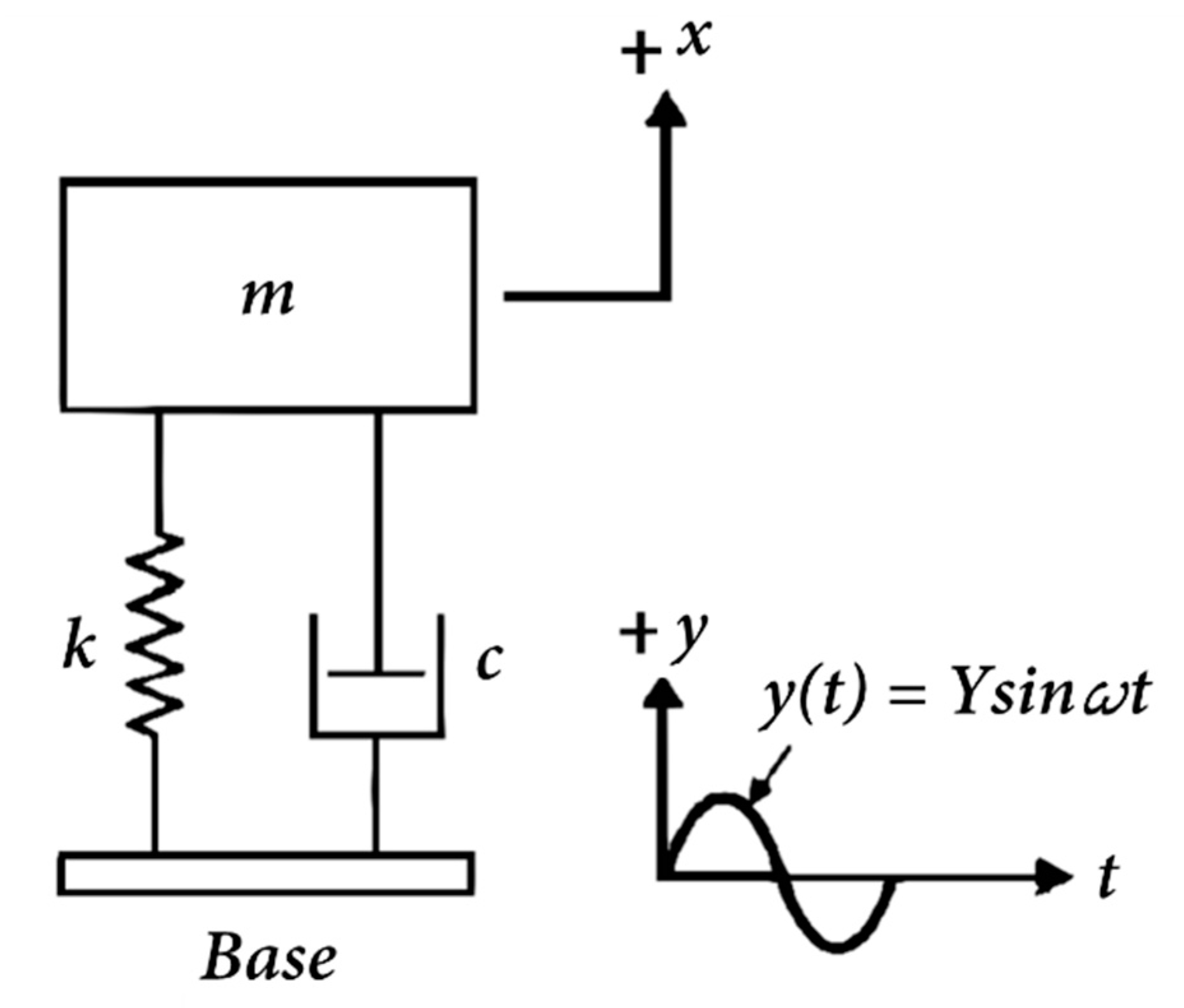
The one-DOF model is shown in
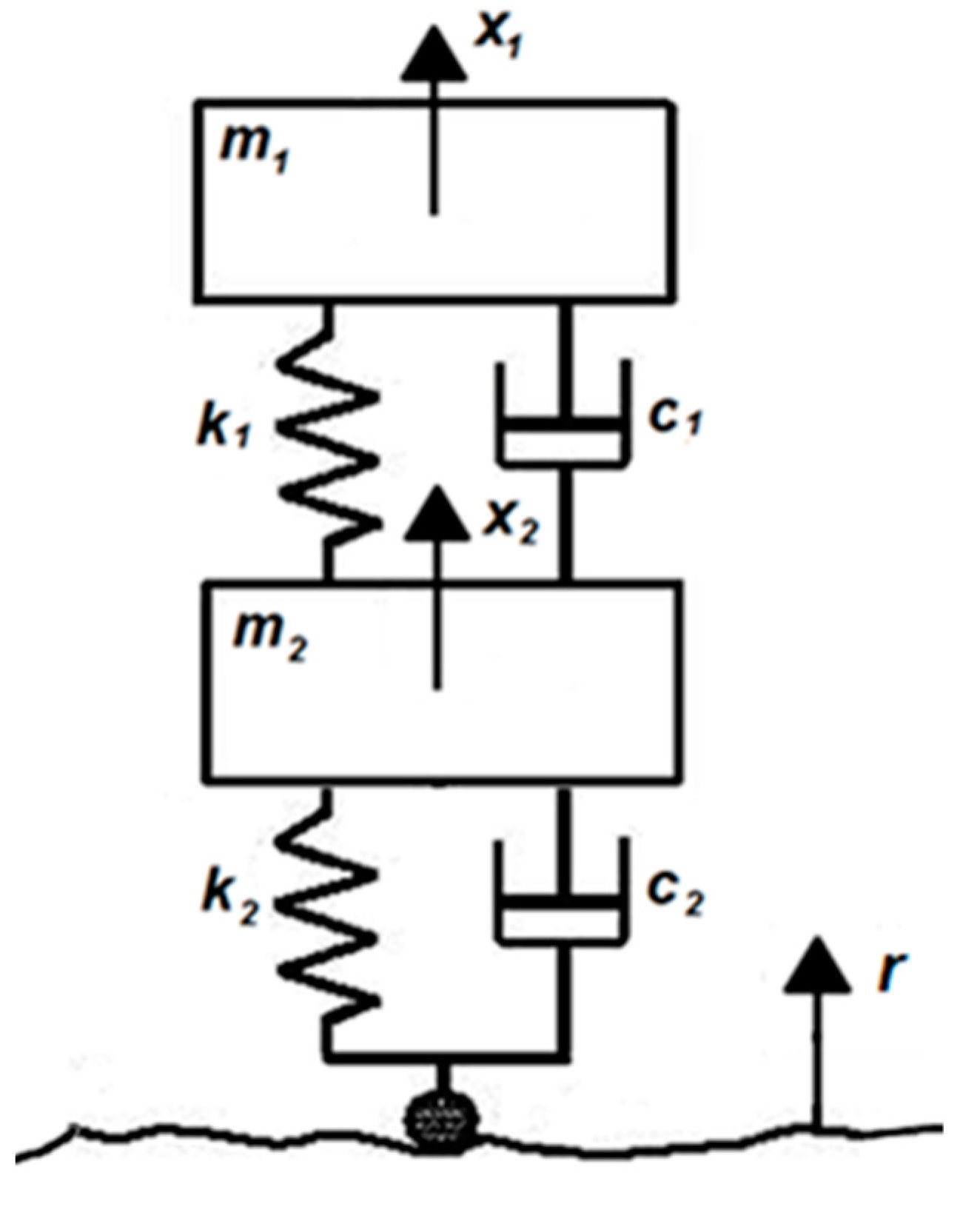
Figure 1 and its corresponding governing equation is given as Equation (1). The two-DOF model is shown in
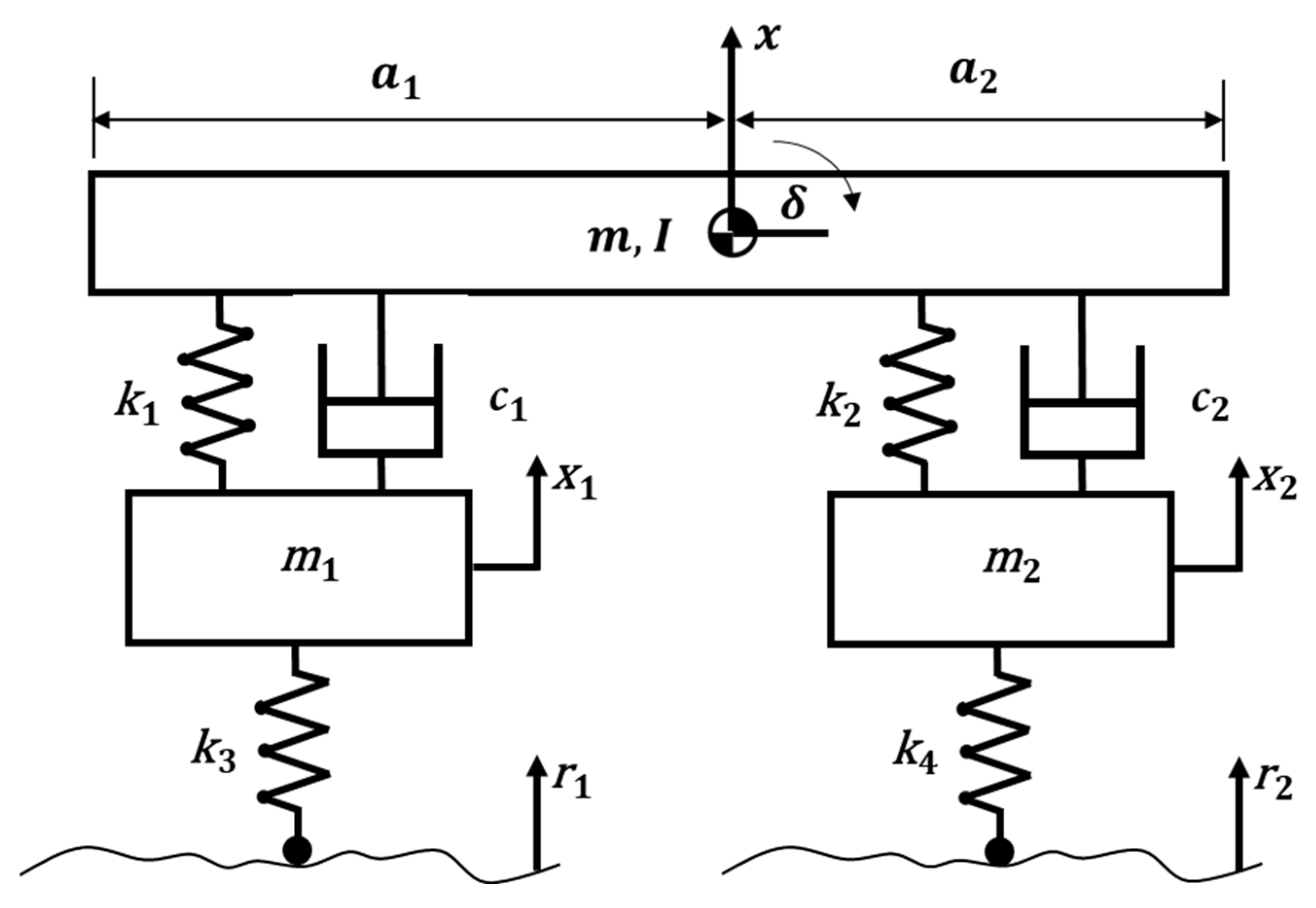
Figure 2 and its corresponding governing equations are given as Equations (2) and (3). Lastly, the bicycle model is shown in
Figure 3 and its governing equations are shown in Equations (4)–(7).
Then, we present the optimization and parameter identification tool (Figures 4–6), with an example of a two-DOF model, when the vehicle starts from a position of equilibrium (Figures 7 and 8), when passing over a curb (Figures 9–11), and when passing over a speed bump (Figures 12–14). The purpose of these examples is to ascertain if the tool has been correctly implemented by comparing these results with the expected behavior.
Afterward, we analyze our methodology with a set of experiments drawn from the Design of Experiments theory, in particular the Taguchi designs, whose use here is to provide a map of repeatability for all the experiments carried out. At this moment we concentrate on the one-DOF and two-DOF models. We understand here that we are facing an inverse problem with non-unique solutions, and we find that by restricting the space solution adequately we can find the exact suspension parameters in all cases.
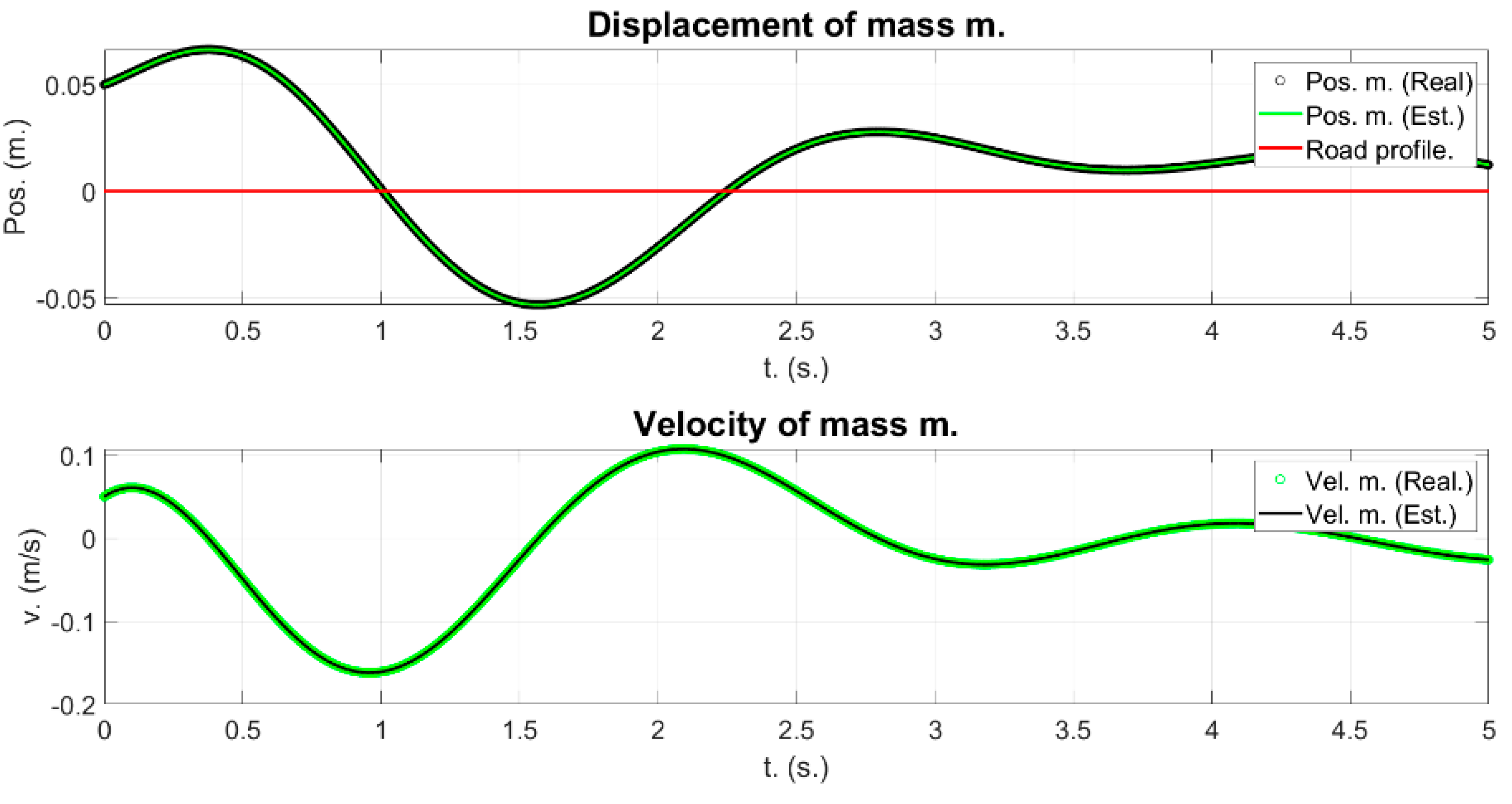
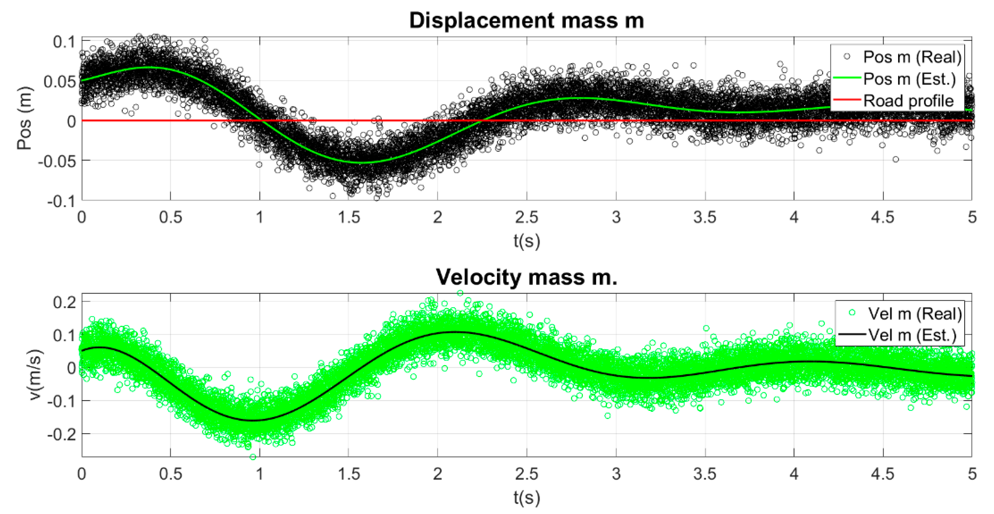
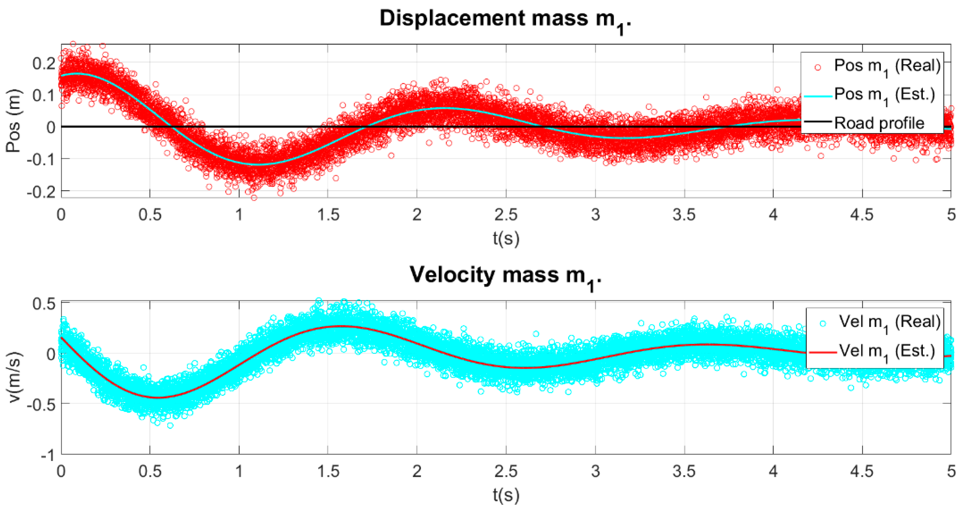
Finally, we extend our methodology to the bicycle model (4-DOF), where it is shown that it is possible to retrieve the exact suspension parameters, but the initial parameter from which the NM algorithm starts must be modified in some cases. Also, for the bicycle model, we present the use of this optimization process for the denoising of measurements.
4. Optimization and Parameter Identification Tool
With the tool developed in MatLab, the vertical behavior of a quarter-vehicle may be simulated, knowing the displacements and velocities of the masses for different excitation conditions: initial parameters, a curb, or a speed bump. In addition, it also allows for the importing of empirical data proceeding from real measurements.
After the last upgrade, the tool was able to simulate the vertical behavior as well as the pitching of the half-vehicle suspension, knowing the displacements, velocities, and accelerations of the masses for different excitation conditions: initial conditions outside equilibrium, after passing through a curb or a speed bump.
This simulation is carried out by providing the ode45 ordinary differential equations Solver from MatLab function with the set of differential equations that describe the dynamics of the system, which were discussed before. As they are a set of second-order differential equations, they must be provided as a set of first-order ones to be treated by the solver. Thus, for each coordinate of the masses (which also includes the angular dimension δ in the case of the bicycle model), we will also obtain its first derivative.
The most outstanding feature of this tool, besides simulation, is the parameter identification. Through this process, it is possible to obtain the characteristic parameters of the suspension system, unknown a priori, via an automatic finite number of iterations. It is enough to know the displacements or accelerations of the masses after sensorizing the movements of the vehicle suspension. An optimization process lies at the core of this feature.
This tool has the following behavior and requires the following entries:
- (1)
Target parameters that allow for the vertical movement simulation of the quarter- or half-vehicle (Procedure 1 or theoretical) or data coming from the sensorization of the vehicle (Procedure 2 or practical);
- (2)
User-defined initial parameters from which the identification process will take place.
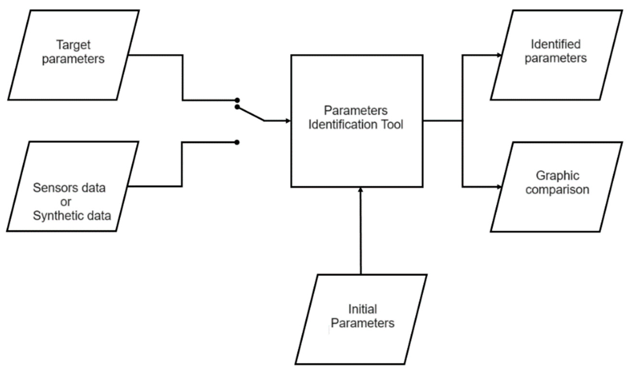
As outputs of this process, the identified parameters are obtained as well as a graphic comparison between the initial curve and the identified one.
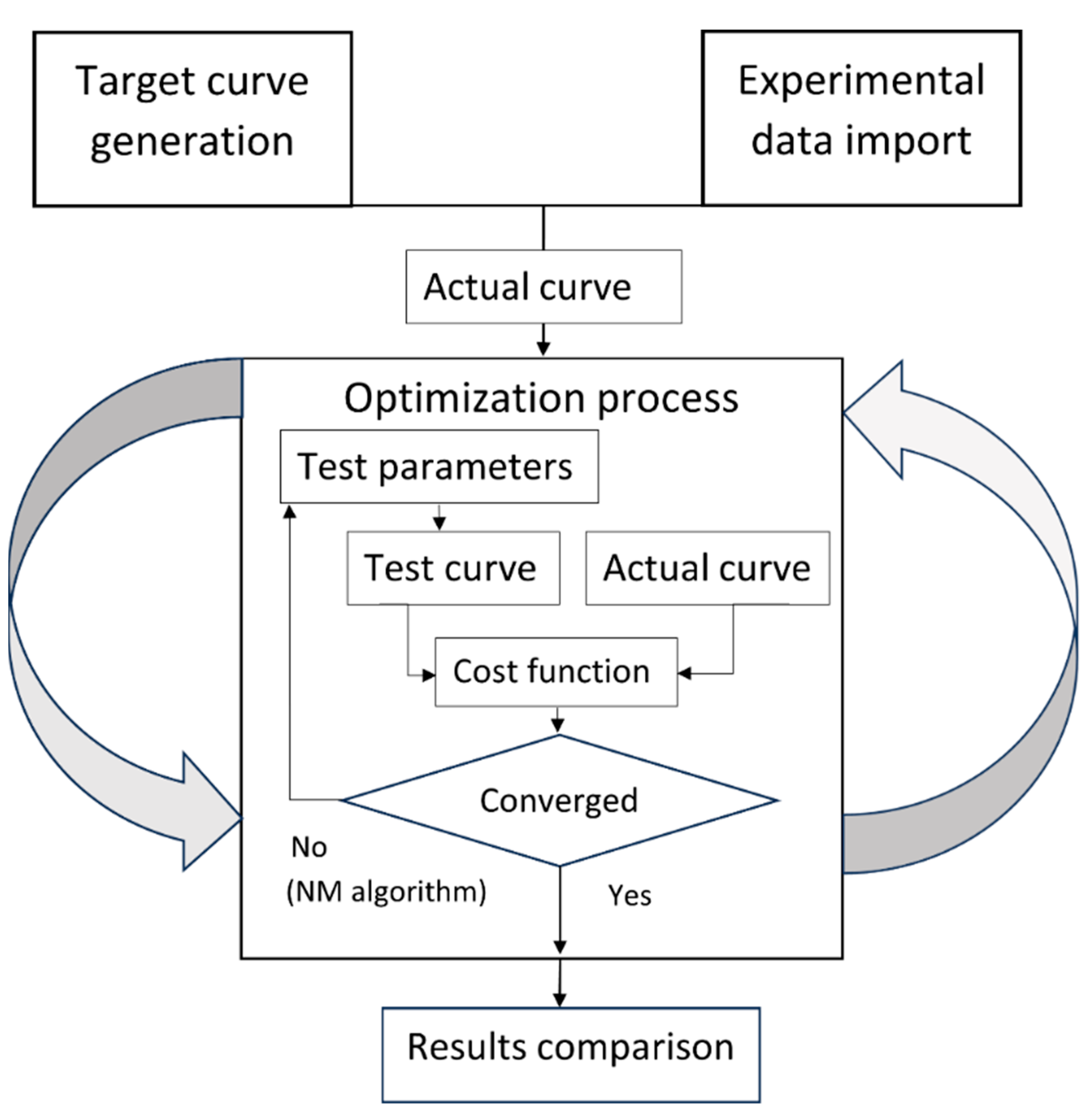
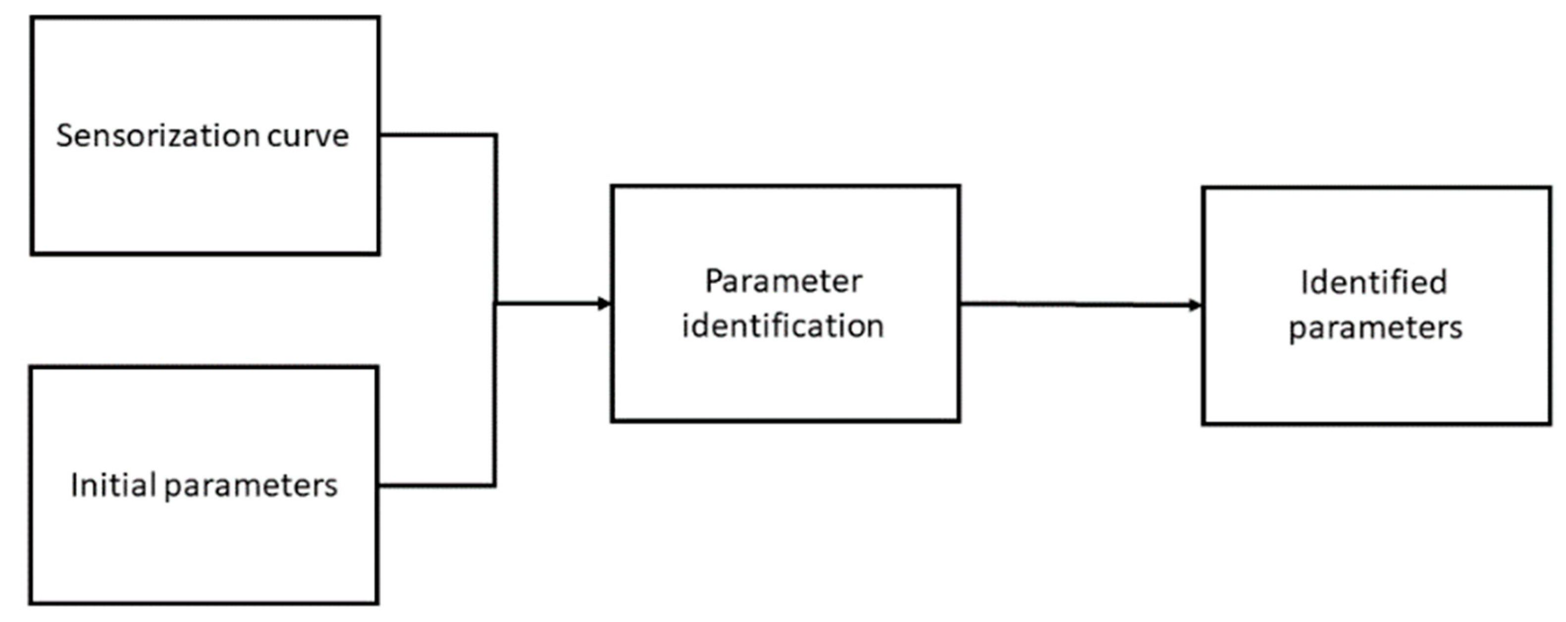
The place of the parameter identification tool in the methodology proposed is described in
Figure 4.
Figure 4.
General functional schema of the methodology for parameter identification.
Figure 4.
General functional schema of the methodology for parameter identification.
Whatever the procedure, the optimization process undergoes three main phases, detailed in
Figure 5:
Figure 5.
Main phases (parameter identification tool).
Figure 5.
Main phases (parameter identification tool).
Therefore, the process is the following:
Whether from a simulated target curve or from an experimental one, we obtain an actual curve. We provide a set of initial parameters, which, from the corresponding model, a test curve will be obtained. By providing a cost function—and in this work two cost functions are considered—the actual and the test curves can then be compared. If we reach convergence, the process stops, and we obtain a set of parameters that we compare with the actual ones. If we do not reach convergence, the Nelder–Mead algorithm selects a new set of parameters, which in turn generates a test curve to be compared with the actual curve via the cost function of our choice; this process is repeated until convergence.
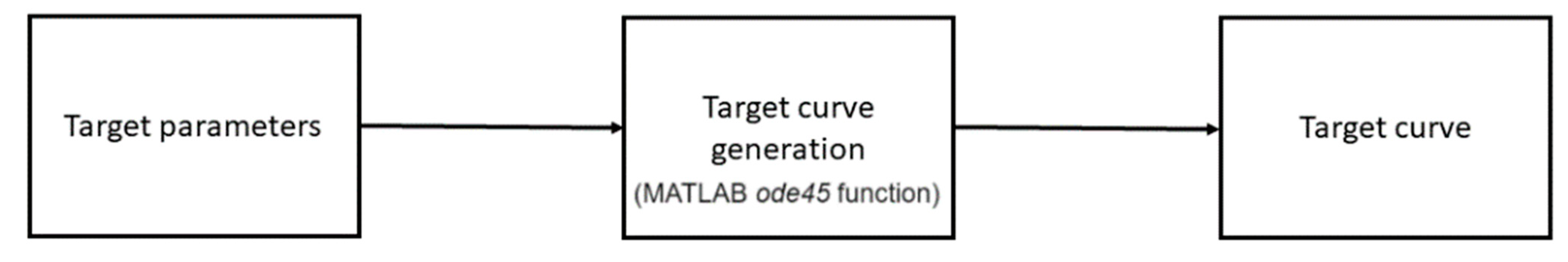
4.1. Generation of the Target Curve
We can obtain the “target curve” via two different methods. The first of them is by importing empirical data coming from the sensorization of the suspension of a vehicle, or by defining the following parameters, which, in the example we show here for a quarter-vehicle model are (
Table 1):
These data apply to the schema shown in
Figure 2. These values were drawn from work by Sharma and Saluja [
35].
Moreover, the way the system is excited must be chosen. In this case (
Table 2):
Thus, the schema for the generation of the target curve is as described in
Figure 6:
Figure 6.
Schema of the generation of the target curve.
Figure 6.
Schema of the generation of the target curve.
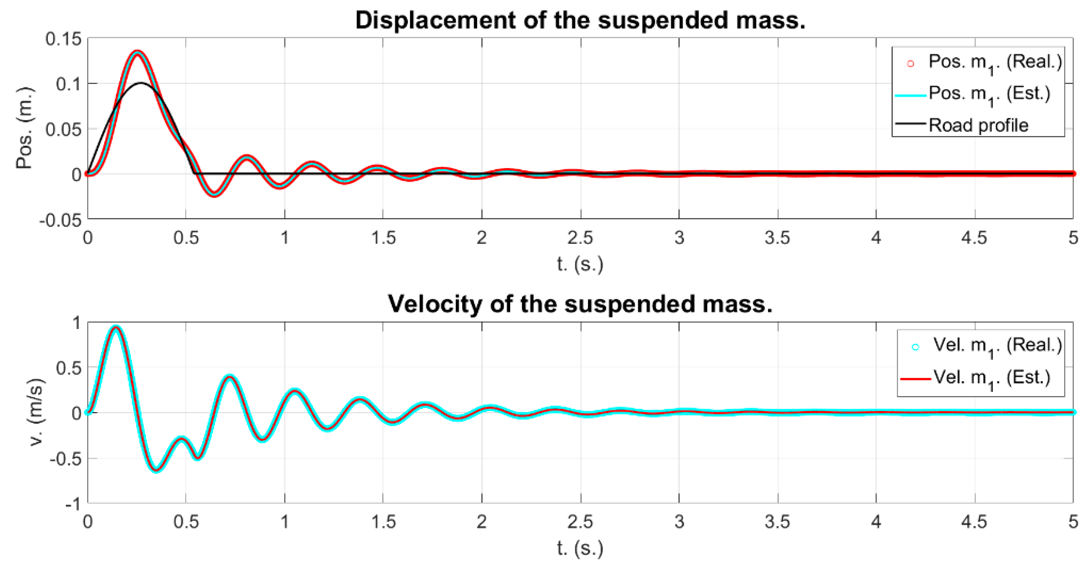
By setting the target parameters and the initial values—and a possible road profile that must be set programmatically in the model—the target curve via the ode45 MatLab function can be generated. In the case of a two-DOF model, we must set the suspended mass m1, the suspension spring rigidity k1, the suspension damping coefficient c1, the unsprung mass m2, the tire rigidity k2, and the tire damping coefficient c2. Also, the initial positions and velocities of the suspended—x01 and v01—and unsprung masses—x02 and v02—must be set.
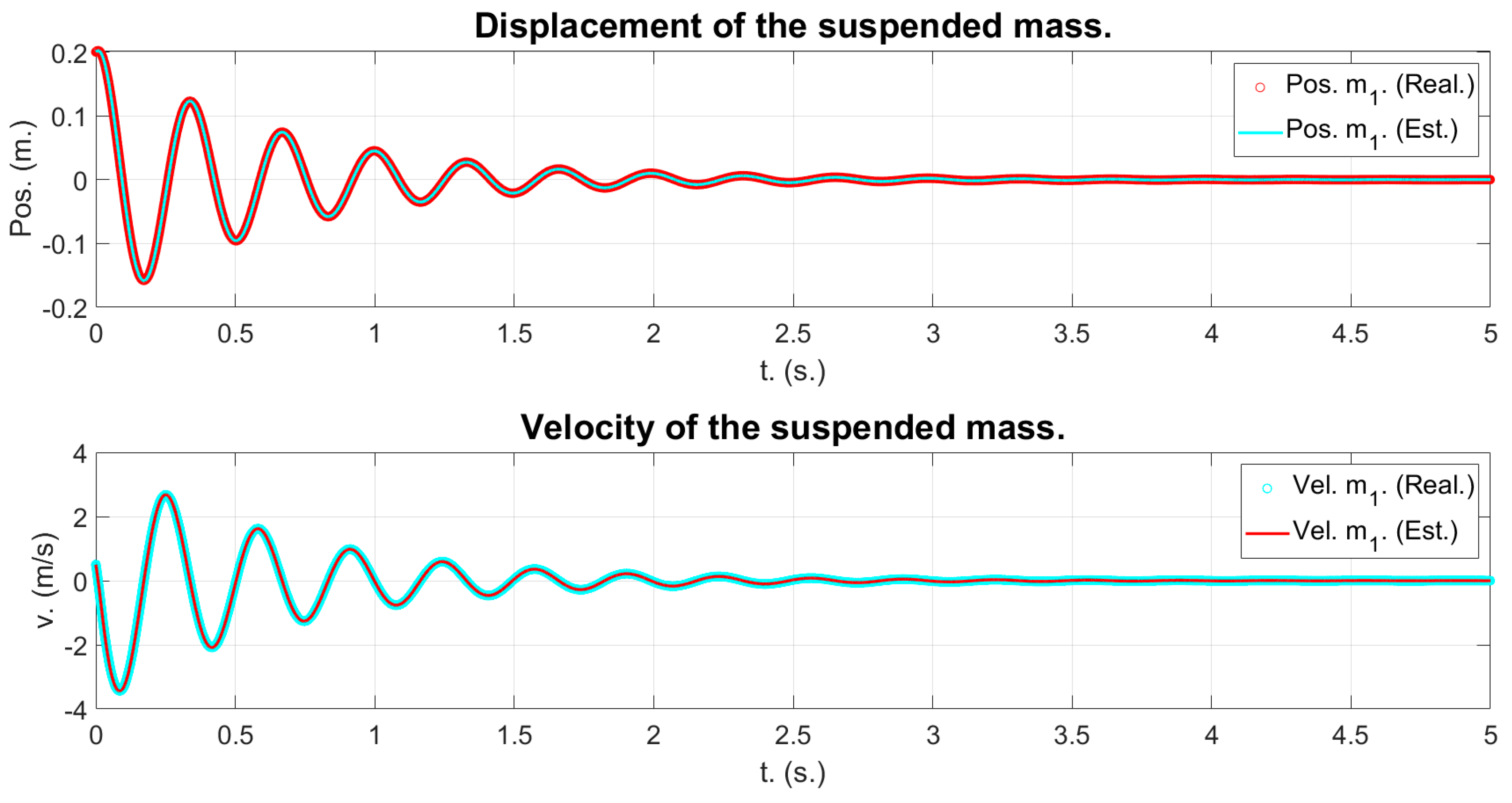
Figure 7.
Displacement and velocity of the suspended mass.
Figure 7.
Displacement and velocity of the suspended mass.
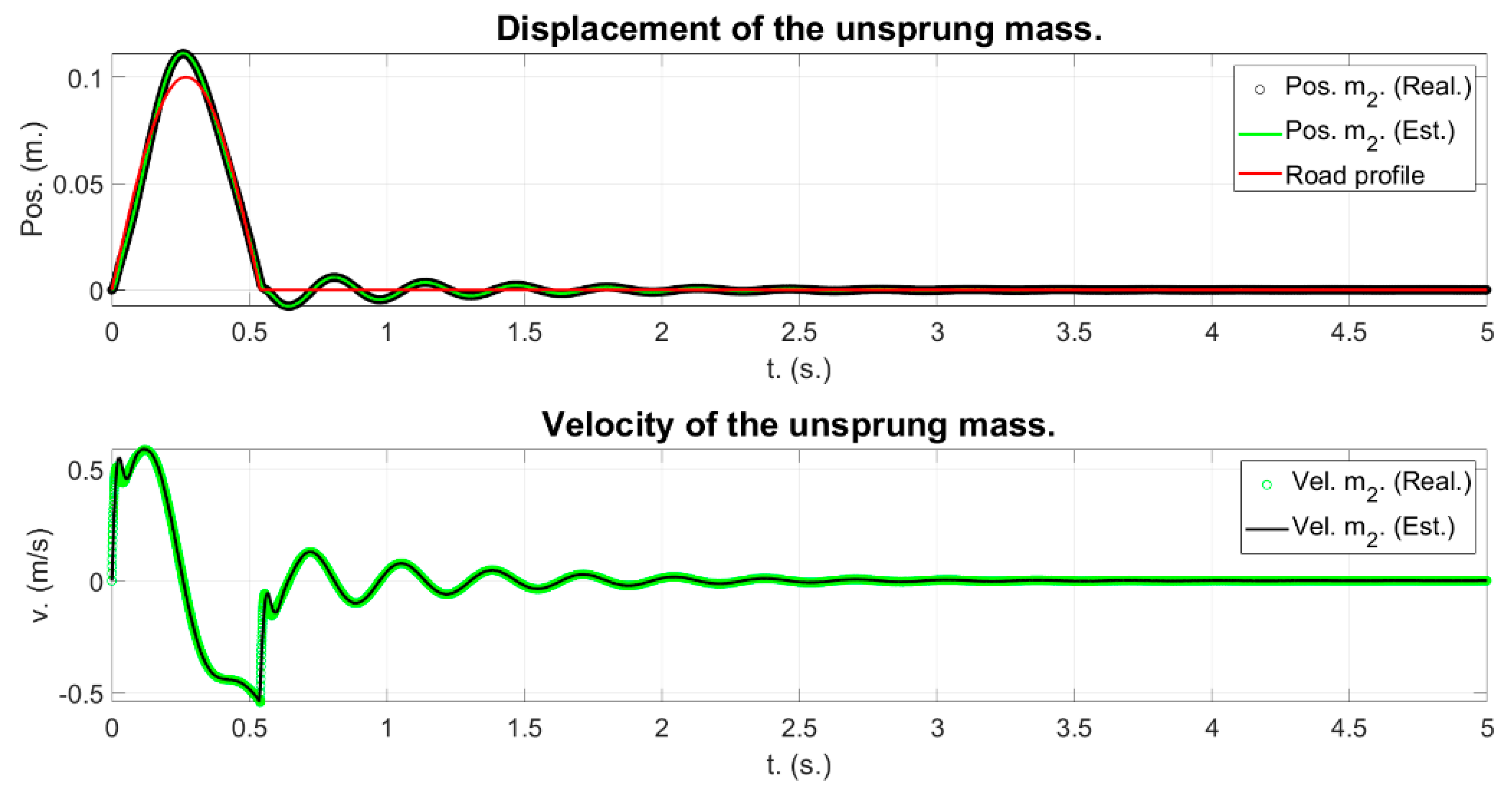
Figure 8.
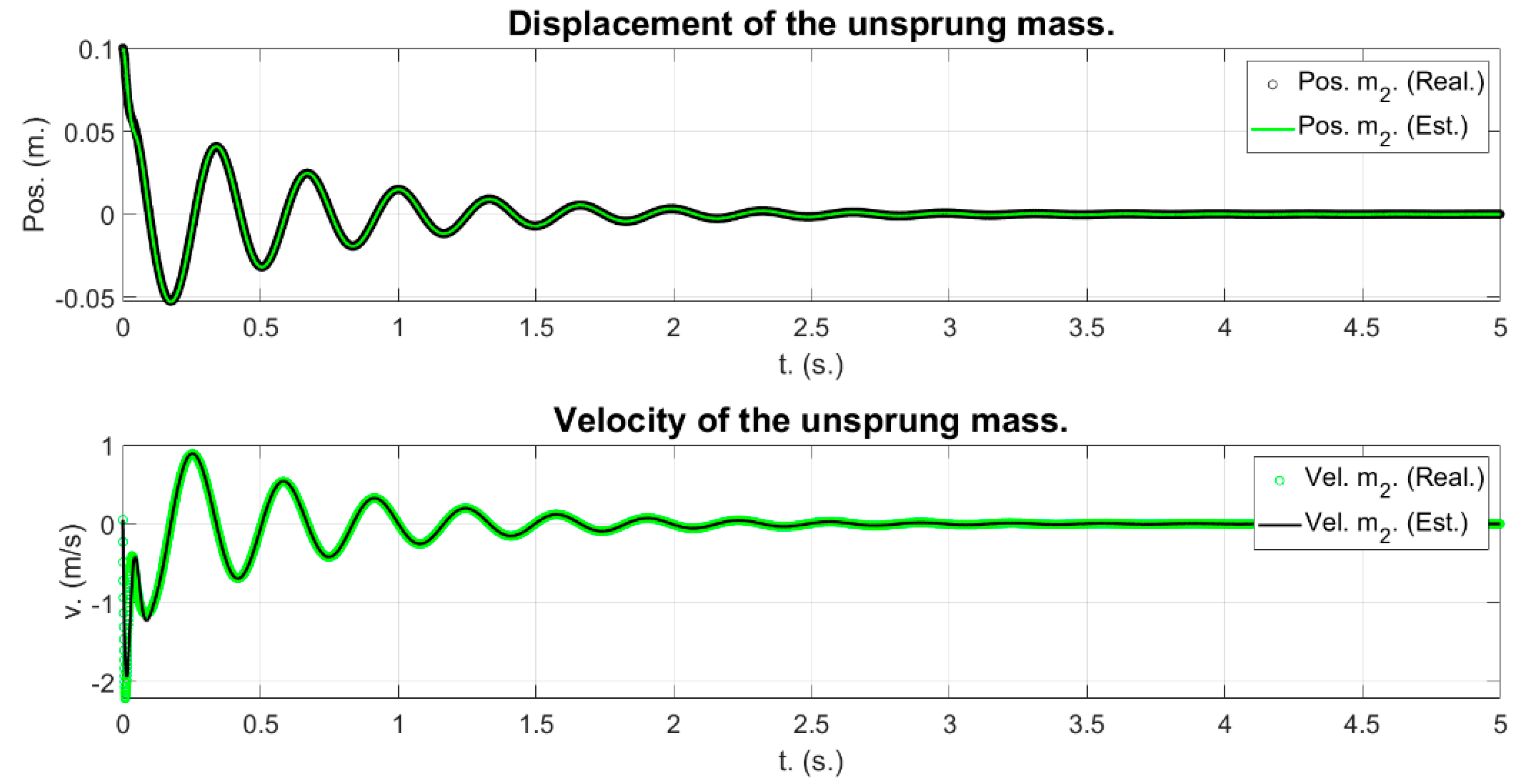
Displacement and velocity of the unsprung mass.
Figure 8.
Displacement and velocity of the unsprung mass.
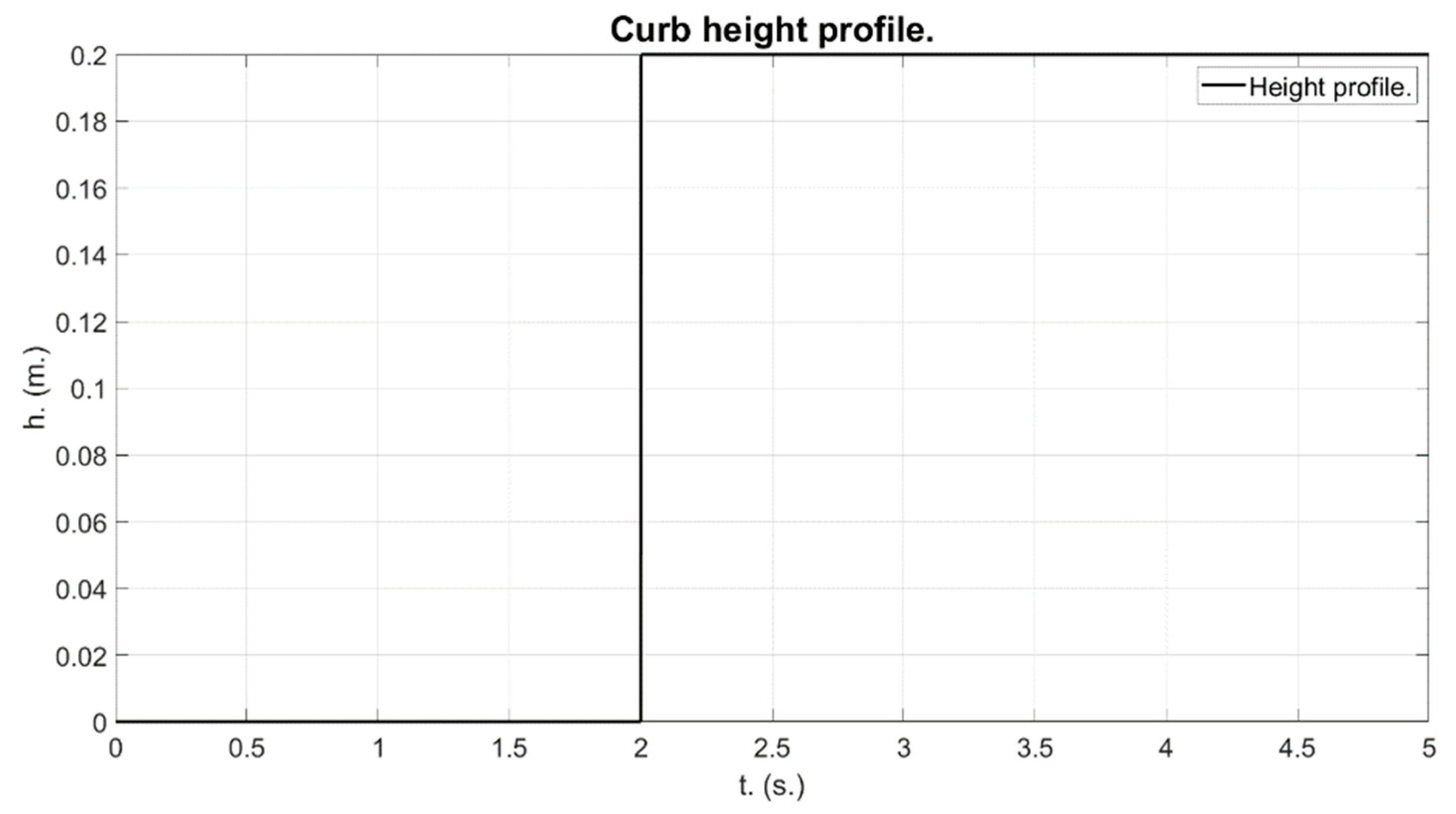
Going over a curb is shown in
Figure 9. The curb’s height must be defined (h). The results may be found in
Figure 10 and
Figure 11, and they show an accord with the expected behavior:
Figure 9.
Curb profile used for simulation as input function for system response.
Figure 9.
Curb profile used for simulation as input function for system response.
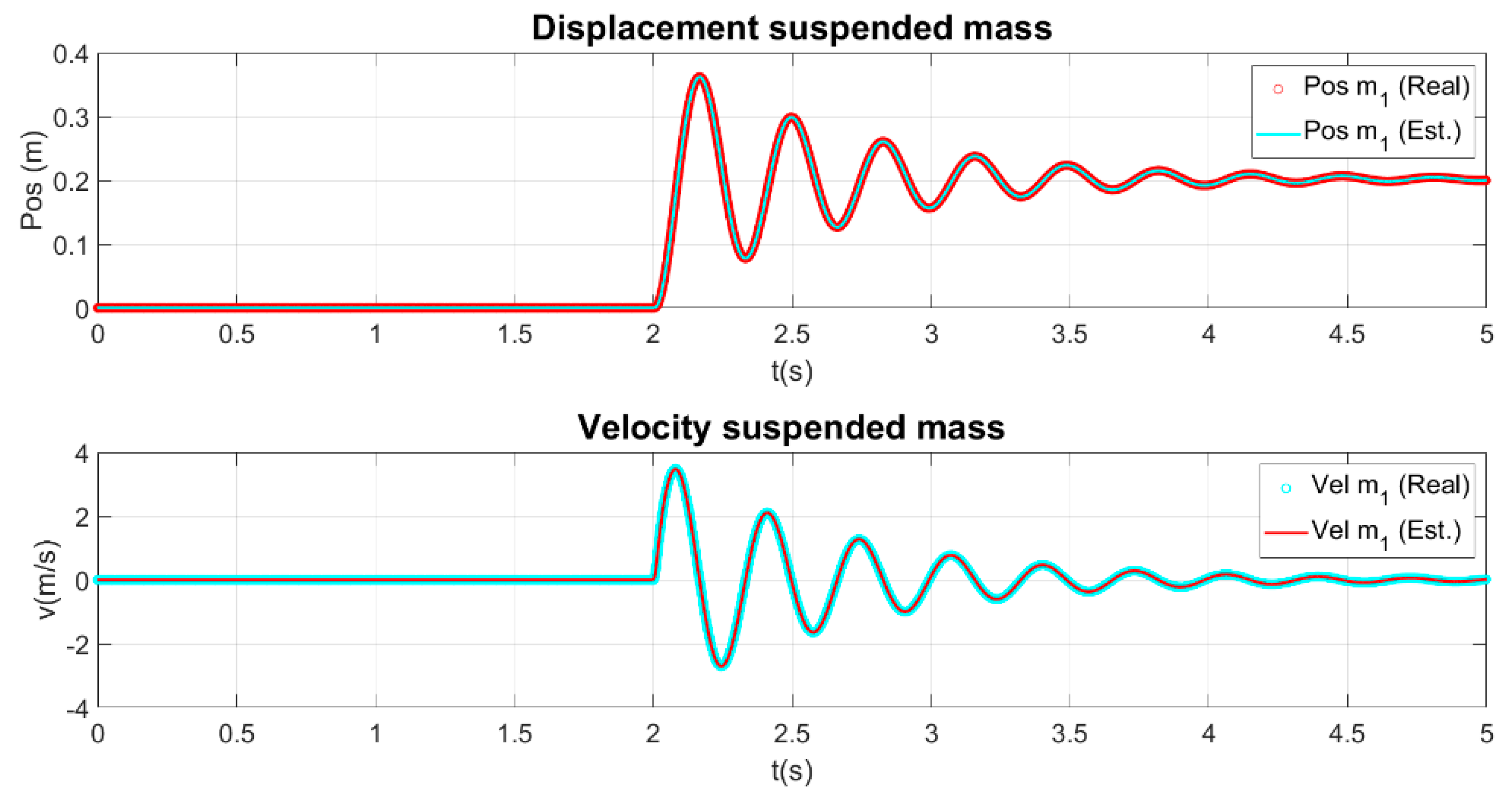
Figure 10.
Displacement and velocity of the suspended mass for a step input.
Figure 10.
Displacement and velocity of the suspended mass for a step input.
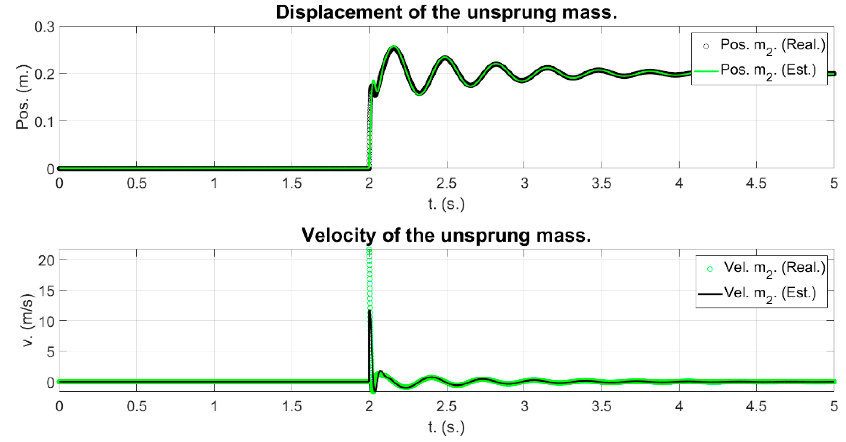
Figure 11.
Displacement and velocity of the unsprung mass for a step input.
Figure 11.
Displacement and velocity of the unsprung mass for a step input.
Here, both initial positions and velocities are set to zero.
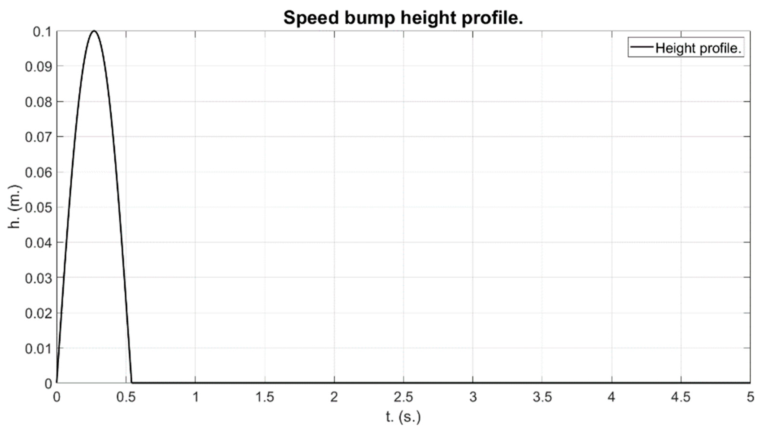
Going over a speed bump is shown in
Figure 12. The speed bump’s height can be configured (h = 0.1 m), its length (l = 3 m), and the velocity the vehicle crosses it with (v = 20 km/h). The results can be found in
Figure 13 and
Figure 14:
Figure 12.
Speed stop profile used as input functions for system response.
Figure 12.
Speed stop profile used as input functions for system response.
Figure 13.
Displacement and velocity of the suspended mass after passing over a speed bump (black).
Figure 13.
Displacement and velocity of the suspended mass after passing over a speed bump (black).
Figure 14.
Displacement and velocity of the unsprung mass after going over a speed bump (red).
Figure 14.
Displacement and velocity of the unsprung mass after going over a speed bump (red).
Here, the initial positions and velocities are set to zero too.
4.2. Parameter Identification
The addition and innovation of this research is that it allows us to go in the opposite direction. That is, based on the curves of the movement of the masses obtained via sensorization of the vehicle suspension, the tool allows for the computation of the suspension parameters, as shown in
Figure 15.
In this case, the input consists of the sensorization of the vehicle suspension that allows for knowledge of the displacements or accelerations of the masses as a function of time. Besides the empirical curve, this phase needs another input, namely the initial parameters. These are the values from which the iterative process starts until it can identify the unknown parameters.
In this phase, the identification parameter program is executed, using the
fminsearch included in the MatLab library that has as its aim at finding the minimum of a scalar function of several variables, starting from an initial guess (initial parameters), using the Nelder–Mead algorithm. This is known as unrestricted non-lineal optimization. This function implements the simplex Nelder–Mead algorithm by Lagarias et al., as described in [
36].
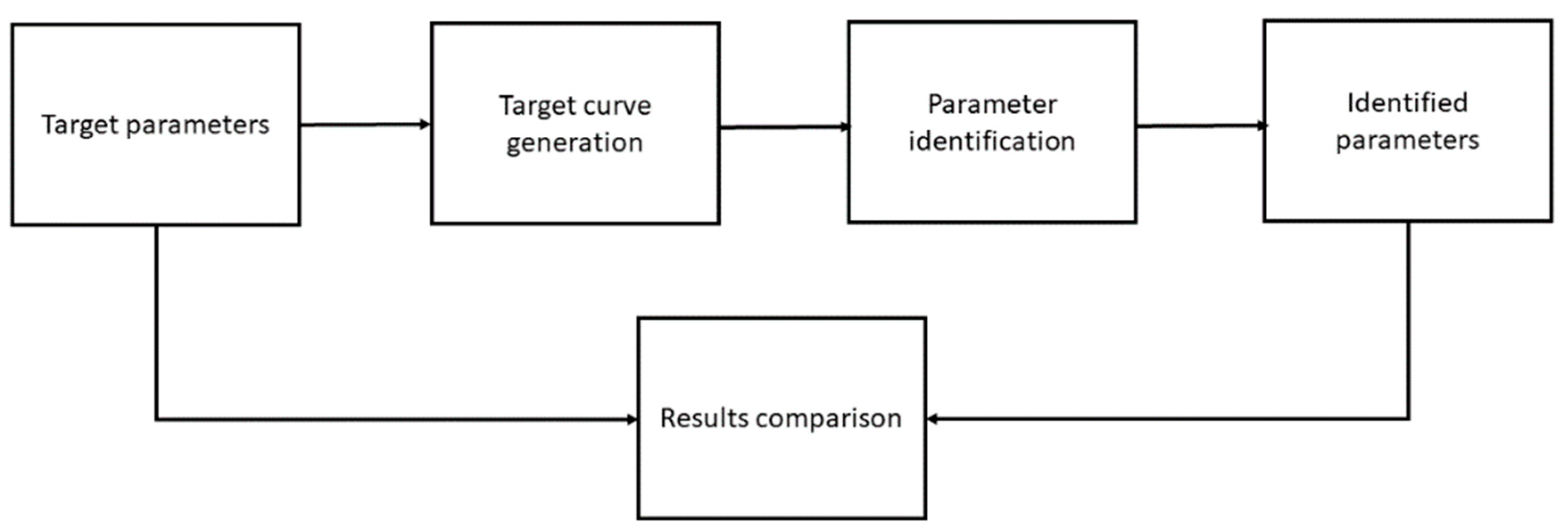
4.3. Results Comparison
Finally, a comparison between the target parameters and the identified parameters is made. This allows for the assessment of the quality of the identification (
Figure 16).
One of the outputs of the fmisearch is the set of identified parameters. This set of parameters can be readily compared numerically with the target parameters. This comparison can be made as an absolute value and/or as a percentual value. The percentual error value was found to be homogeneous across the set of identified parameters. Successful parameter identification means that the error was zero or negligibly small.
5. Experimental Recovery of Suspension Parameters with Nelder–Mead Optimization
To evaluate the effectiveness of the indicated optimization methodology in relation to the sensitivity of parameters to be identified within the dynamic equations of motion, a parameter analysis process is employed through the Design of Experiments (DoE). Among the various analytical possibilities within DoE, we selected the Taguchi method for our study for several reasons. Firstly, the Taguchi method is renowned for its efficiency in examining a large number of variables with a relatively small number of experiments, which is crucial in complex dynamic systems like vehicle suspensions (and even more important when experimental runs need to be reduced to reduce the overall cost). This efficiency stems from its orthogonal arrays, which ensure that all parameters are independently evaluated, providing clear insight into their individual effects and interactions.
Secondly, the Taguchi method focuses not just on the mean performance characteristics but also on the variability, which is essential when dealing with dynamic systems where parameters may be sensitive and prone to fluctuation. This approach enables us to understand not only which parameters are most influential, but also how robust the system’s performance is in response to variations in these parameters.
Lastly, the method’s concept of the signal-to-noise (S/N) ratio is particularly useful in this context. It helps in optimizing performance characteristics against the noise of the system—in this case, the inherent uncertainties in dynamic suspension parameters. By using the Taguchi method, we aim to identify the optimal set of parameters that not only achieve the desired suspension dynamics but also ensure robust performance against variations and uncertainties in the system.
As stated before, the
fminsearch function is used for parameter identification. This function uses the Nelder–Mead algorithm. At this point, it is pertinent to ask the question of how accurate the set of identified parameters is. To analyze this, a battery of tests based on the Taguchi theory was carried out, specifically the 16 factors with four levels for each design (L16-4 design) for the one-DOF model and the 13 factors with three levels for each design (L27-3 design) for the two-DOF model. The order of experiments was obtained via the R qualityTools package (version 1.55) [
37] with no randomization for ease of replication. Also, for both cases, the starting point for the variables subject to optimization was set to half the true ones except for the mass, which is supposed to be known and was set initially to its true value.
This means that, in the case of the one-DOF model, for each of the initial conditions and suspension parameters x
0, v
0, m, c, k, labelled A, B, C, D, and E, sixteen experiments varying their values according to four levels (values) were carried out. Different values for each of the levels can be found in
Table 3. The corresponding order of experiments with its values can be found in
Table 4.
In the case of the 2-DOF model, labels A through K stand for x
01, v
01, x
02, v
02,
m1,
c1,
k1, m2,
c2, and
k2. Labels L through N remain unused. Twenty-seven experiments were carried out, varying their values according to three levels (values). Different values for each of the levels can be found in
Table 5 whereas the corresponding order of experiments with its values can be found in
Table 6.
The fminsearch needs a cost function to be minimized, and two cost functions were considered, adapted to the dimensionality of the problem.
The first minimizes the sum of squares of the differences between the positions of each of the masses in the system under consideration, where the difference is meant to be obtained between the simulated, theoretical solution, and the Nelder–Mead tested (theoretical procedure) or the one obtained between the sensor curve and the Nelder–Mead tested (practical procedure).
The second is simply the Frobenius norm of the Ytheor-Ytest matrix in the case of the theoretical procedure and the Ysensor-Ytest in the case of the practical procedure. Ytheor is the matrix obtained via the simulation through the ode45 MatLab function, Ytest is the matrix obtained through this same function in the optimization iterative process, and Ysensor is the one obtained through the embarked sensorics.
5.1. One-Degree-of-Freedom Model
For all the tests detailed in
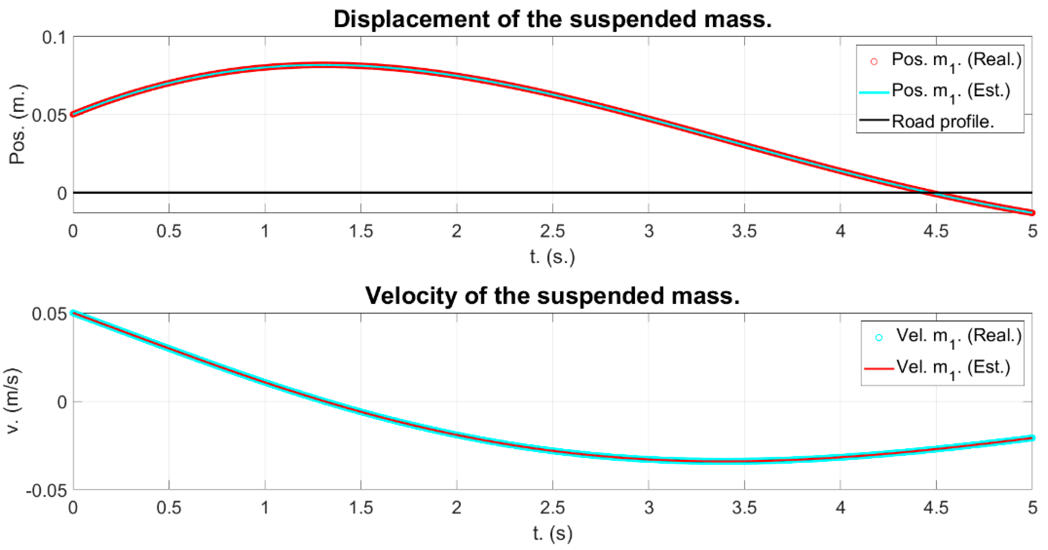
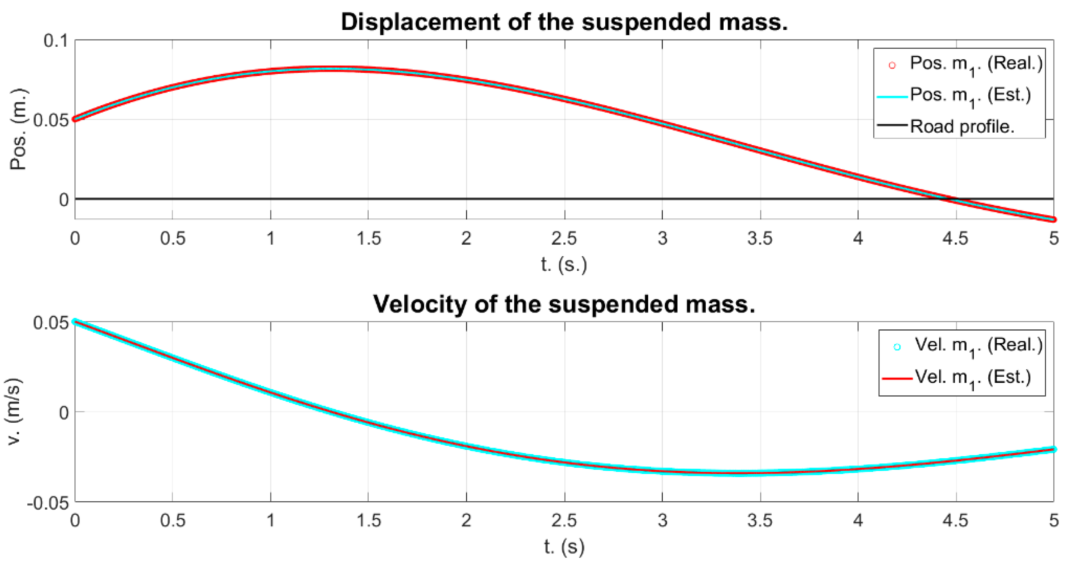
Table 4 and for both cost functions, if no restrictions were imposed, the obtained parameters presented errors of circa −40%. This could not be readily seen from the graphics because perfect reconstruction of the curves themselves was obtained in all the cases. This effect would also be seen in the remaining models under consideration. For the first and second cost functions we obtained (
Figure 17 and
Figure 18):
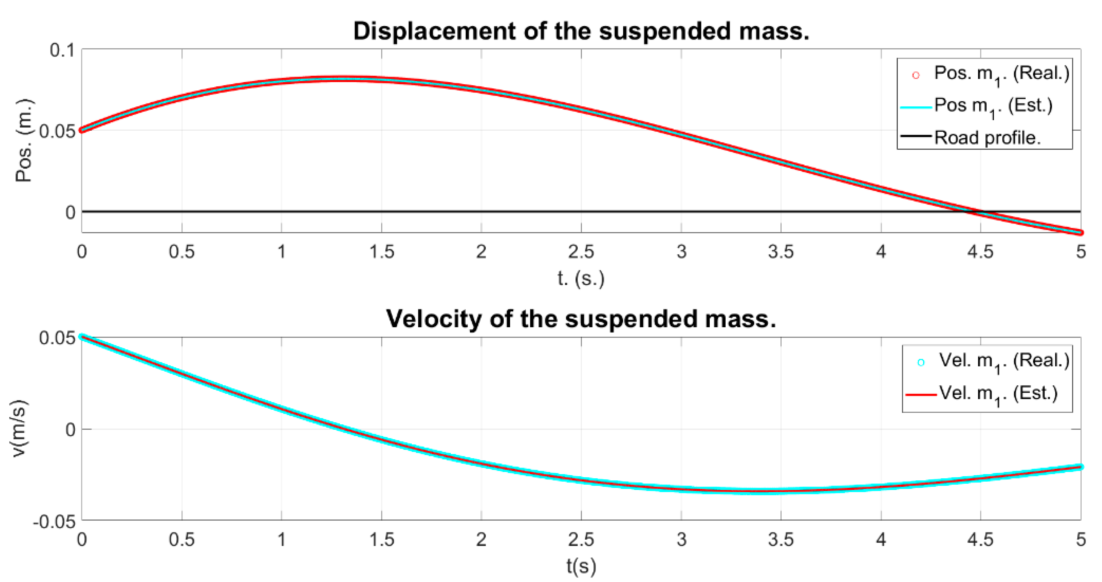
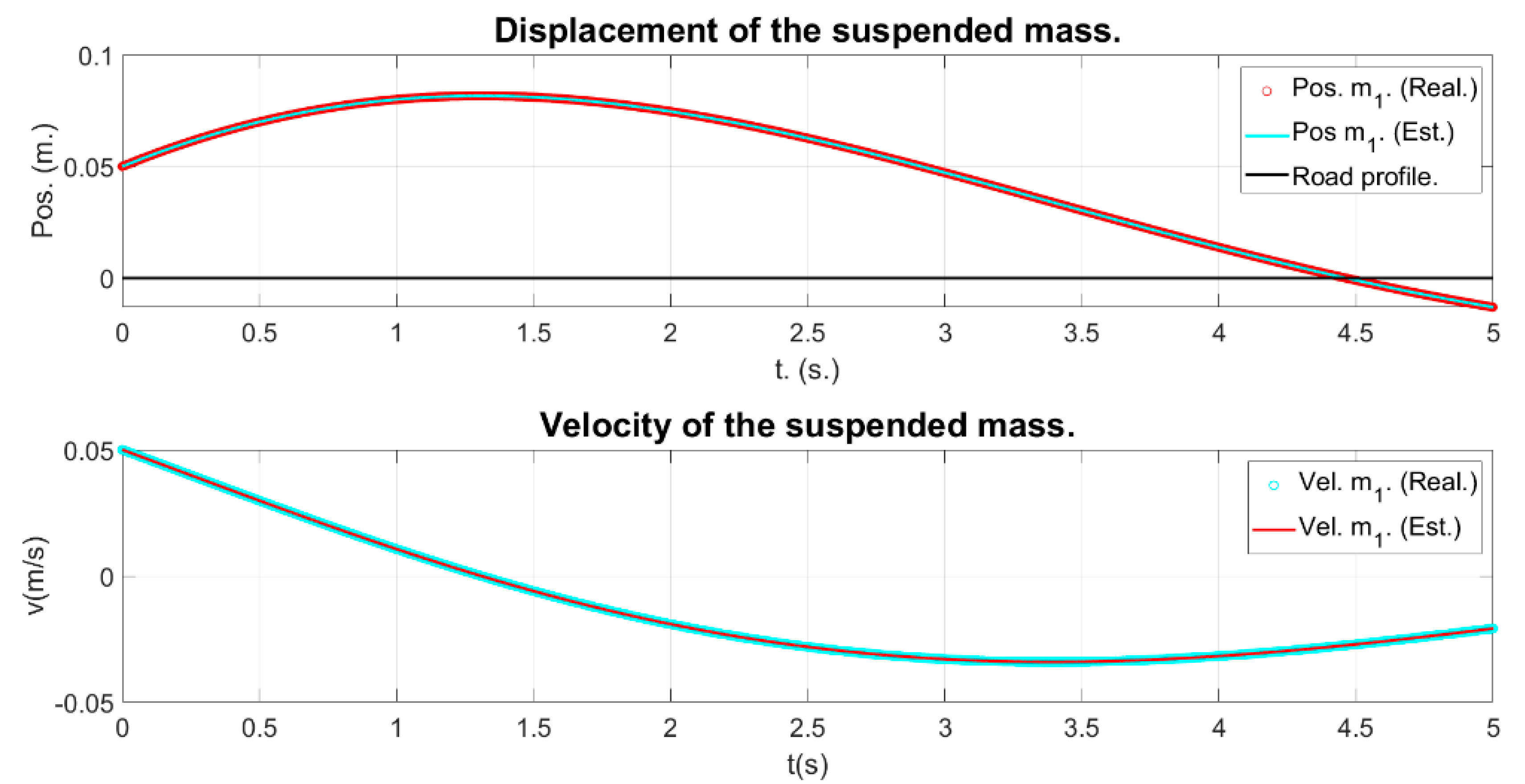
At this point, it is clear that this is an inverse problem with a non-unique solution. Therefore, the solution space had to be restricted. This can be carried out by setting a parameter to a fixed value, and the most obvious parameter is the mass, which can be readily measured and consequently was set to its true value. Then, for the first and second cost functions (
Figure 19 and
Figure 20):
This was performed programmatically via setting the mass as a global variable.
Here, it must be stressed that adequate parameter identification cannot be ascertained from the figures themselves—which are undistinguishable—and which are obtained from the unrestricted optimization schema (
Figure 17 and
Figure 18) and from the restricted optimization schema (
Figure 19 and
Figure 20). Likewise, by using different cost functions (
Figure 17 and
Figure 19 for the first cost function, and
Figure 18 and
Figure 20 for the second cost function), we cannot ascertain if successful parameter identification was obtained, as the target curve is perfectly recovered in all cases. Only the restricted optimization schema successfully recovers the correct suspension parameters.
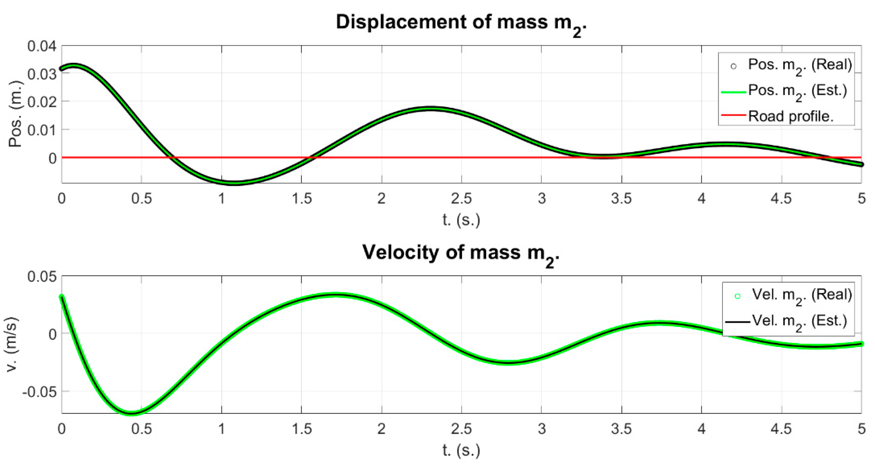
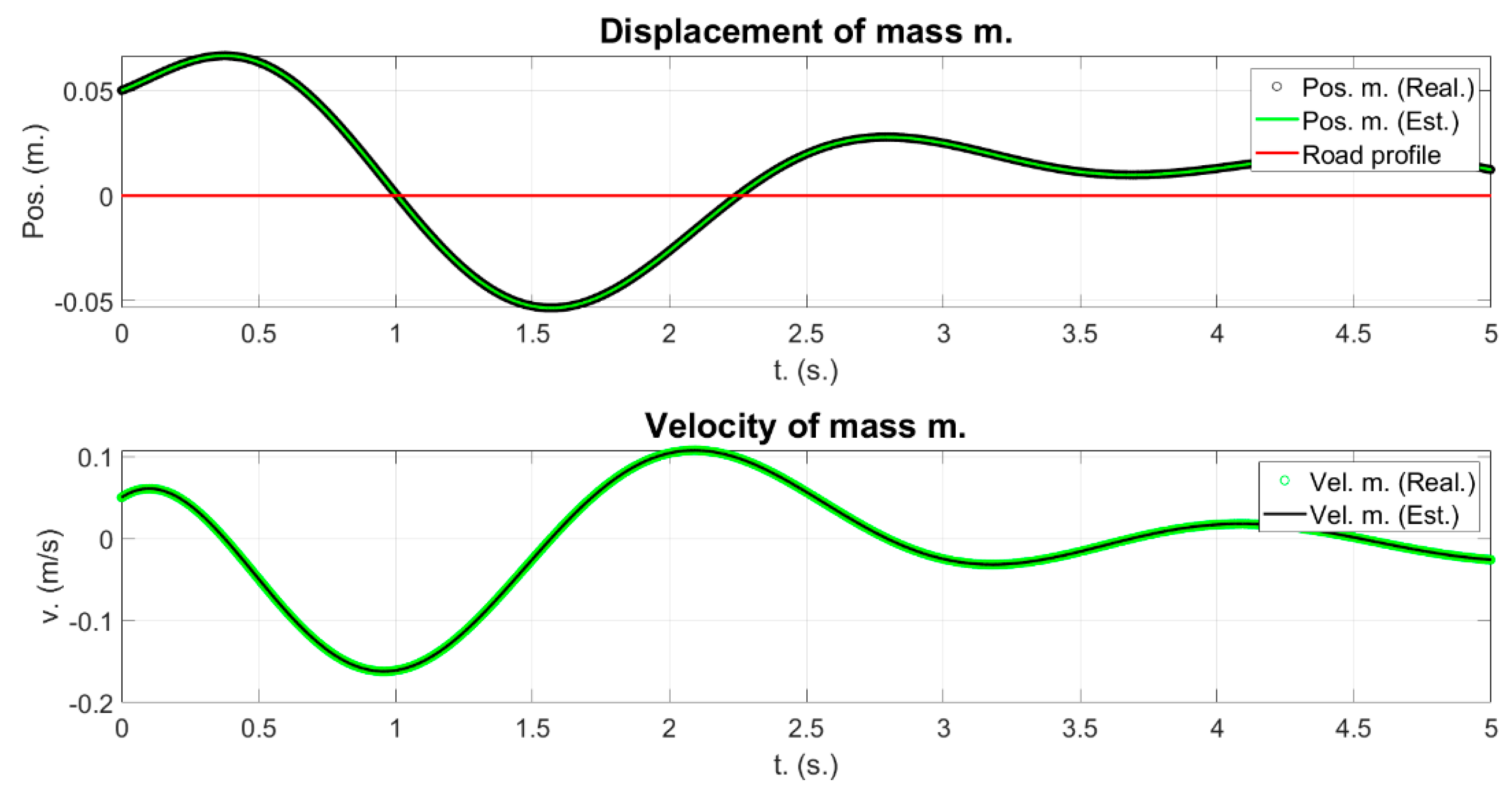
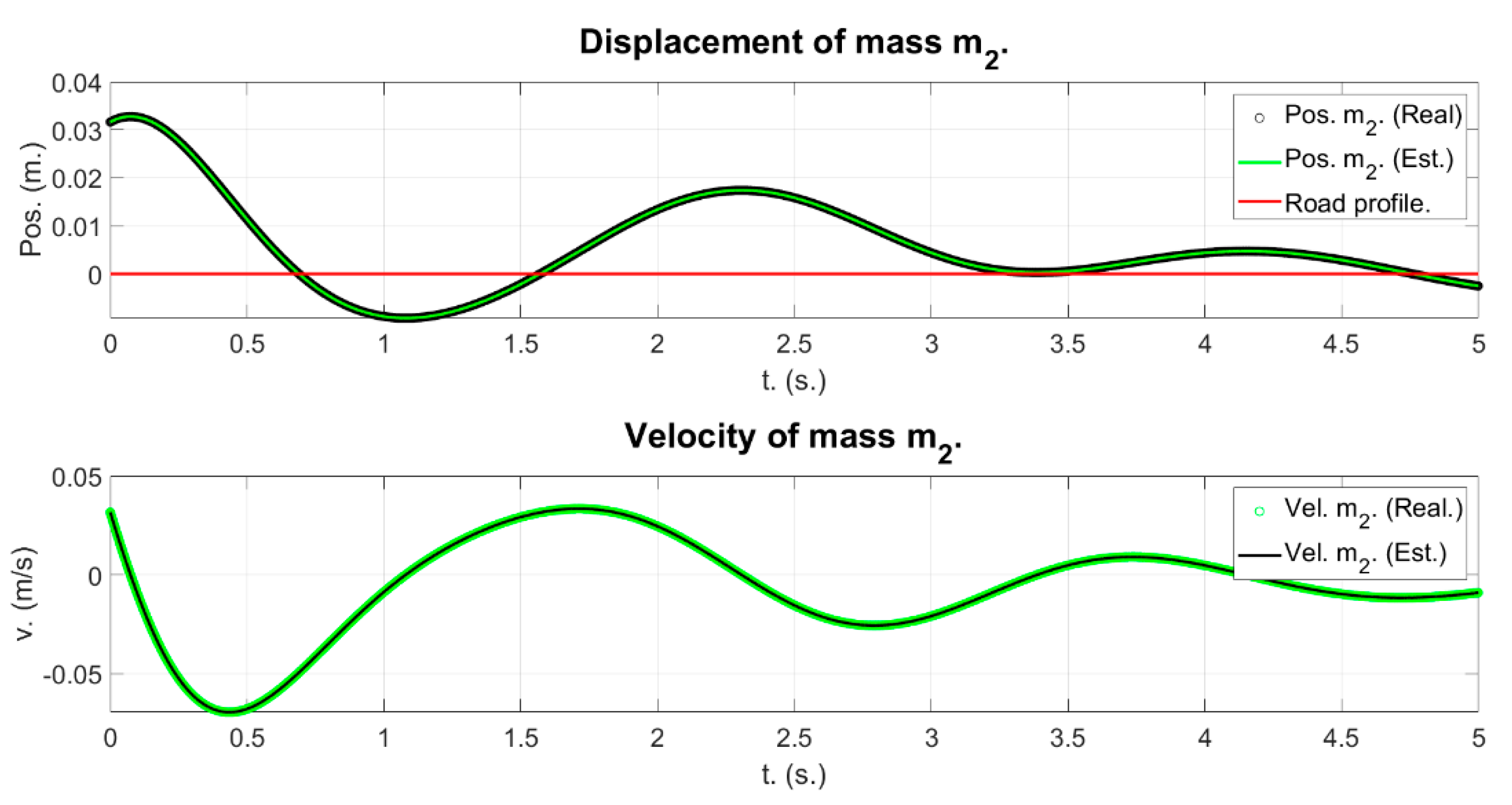
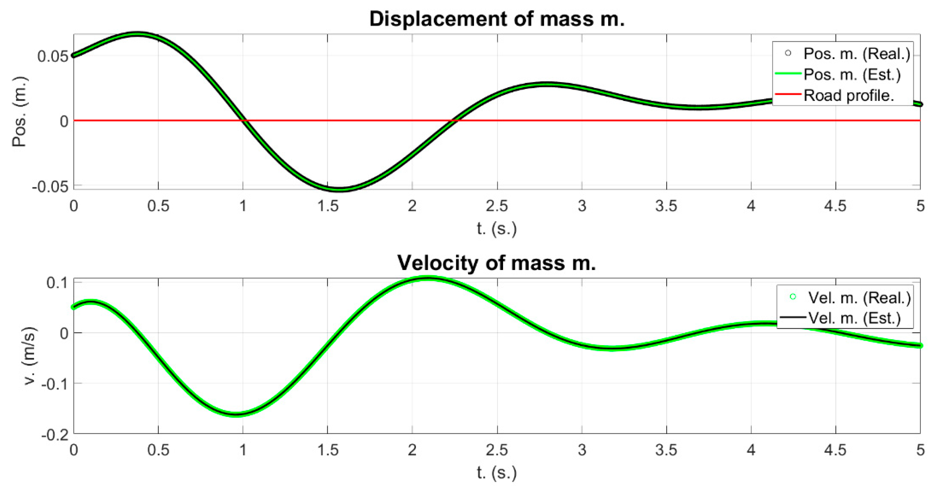
5.2. Two-Degrees-of-Freedom Model
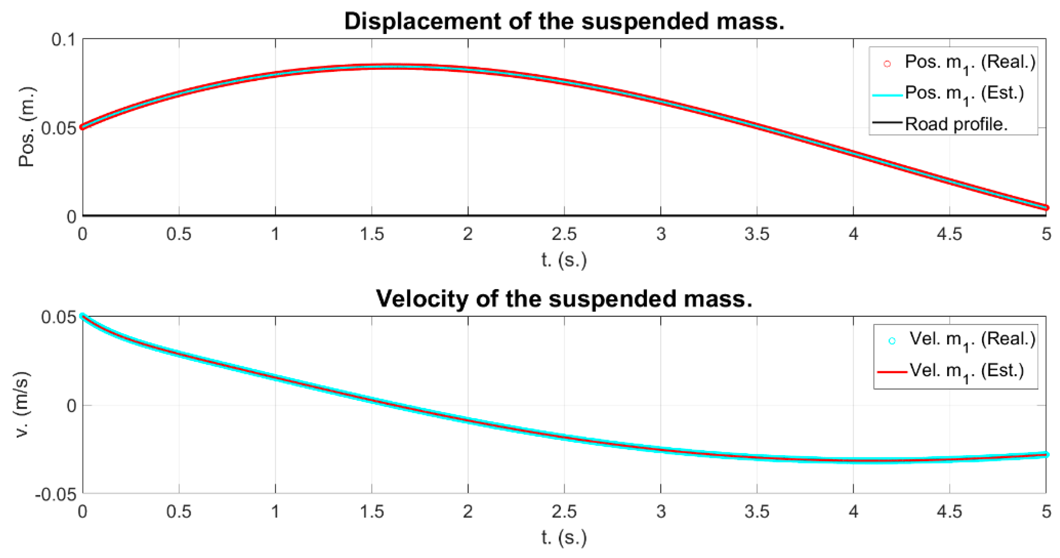
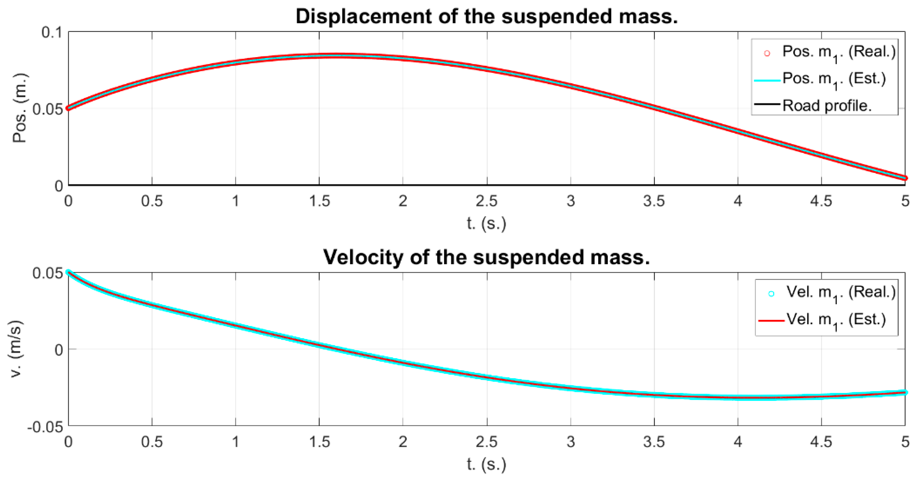
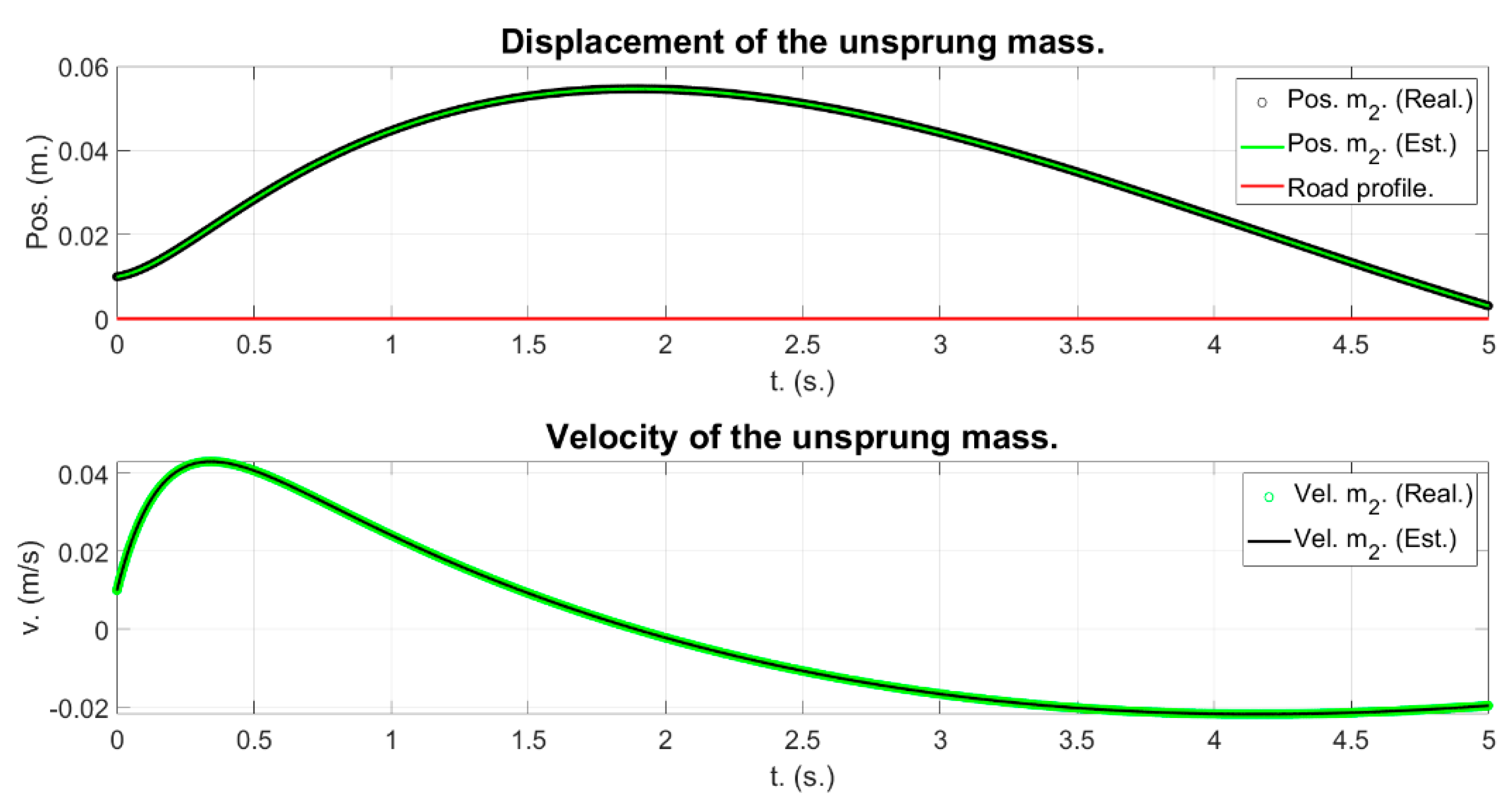
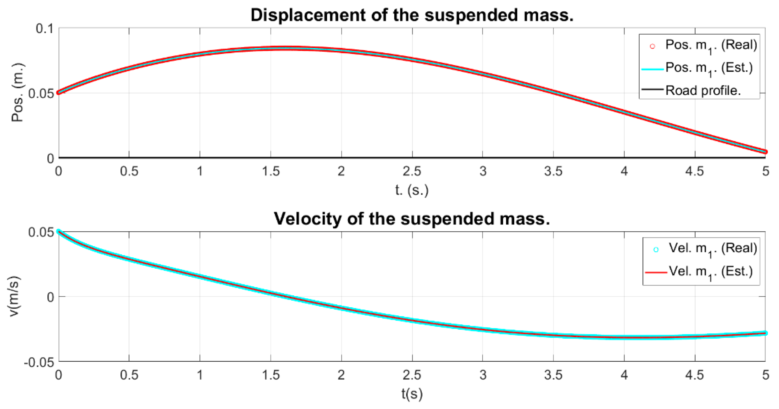
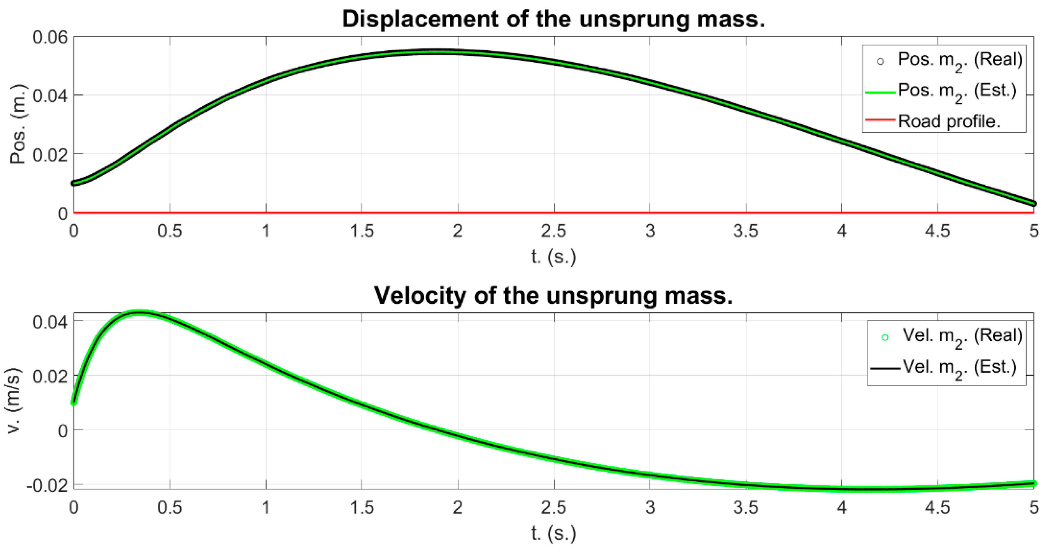
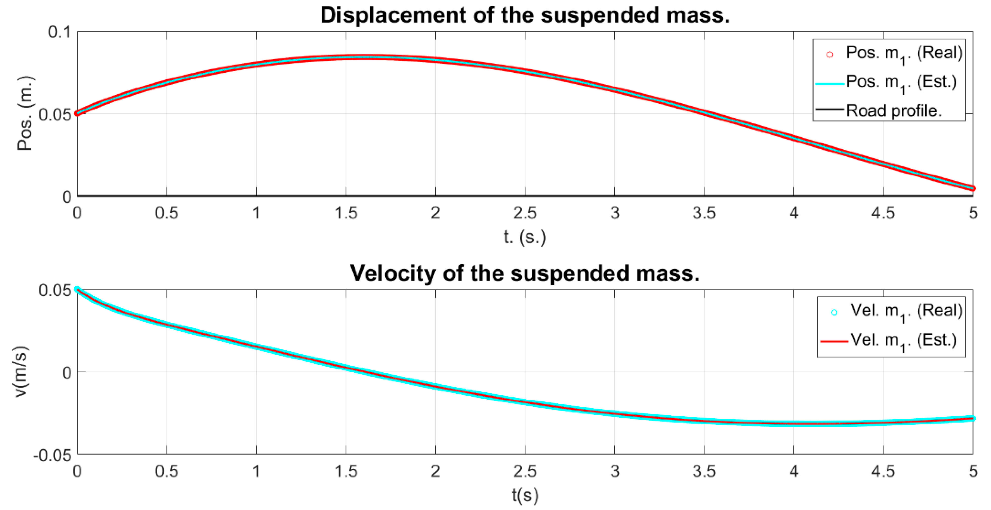
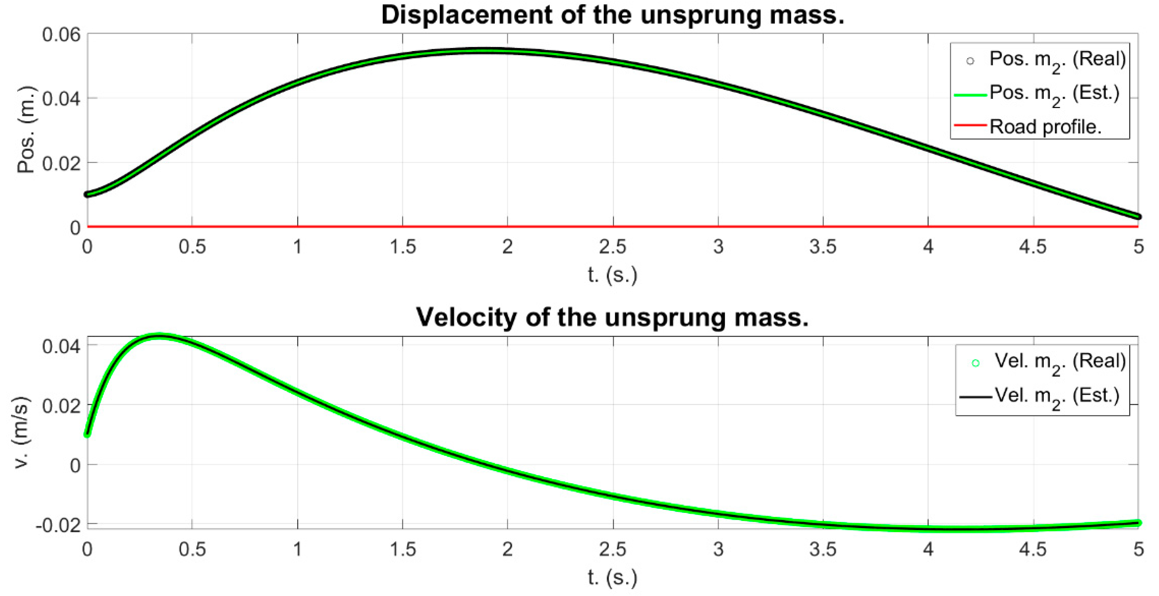
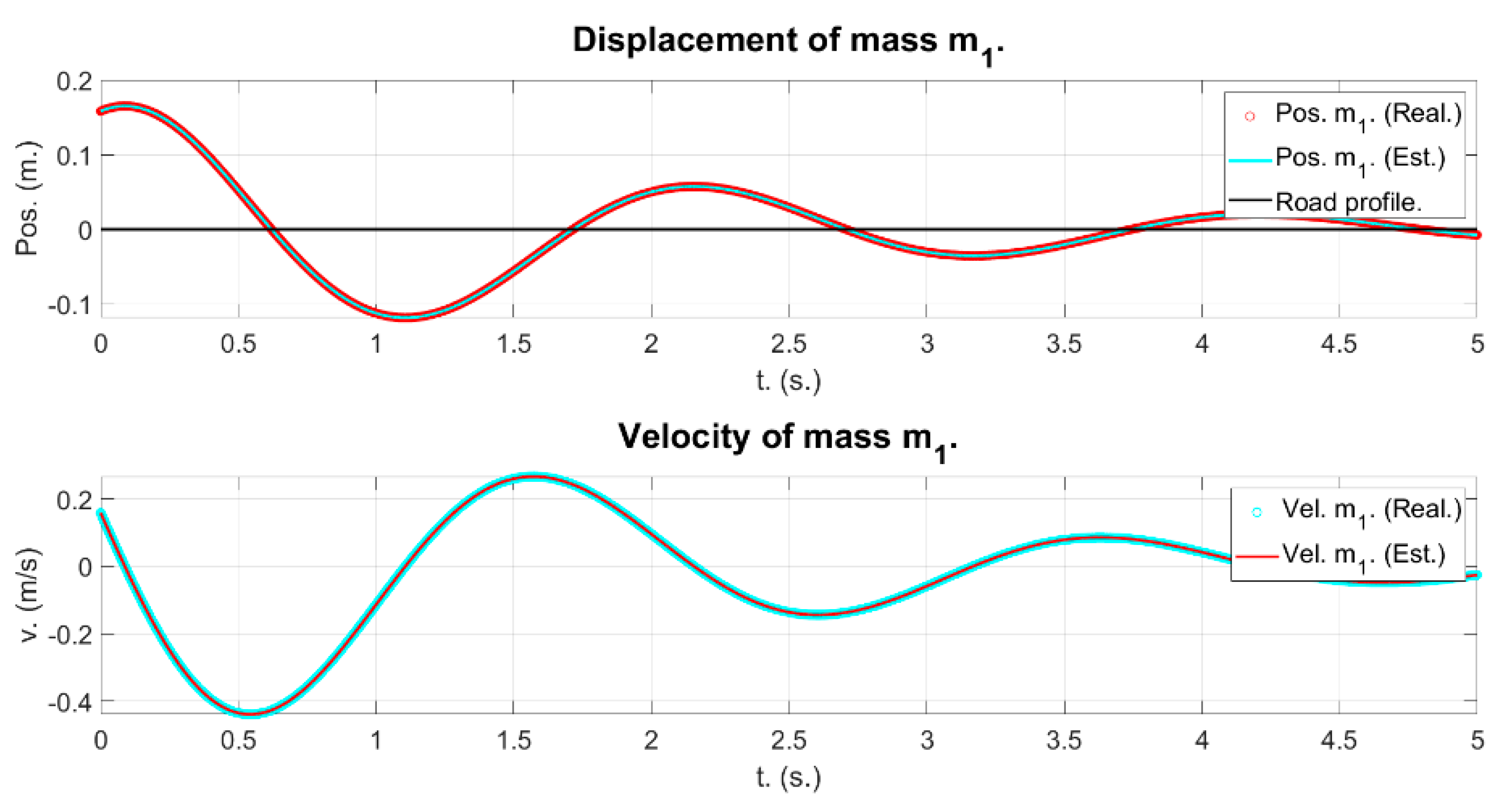
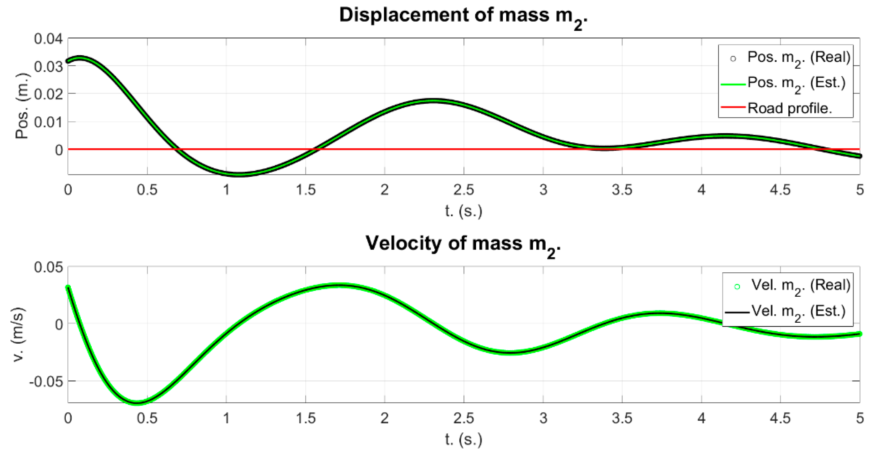
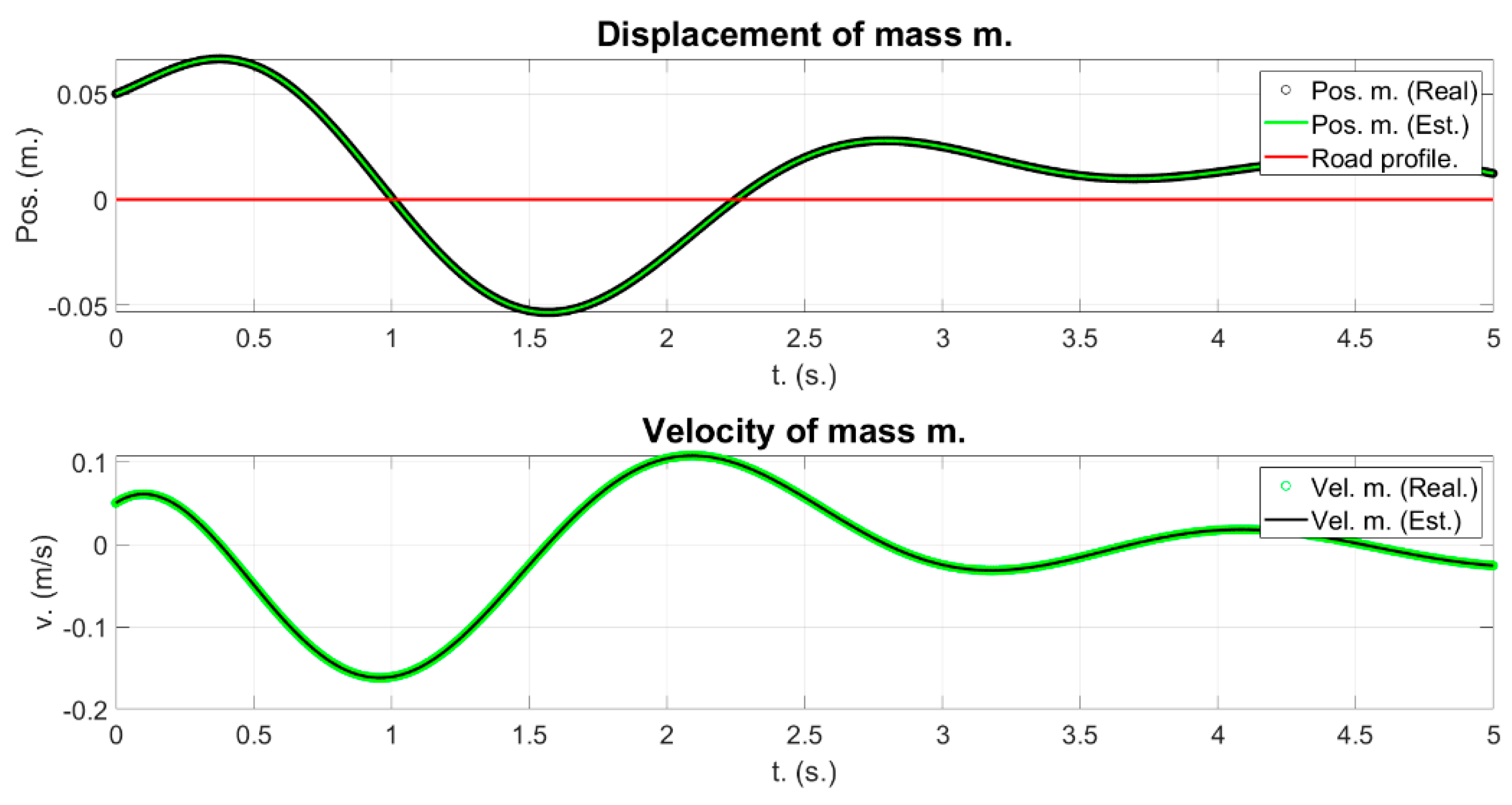
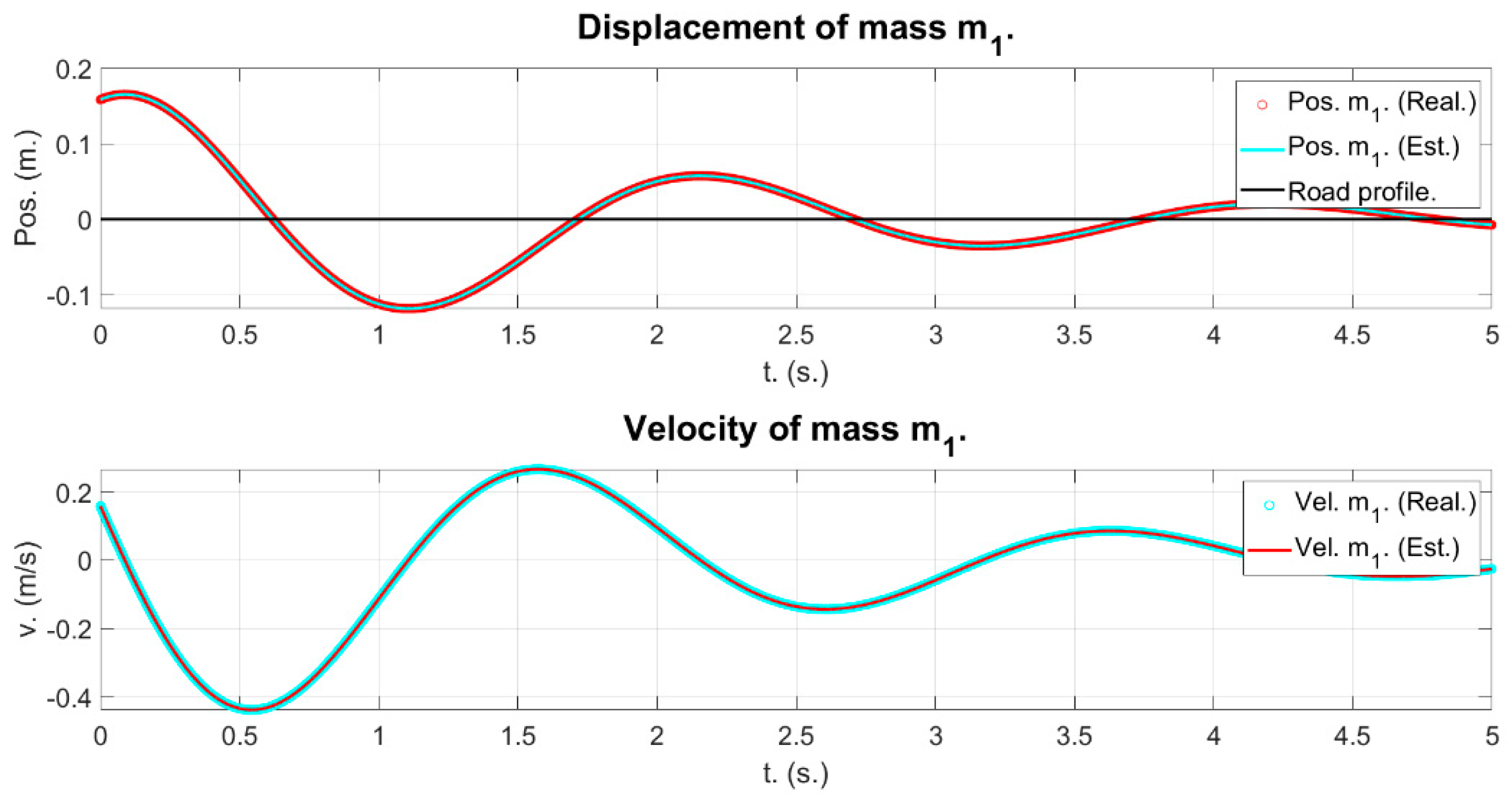
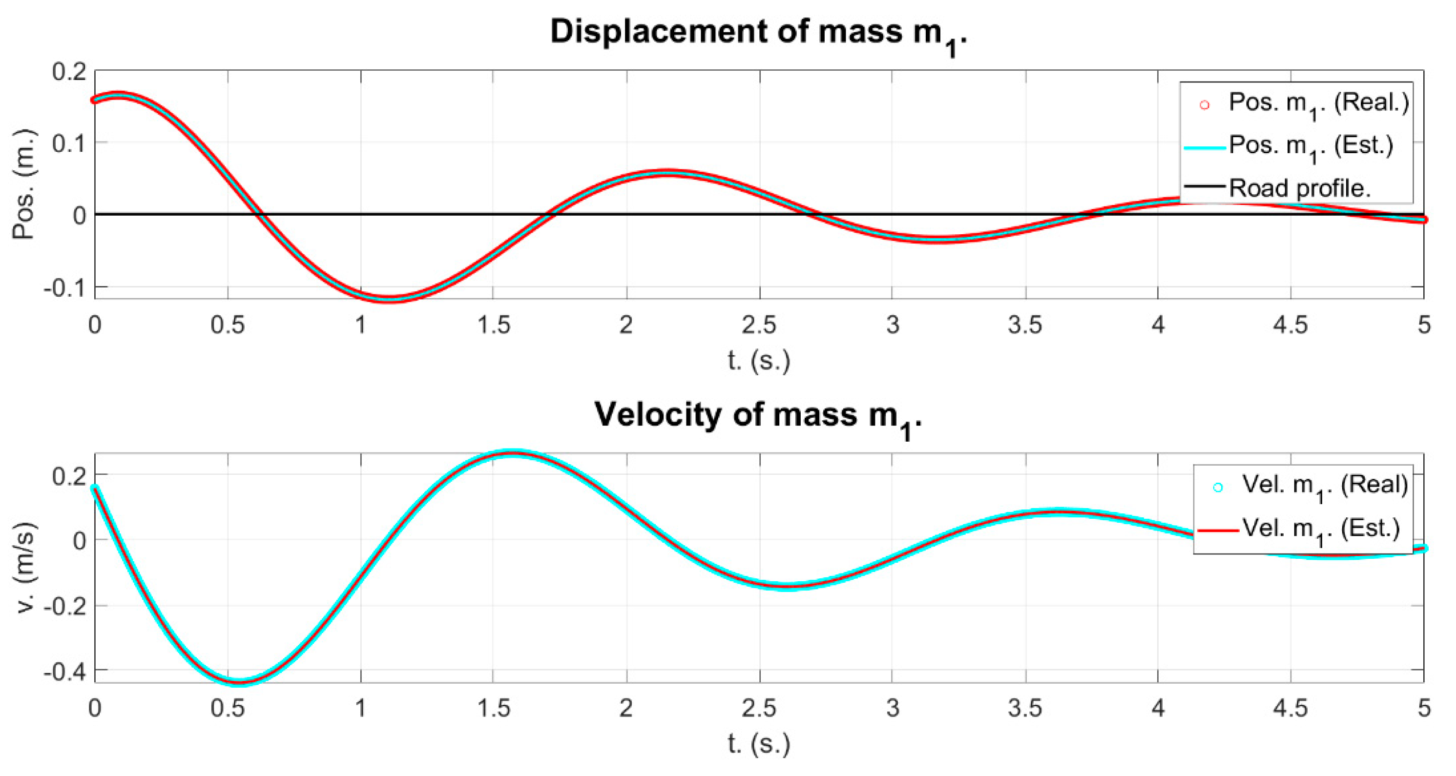
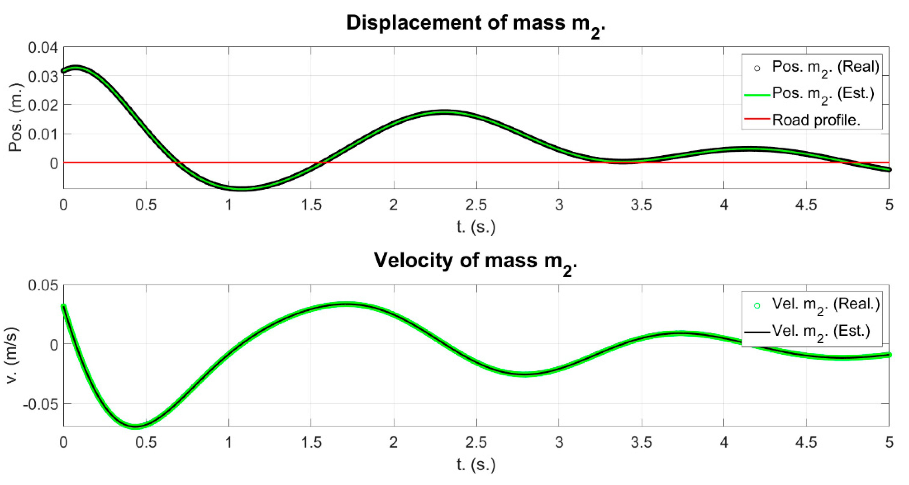
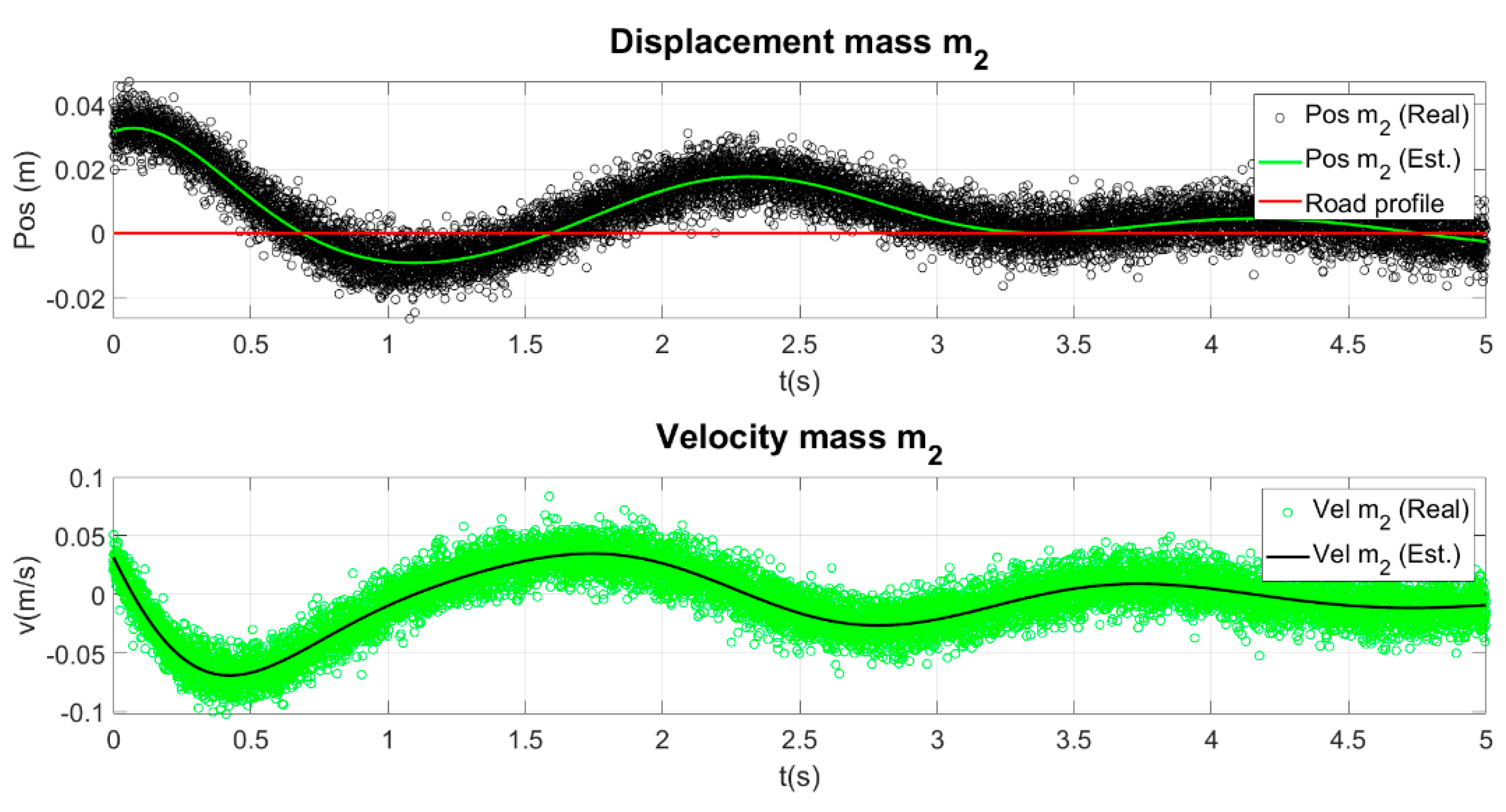
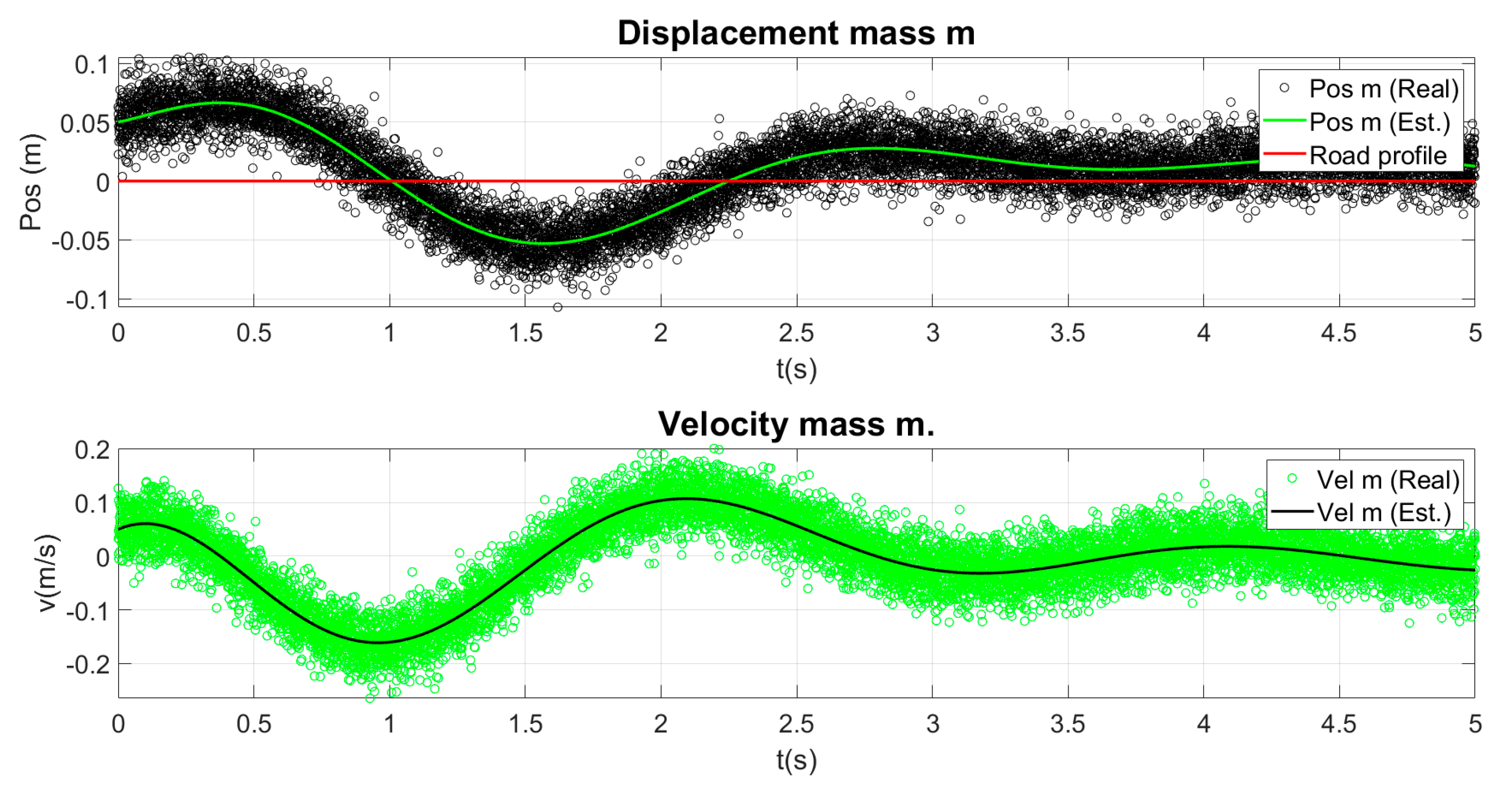
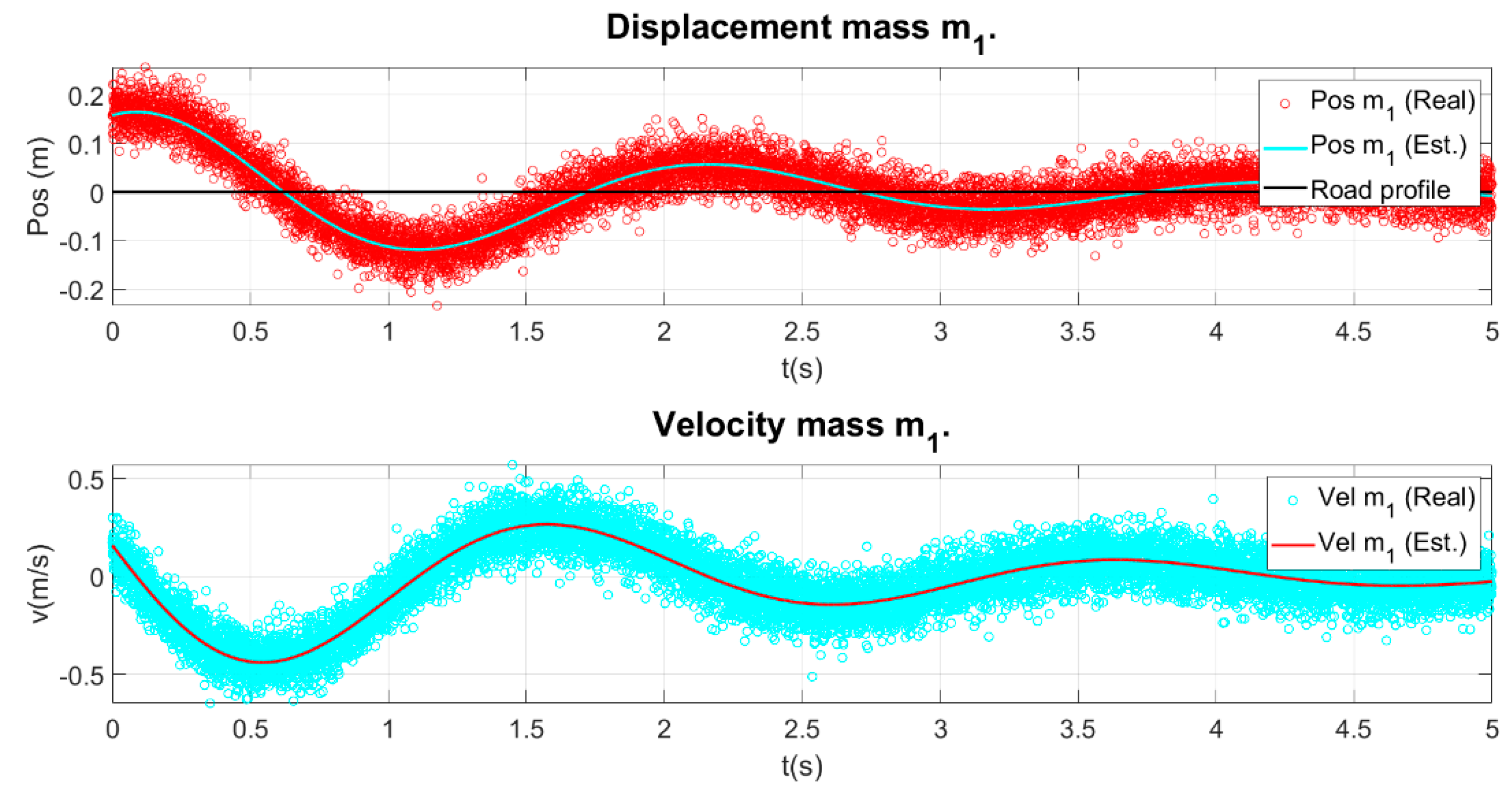
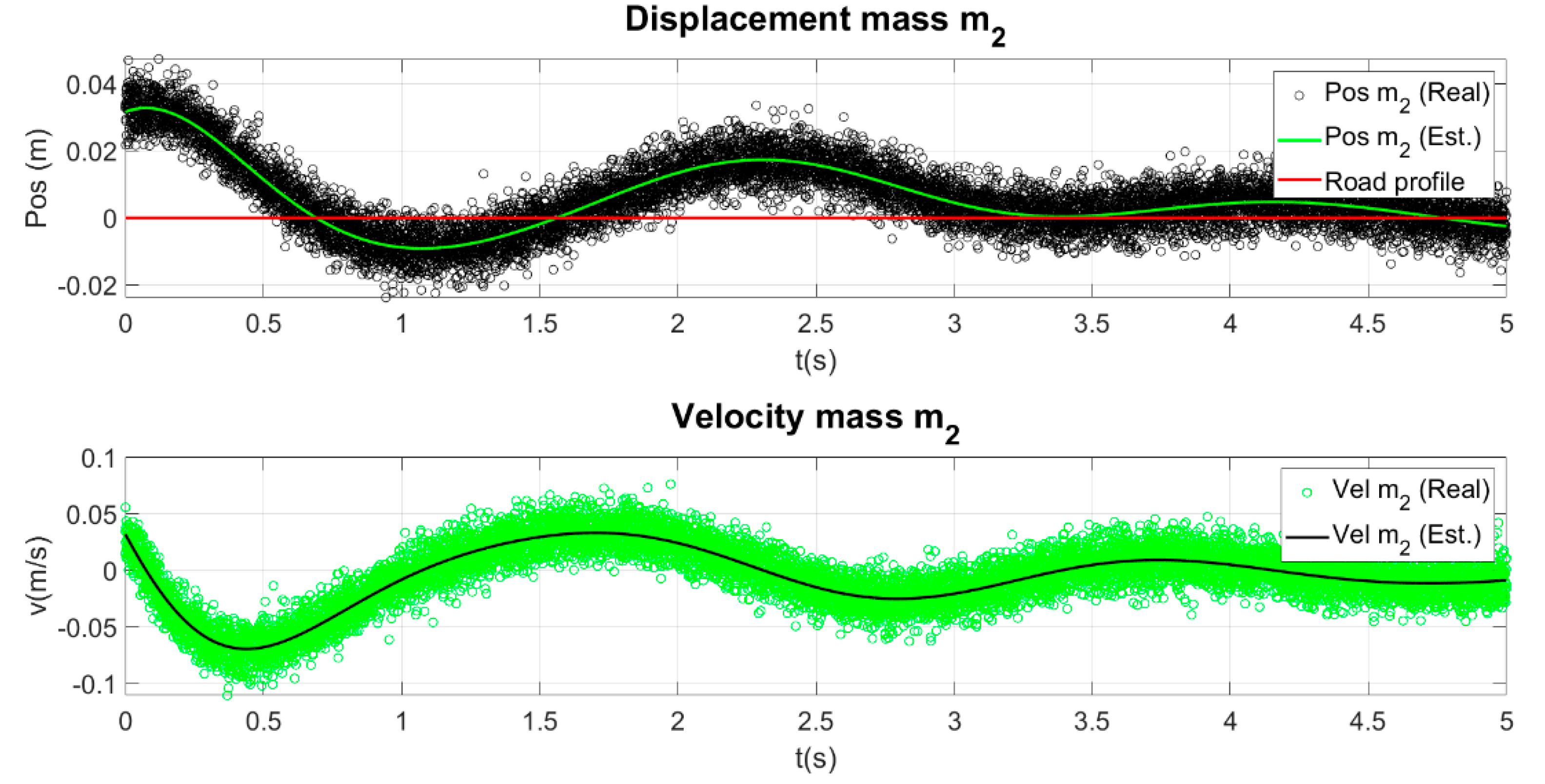
For the full quarter-vehicle model, the same results were obtained, namely, the unrestricted optimization problem provided us with erroneous identified suspension parameters (
Figure 21,
Figure 22,
Figure 23 and
Figure 24), whereas the restricted problem (leaving the masses fixed), provided us with perfectly identified ones, as shown in
Figure 25,
Figure 26,
Figure 27 and
Figure 28. The error could not be detected by looking at the curve comparison. Again, the restriction was performed by setting the masses as global variables. Again, this happened with all the tests detailed in
Table 6.


