1. Introduction
In practical engineering systems, different kinds of noise and various unmeasurable inputs or disturbances are often present in the system state equation and measurement equation due to environmental influences, improper selection of model parameters, equipment failures, etc. When dealing with the state estimation problems of the above systems, expert scholars usually refer to these disturbances or inputs that cannot be measured and for which no priori information is known collectively as unknown inputs [
1,
2,
3,
4,
5]. The algorithms for state estimation of nonlinear systems containing unknown inputs are now widely used in many application fields such as autonomous navigation [
6], target tracking [
7], fault-tolerant control [
8], and fault detection [
9].
For nonlinear stochastic systems where the unknown input occurs only in the state equation, Ref. [
10] presented an extended Kalman filter algorithm with unknown inputs for continuous-time systems that can identify the structural parameters and states of the system in real time. For discrete-time systems, Ref. [
11] proposed an unknown input extended Kalman filter, which builds on the extended Kalman filter (EKF) [
12] by completely decoupling the unknown inputs without forcing the measurement equation to be linear. However, the EKF algorithm requires linearization of the system, which inevitably introduces linearization errors and can lead to degraded filtering performance or even filter divergence when the system is strongly nonlinear. To this end, a nonlinear recursive filter is given in [
13], which obtains unknown inputs for signals of arbitrary type via least-squares unbiased estimation and transforms the state estimation problem into a standard unscented Kalman filter (UKF) [
14,
15] problem. Since the unscented transform enables the posterior probability density function of Sigma points after propagation through a nonlinear function to reach at least the second-order term of the Taylor series expansion, its filtering accuracy is higher than that of the EKF, while overcoming the shortcoming that the EKF is only applicable to weakly nonlinear systems. In addition, Ref. [
16] introduced statistical linearization and weighted least squares to estimate the unknown inputs and proposed a robust strong tracking unscented Kalman filtering algorithm with unknown inputs. However, UKF is prone to nonlocal effects of sampling when dealing with high-dimensional nonlinear systems, which leads to numerical instability in the filtering process and degradation of the filtering performance. Later, by improving the cubature Kalman filter (CKF) [
17] algorithm, Ref. [
18] designed a distributed filter that estimates the state and unknown inputs simultaneously. With further research, a nonlinear unknown input observer (NUIO) was proposed in [
19] based on singular value decomposition-assisted dimensionality reduction CKF. The method preserves the third-order accuracy of Taylor expansion integral of the nonlinear state function by sampling the nonlinear part of the nonlinear state function instead of all of it.
However, the types of algorithms mentioned above only consider the case where the system state equation contain unknown inputs. With further research, some scholars have extended such filtering algorithms to the case where the measurement equation of the system model also contain unknown inputs. To address the problem of filter design for such direct feedthrough nonlinear systems, an unknown-input generalized extended Kalman filter is proposed in [
20] for continuous-time systems. For discrete-time systems, an adaptive three-stage Kalman filter capable of tracking faults and unknown inputs is proposed in [
21], which can be used in situations where faults and unknown inputs are not fully known, and its stability is demonstrated. Later, Ref. [
22] proposed a robust EKF to estimate both the unknown inputs and the system states simultaneously. Ref. [
23] proposed a novel adaptive three-level EKF for the problem of severe performance degradation of the conventional Kalman filter in handling unknown inputs, while a three-level UKF and robust three-level UKF were given in [
24] to solve the unknown inputs and state estimation for nonlinear systems where the unknown input information is not completely known. In addition to this, many other scholars have considered the impact of uncertainties on system filtering caused by systems with both unknown inputs, missing measurements and multiplicative noise, and have carried out extensive research [
25,
26,
27,
28,
29].
The above filtering algorithms all consider the case where the unknown input signals are the same in both state and measurement equations, but in practical application systems, the unknown input signals in the two equations are often different. For such systems, Ref. [
30] designed a decoupling filter and an adaptive minimum upper filter to obtain optimal and suboptimal estimation of the state via introducing an adaptive adjustment factor, but this skips the estimates of the dual unknown inputs and does not give an explicit iterative formula for the estimates of the dual unknown inputs. Ref. [
31] proposed a CKF-based NUIO method for robust sensor fault detection and demonstrated the superiority of this method compared to the NUIO methods of EKF and UKF. However, some scholars have found that constant rounding errors in CKF during iteration make the covariance matrix asymmetric or non-positive definite, which leads to degradation of filtering performance or even divergence. Later, Ref. [
32] proposed a square-root cubature Kalman filter (SRCKF) based algorithm for battery charge state estimation. Since SRCKF directly propagates and updates the state covariance matrix square root by means of Cholesky decomposition, ensuring the non-negativity of the covariance matrix and avoiding the divergence of the filter.
To sum up, the research on state estimation for nonlinear systems containing unknown inputs has achieved the above fruitful results, and a SRCKF algorithm outperforms CKF and UKF algorithms with regard to computational efficiency, filtering accuracy, and numerical stability, but the existing nonlinear filtering estimation algorithms with unknown inputs still have many limitations: (i) the traditional SRCKF algorithm has degraded filtering accuracy or even divergence when dealing with unknown inputs; (ii) existing nonlinear filtering algorithms consider unknown inputs, but assume that the unknown inputs in the state equation and measurement equation are the same, which narrows the applicability of the filter; (iii) only the estimation of the state can be achieved—the estimation of the unknown inputs cannot be obtained.
Based on the above analysis, this paper proposes two new, improved square-root cubature Kalman filter algorithms. Compared with the existing results, the main contributions have the following three aspects:
- (1)
When the state and measurement equations contain different unknown input signals without any prior information regarding the dual unknown inputs, according to the MVUE criterion, by designing the innovation to deal with the state and the dual unknown inputs, the traditional SRCKF is improved and extended to the nonlinear system with dual unknown inputs, which solves the problem that the performance of the SRCKF algorithm is seriously degraded or even cannot be applied in this case.
- (2)
The MVUE of the state and dual unknown inputs is obtained by minimizing the trace of the estimation error covariance matrix and then solving for it using Schur’s complement lemma, provided that the undetermined gain matrix satisfies certain constraints.
- (3)
The ISRCKF does not require the unknown inputs in the state and measurement equations to be the same quantity, and the system under consideration is more in line with the practical application context, which is applied more loosely and with a wider range of applicability.
This paper is structured as follows.
Section 2 gives a description of the research problem. In
Section 3, an ISRCKF1 algorithm with dual unknown inputs is proposed. In
Section 4, the simpler ISRCKF2 algorithm with dual unknown inputs is redesigned. In
Section 5, we give a nonlinear example to study the validity of the two algorithms and compare the estimation results of the two algorithms with the SRCKF algorithm to prove the performance of the proposed algorithm. In
Section 6, we provide our conclusion.
2. Problem Description
Consider the following direct feedthrough nonlinear discrete stochastic systems with dual unknown inputs:
where
and
represent the state vector and the measured output vector of the system, respectively;
and
are nonlinear transfer functions,
is the known control input signal,
and
are unknown input vectors in the state and measurement equations, respectively;
and
are the process and measurement noise of the system, respectively, which are zero-mean Gaussian white noise signals that are not correlated with each other, and their nonsingular covariance matrices
and
are known;
and
are determined matrices of suitable dimensional coefficients; the initial state value
follows a Gaussian normal distribution and is independent of
and
; the unbiased estimate
of
and the initial covariance matrix
are known; let
be an unbiased estimation of
, then
is an unbiased estimation of
, but a biased estimation of
due to unknown inputs.
Assumption 1. Assuming that the output, like most industrial systems, is linear and does not lose generality [19,31]. However, the EKF is a linearization of both state and measure equations using Jacobi matrices; in nonlinear situations, the output Function (2) can be linearized around the operating points as follows:where is the matrix of linearized measurement coefficients. Remark 1. We generally default that systems (1)–(3) satisfy the state observability condition, and the specific research on parameter observability can refer to [33]. Assumption 2. The matrix has full rank, that is, .
Remark 2. Assumption 2 is the basic condition for decoupling the unknown inputs in the state and the measurement equations, requiring that the measurement vector dimension must be greater than the sum of the dual unknown input vectors, otherwise there is not enough information to estimate the dual unknown input vectors [11,13]. When Assumption 2 holds, the following four conclusions hold simultaneously. - (i.)
.
- (ii.)
.
- (iii.)
There is no linear dependence between columns of and columns of .
- (iv.)
.
Remark 3. The above optimal filtering problem for the system is to obtain stepwise recursive unbiased optimal filtering sequences , and for the dual unknown inputs and the system state based on the time series of measurements , provided that the initial state and its unbiased estimates and covariance matrix are known.
3. ISRCKF1
Consider the case where the unknown input signals in the equation of state and the measurement equation are different, i.e.,
. For the system models (1)–(3), using the idea of innovation feedback, this section will give the ISRCKF filter for estimating the system state and the dual unknown inputs. The one-step estimate
of
, the prediction error covariance matrix
, and its square-root
are first obtained from the known measurement sequence
, the initial state estimate
and the covariance matrix
. The specific steps are given in
Section 3.1; then solve for the undetermined gain matrix
to obtain the estimate
of
. The specific expression and detailed derivation steps are given in
Section 3.2. Based on the obtained unknown input estimate
, design the estimator
for
. The specific expression for the filter gain
to be determined and the detailed derivation steps are given in
Section 3.3; further, based on the obtained dual unknown input estimates
and
, the estimator
for
is designed and the gain matrix
scan be obtained by minimizing the trace of the covariance
when performing the state update, as given in
Section 3.4. Finally, update the square-root
of
, given in
Section 3.5.
3.1. Time Update
where
denotes the square-root of
and is obtained by performing Cholesky decomposition on
. It should be noted that in this paper, the above covariance is factorized only at the initial moment, i.e., the Cholesky decomposition is performed for the known initial covariance
at
k = 1.
- 2.
Calculate the cubature points
where
is the cubature point and
is the optimal unbiased estimate of
when the measurement time series
is known;
is the number of cubature points and twice the dimension
of the state
, that is,
;
is the set of
cubature points with the same weight based on the third-order spherical radial criterion,
is the
ith column of the point set
, and the point set
can be expressed as
- 3.
Calculate the nonlinear propagated cubature points and the one-step state estimation
where
denotes the updated cubature points;
is the weight corresponding to the cubature points.
- 4.
Calculate the square-root of the prediction error covariance matrix
where
denotes triangular decomposition,
is a lower triangular matrix, and
is the square-root of
, which can be acquired by performing Cholesky decomposition on
, i.e.,
.
The central weighting matrix
is given by
- 5.
Evaluate the prediction error covariance matrix
where the expression for
is given in Equation (7). The detailed derivation of Equation (11) can be found in [
17]. Without affecting the calculation results, for ease of writing, we will simply abbreviate
as
from here on.
3.2. Estimation of Unknown Input
Designing the innovation
, according to the system models (1)–(3), the innovation at moment k is expanded as follows:
where
and
are given by the following equations, respectively:
From the known conditions we get
Using the innovation feedback
, the unbiased estimate
for design
is as follows:
The next step is to calculate the gain matrix
. From Equations (12) and (16), we can obtain the estimation error of the unknown input
:
Theorem 1. If the system equation satisfies , then for any and , Equation (16) is the minimum variance unbiased estimator of , if and only if the following equation holds:where .
Proof. First, we give the necessary conditions for Equation (18) to hold as follows:
Equation (19) can be expanded to
and
, at which point Equation (17) can be simplified as
Thus combining Equations (15) and (20), regardless of the values taken by and , is an unbiased estimate of the unknown input . Unbiasedness is proven.
Further based on Equations (11), (13), and (20), the covariance matrix
of
can be approximated, that is,
We choose the pending gain matrix
to minimize the
variance by satisfying the unbiased condition of Equation (19), so for solving
we can choose Equation (22) applied using the Lagrange multiplier method, which can be found in [
1] for a more detailed description of the method.
Similar to the proof of Gillijns in [
34], the Lagrange multiplier method is adopted to solve the extreme value problem under this constraint. The Lagrangian is given by
where
is the Lagrange multiplier matrix,
, and the factor “2” is intended to keep the calculation simple.
Taking the derivative of Equation (23) with respect to
and making the resulting derivative zero, we get
The system of linear equations consisting of Equations (24) and (19) is as follows:
According to the literature [
34], the coefficient matrix of the system of equations (25) is nonsingular when
is invertible, at which point the linear system equation has a unique solution. Finally, using the Schur complement lemma, the gain matrix
expression (18) is obtained. The proof is completed. □
3.3. Estimation of Unknown Input
Using the estimate
of the unknown input
obtained in the previous section, design a new innovation feedback as follows:
According to Equation (26), the unbiased estimate
of the unknown input
is designed as follows:
Then, by combining Equations (12), (14), and (27), we can get the estimation error of the unknown input
:
Theorem 2. If the system equation satisfies , then for any and , Equation (27) is the minimum variance unbiased estimator of , if and only if the following equation holds:where .
Proof. First, we give the necessary conditions for Equation (29) to hold as follows:
From Equation (30), rewrite the expression for
, that is,
According to Equations (15) and (31), , so unbiasedness is proven.
Then, from Equations (11), (13), and (31), the covariance matrix
of
is obtained as
Finally, by solving the following conditional extremum problem, Expression (29) of the undetermined gain matrix
, which holds Equation (30) and minimizes trace of
, is calculated, and then the minimum variance unbiased estimate
of
and the corresponding minimum covariance
are obtained:
This proof is similar to the proof of Theorem 1 above and therefore omitted. □
3.4. Estimation of State
First, we consider updating the one-step estimate
. Compensating for
by adding
obtained in the previous section, we can get the updated one-step estimate
as follows:
From Equations (1) and (34), the estimation error of the updated one-step estimate
is obtained:
Further, the covariance matrix is approximated from Equation (35):
where the expression
is given in Equation (11) above and the specific derivations for
,
, and
are given by Equations (38) and (39).
First, the unknown input prediction estimation error at moment
k is defined as
Combining Equations (11), (13), (20), (31), and (37), it is obtained that
where the expressions for
and
are given in Equations (11) and (30), respectively. Further,
is obtained.
From
, combined with Equation (37) we get
where
is given in Equation (32) above. In summary,
,
, and
are derived.
Then, update the innovation based on the estimated values
and
of the unknown inputs
and
already obtained above:
Further, we can design the estimated value of state
as follows:
From Equations (3) and (41), the estimation error of state
is obtained:
where
is given in equation (35) above.
Remark 4. In Section 3.2 and Section 3.3, we have proved that and are both unbiased estimates. Combining Equations (42), (35), (13), and (15) yields , that is, the state estimate obtained from Equation (41) is the unbiased estimate of for any value of . Therefore, we only need to calculate the undetermined gain matrix next, which minimizes the trace of the state estimation error covariance matrix . It should be noted that for state estimation, references [
35,
36,
37]
have also conducted research on state and parameter estimation for measurement scarcity and bilinear systems. The covariance matrix of the estimation error is given by the following equation, and the specific derivation process can be seen in
Appendix A:
where
,
, and
are given by Equations (36), (21), and (38) above.
Theorem 3. Under the condition that is positive definite, the undetermined gain matrix which minimizes the trace of is given by Proof. The gain matrix
is obtained by minimizing the trace of
, which leads to the state estimation filter, that is, solving for the following equation:
By substituting Equation (43) into Equation (45), and then combining the trace derivative rule of the matrix, we get
Finally, the collation leads to Equation (44). The proof is completed. □
3.5. Update the Square-Root
This section calculates the square-root
of
. Unlike the traditional SRCKF, the undetermined gain matrix
in expression
is obtained under the minimum variance unbiased estimation criterion, that is,
in
Section 3.4.
- 2.
Calculate the nonlinear propagated cubature points and the predicted measurement
- 3.
Calculate the square-root of the estimation error covariance matrix
where the central weighting matrices
and
are expressed as
3.6. Summary of ISRCKF1 Iteration Steps
To demonstrate the proposed filter design process more conveniently, the iterative steps of ISRCKF1 will be summarized in this section to give the dual unknown input and state estimation algorithm based on ISRCKF1 as follows:
Step 1: Initialization
where
denotes the square-root factor of
and is obtained by performing Cholesky decomposition on
. Set time
k = 1.
Step 3: Estimation of unknown input
Step 4: Estimation of unknown input
Step 5: Estimation of state
Step 6: Update square-root
Step 7: Set time k = k + 1 and return to step 2.
4. ISRCKF2
In practice, the above ISRCKF1 needs to be updated gradually with innovation and the iterative process of the algorithm is cumbersome, making the solution process time-consuming and costly. In this section, we rederive a more concise filter for the system studied above, utilizing the same innovation feedback. Given
,
, and
, the filter first obtains
,
, and
. The detailed derivation is the same as
Section 3.1, and will not be repeated here; when the measurement is updated to step k, the filter estimate
of
is obtained. The derivation and the specific expression for
are given in
Section 4.1; the next step is to obtain filter estimates
and
for the dual unknown inputs
and
. The derivation and the specific expressions for
and
are given in
Section 4.2; finally, the square-root
of
is updated, and its detailed derivation is the same as
Section 3.5, which will not be repeated here.
4.1. Minimum Variance Unbiased Estimation of State
This section calculates the filter undetermined gain matrix such that is the minimum variance unbiased estimate of .
First, the innovation feedback
is used to correct the one-step estimate
to obtain the unbiased estimate
of
and the corresponding covariance matrix. For systems (1)–(3), the innovation at time
k can be expanded as shown in Equation (12) above. Using the innovation feedback, the filtered estimate of
can be obtained as follows:
Then, calculate the gain matrix
. From Equations (1), (12), (14), and (53) we get
According to Equation (13), Equation (54) can be transformed into
Remark 5. It should be noted that the precondition for obtaining Equation (55) from Equation (54) is that the pseudoinverse matrix exists, which is indeed a limitation of ISRCKF2 and a problem that we will address in future research.
Theorem 4. If the system equation satisfies , then for any and , Equation (53) is the minimum variance unbiased estimator of all possible , if and only if the following equation is true: Proof. First, we give the necessary conditions for Equation (56) to hold as follows:
If Equation (57) holds, it is equivalent to
and
. Substituting into Equation (54) gives
Combining Equation (15) yields . Thus, the state estimate obtained from Equation (53) is the unbiased estimate of for any value of , regardless of the values of and . Unbiasedness is proven.
Further from Equations (11), (13), and (58),
can be approximated, that is,
Then, the undetermined gain matrix
is solved by solving the following constrained optimization problem.
Let the Lagrangian be
where
is the Lagrange multiplier matrix,
, the factor “2” is intended to keep the calculation simple.
Taking the derivative of Equation (61) with respect to
, and making the resulting derivative zero, we get
The system of linear equations consisting of Equations (62) and (57) is as follows:
Finally, using Schur’s complement lemma to solve the above equations, Equation (56) is obtained. The proof is completed.□
4.2. Minimum Variance Unbiased Estimation of Unknown Inputs
This section considers the estimation of
and
, where the estimation of
is obtained in
Section 4.2.1, and also determines the conditions that need to be satisfied for the undetermined gain matrix
.
Section 4.2.2 obtains the estimation of
and determines the conditions that need to be satisfied for the undetermined gain matrix
.
4.2.1. Estimation of Unknown Input
In this subsection, based on the innovation feedback from the previous section, the gain matrix will be calculated.
First, using the innovation
, design the unbiased estimate
of
as follows:
Then, from Equations (12) and (64), the estimated error of the unknown input
is obtained:
Theorem 5. If the system equation satisfies , then for any and , Equation (64) is the minimum variance unbiased estimator of , if and only if the following equation is true: Proof. First, we give the necessary conditions for Equation (66) to hold as follows:
Equation (67) can be transformed into
and
. At this point, Equation (65) can be simplified as
Therefore, from Equations (15) and (68), we get . Unbiasedness is proven.
Further, from Equations (11), (13), and (68), the covariance matrix
of
is calculated:
Finally, solving the following constraint problem yields the undetermined gain matrix
, which leads to the minimum variance unbiased estimate
of
and the corresponding minimum variance matrix
.
Similar to the proof of Theorem 4, let the Lagrangian be
where
is the Lagrange multiplier matrix,
, the factor “2” is intended to keep the calculation simple.
Taking the derivative of Equation (71) with respect to
, and making the resulting derivative zero, we get
The system of linear equations consisting of Equations (72) and (67) is as follows:
Using Schur’s complement lemma to solve the above equations, Equation (66) is obtained. The proof is completed. □
4.2.2. Estimation of Unknown Input
Since the innovation feedback
used in ISRCKF2 is the same as the innovation
designed for the estimation of
in
Section 3.2, this subsection follows the same proof procedure as in
Section 3.2 and will not be repeated here.
4.3. Summary of ISRCKF2 Iteration Steps
In order to clearly reflect the filter design process with simplified dual unknown inputs, this section will summarize the steps of ISRCKF2 and give a more concise iterative process as follows:
Step 1: Initialization
where
denotes the square-root factor of
and is obtained by performing Cholesky decomposition on
. Set time k = 1.
Step 3: Estimation of state
Step 4: Estimation of unknown inputs
and
Step 5: Update of square-root
Step 6: Set time k = k + 1 and return to step 2.
5. Simulation Results
To demonstrate the effectiveness of the two filtering algorithms proposed in this paper, in this section, the ISRCKF algorithm is compared with the SRCKF algorithm proposed in [
32]. First, the simulation uses a fifth-order two-phase nonlinear model of the induction motor [
38,
39], which can be described using the system models (1)–(3) as follows:
where
denotes the stator currents a and b, the rotor fluxes a and b and the angular speed, respectively,
represents the stator voltages control vector,
is the number of pole pairs and
is the load torque.
The rotor time constant
and the parameters
,
and
are defined as follows:
where
and
are the per-phase resistances of the stator and rotor,
and
are the per-phase inductances of the stator and rotor, and
is the rotor moment of inertia.
The simulations are carried out with the same numerical values as in [
38], that is,
,
,
,
,
,
,
,
and
.
The motor control input signals are and .
The system correlation coefficient matrix is as follows:
The covariance matrices for
and
are given by
ISRCKF1 and ISRCKF2 are set in the simulation the same system and filter initial conditions as the comparison algorithm, referring to [
39], that is,
,
,
,
,
,
,
.
Setting the unknown input in the equation of state equal to , and the unknown input in the measurement equation equal to .
To quantitatively compare various nonlinear filtering algorithms, the root mean square error of
at moment k is denoted by
, which is defined as follows:
where
denotes the number of Monte Carlo simulations and
is set in the simulation;
and
denote the actual and estimated values of the state
at moment k under the nth Monte Carlo simulation, respectively. For unknown inputs
and
, the above equation is also used as a quantitative evaluation index.
In the following, the validity of the proposed ISRCKF1 and ISRCKF2 for the system containing dual unknown inputs is verified, and to ensure the accuracy and generality of the experimental results, the number of sampling steps N is taken as large as possible, and the same as in [
39] is set to be N = 1800.
Case 1: When the unknown inputs in the state and measurement equations are the same input signal, that is,
, the state estimation performance difference of each filtering algorithm is considered. After 100 Monte Carlo simulations, the mean RMSE of ISRCKF1 and ISRCKF2 with dual unknown inputs and states between moments 0~1800 are shown in
Table 1,
Table 2,
Table 3,
Table 4,
Table 5 and
Table 6. It should be added that “N/A” in the table means that the algorithm is not applicable. The time evolution curves of the state RMSE for the proposed filtering algorithms are shown in
Appendix B.
Figure 1 and
Table 1 show the estimation results of
when considering the unknown input as sine and cosine electrical signals. It can be seen that the filtering algorithm given in this paper can track and estimate the unknown input
better, and the ISRCKF2 estimation accuracy is higher.
Figure 2 and
Table 2 show the estimation results of
. We can also conclude that the filtering algorithm proposed can better track and estimate
, and the estimation of ISRCKF2 produces a smaller mean RMSE.
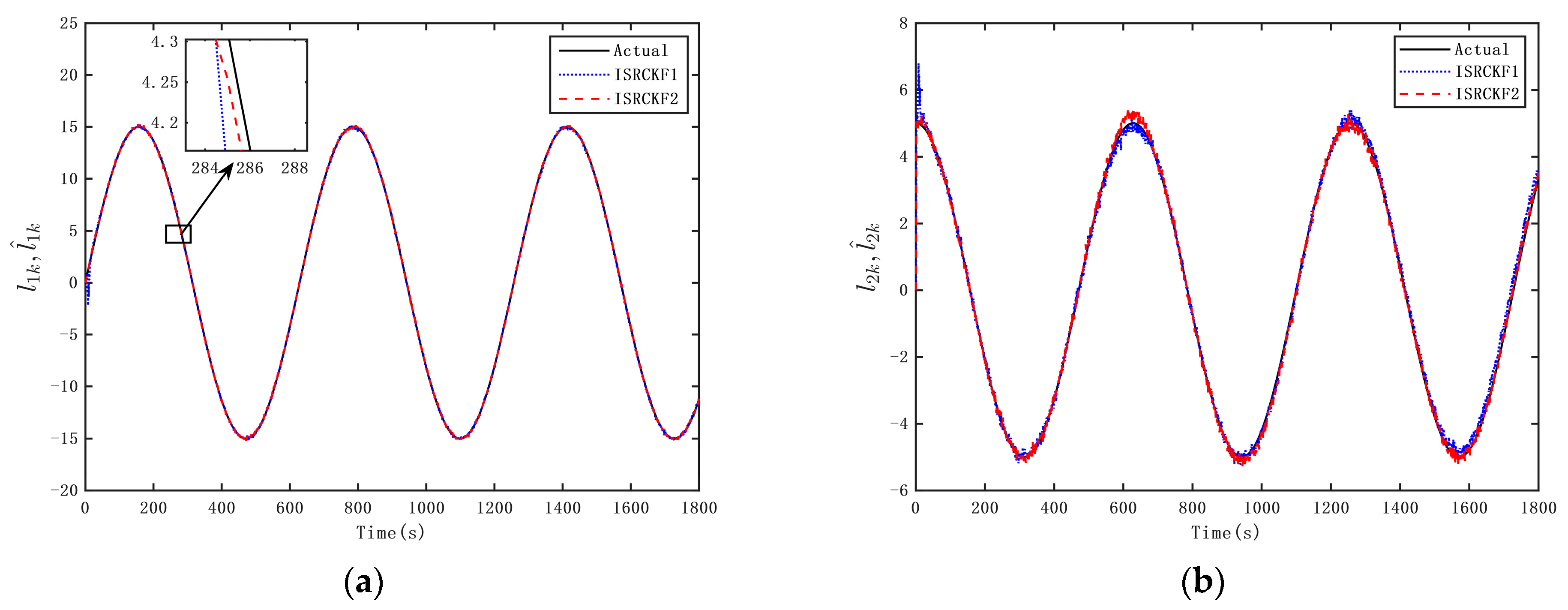
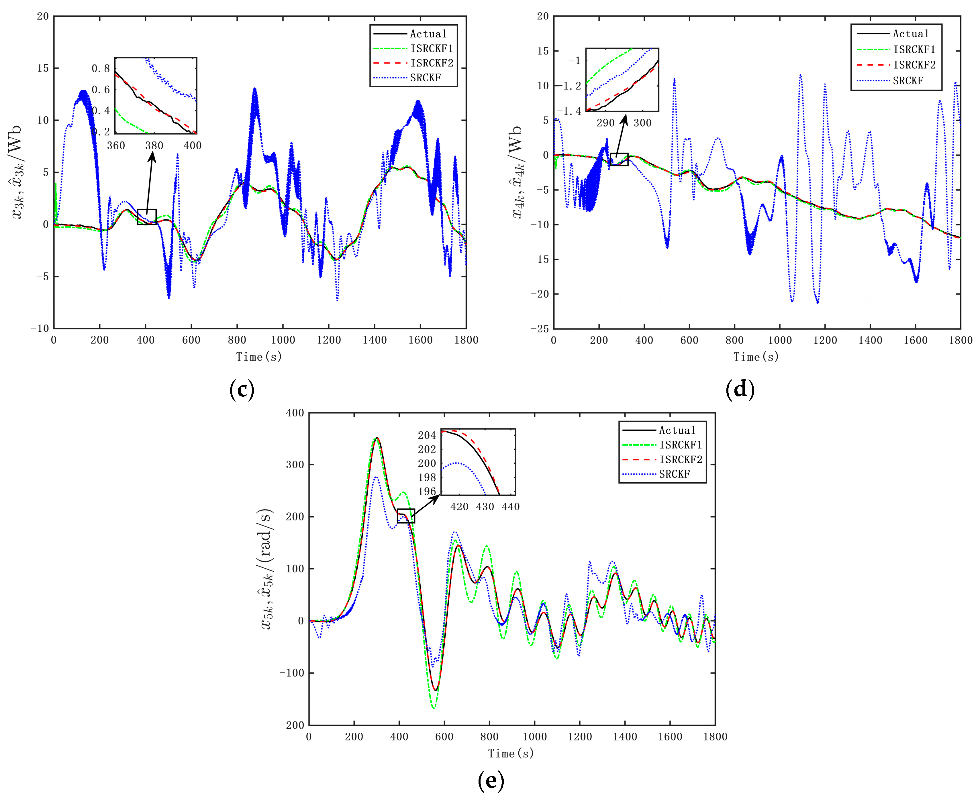
Figure 3 and
Table 3 show the estimation results of the system states
. From
Figure 3, we can see that the overall filtering performance of the proposed ISRCKF1 and ISRCKF2 is better than that of the SRCKF when considering the system with the same unknown inputs, proving that the ISRCKF improves the state estimation accuracy when dealing with nonlinear systems containing unknown inputs. Comparing the data results in
Table 3, it can be seen that the estimation error performance of ISRCKF1 and ISRCKF2 is basically equivalent. However, since the simplified algorithm avoids the coupling error between the coupled terms and the cumulative error of the complex iteration steps, the ISRCKF2 estimation accuracy is more accurate.
Case 2: To further verify the validity of the proposed algorithm, the ISRCKF algorithm with dual unknown inputs is used for the direct feedthrough nonlinear discrete system with different unknown inputs in state and measurement equations, that is, , and the estimation of the simulation results of the dual unknown inputs and the state can be obtained as follows.
Figure 4 shows the true and estimated values of the unknown input
for the two cases of sine and cosine signals, respectively, from which it can be seen that both algorithms can track and estimate the unknown inputs
and
better.
Table 4 gives the root mean square error of
, from which we can conclude that the ISRCKF2 estimation is more accurate.
Figure 5 and
Table 5 show the estimation results when considering the unknown input
as a step signal and a combination of constant, ramp, and step signals, respectively. We can see that both filtering algorithms presented in this paper can effectively track and estimate
and
, and the mean RMSE of the estimation is not much different.
Based on the above analysis, we can conclude that the two proposed algorithms can achieve the optimal estimation of the unknown inputs, regardless of whether the unknown inputs in the equation of state and the measurement equation are the same.
In engineering practice, the unknown inputs in the state and measurement equations are often different.
Figure 6 shows the comparison of state estimation results in this case, and it can be seen that the two ISRCKF algorithms can completely track and estimate state
. By comparing the two sets of system states in
Figure 3 and
Figure 6, it is intuitively clear that the system states change with the type of the unknown input itself.
The RMSE of the system state estimates obtained by applying the two proposed algorithms is shown in
Table 6. Using numerical analysis of RMSE in
Table 4,
Table 5 and
Table 6, it can be seen that for the direct feedthrough nonlinear discrete system with dual unknown inputs, both algorithms given in this paper can effectively achieve the estimation for the system states and the dual unknown inputs, which indicates that the ISRCKF algorithm is robust to the influence of unknown input signals, and ISRCKF2 avoids the cumulative error caused by the complex iterative steps as compared to ISRCKF1, so the state and the dual unknown inputs are estimated with higher accuracy. The above simulation examples show that the algorithm designed in this paper can still give higher accuracy state estimation results when dealing with nonlinear discrete systems affected by different unknown inputs, indicating that the system requirements for its application are more relaxed and the scope of application is broader.
6. Discussion
In this paper, two filtering algorithms are proposed to estimate the states and dual unknown inputs simultaneously. ISRCKF1 comprehensively considers the interaction between variables when dealing with nonlinear systems with dual unknown inputs and requires relatively weak preconditions and fewer constraints in its application, which makes it applicable to a wider range and is crucial for solving complex systems in the real world. However, due to the constant updating of the innovation, the complexity of the algorithm increases, resulting in a higher computation amount. In addition, the uncertainty of coupling terms between variables further challenges the algorithm, accumulating coupling term errors and affecting the estimation accuracy of the algorithm.
Based on ISRCKF1, we propose ISRCKF2. Compared with ISRCKF1, ISRCKF2 removes the coupling terms between the variables, but this requires additional constraints and certain assumptions in the application, i.e., the inverse of the matrix is required to exist and to satisfy , which narrows down the applicability of ISRCKF2 to a certain extent, and it also requires future work to achieve our aim and solve our difficulties. Compared with ISRCKF1, ISRCKF2 has more concise iteration steps and less computation as it establishes a unified innovation feedback, while avoiding the coupling term error and improving in estimation accuracy.
It is assumed that the parameters of the system model are known in this paper. For the system with unknown parameters, the recursive generalized extended parameter estimation method is proposed in [
40], and it is proposed in [
41] that the model parameters can be obtained from the observed data by some identification methods such as the gradient algorithm and the method of least squares, which provides an important direction for us to generalize for the study of the system with unknown parameters in the future. The estimation of unknown inputs requires a more comprehensive consideration of their possible types of variation and the accuracy of the estimates, especially for the case of high-frequency unknown inputs. References [
42,
43] studies and discusses the impact of the characteristics of unknown inputs on the performance of estimators, using reduced order Das and Ghosal observer. In the case of unknown inputs, we will explore in more depth their types and limitations, as well as the relevant provisions for estimating the derivatives of unknown inputs in continuous systems. This will help to more accurately assess the performance of the estimator and to better cope with different types of unknown inputs.
7. Conclusions
In this paper, we focus on the problem of dual unknown input estimation and state estimation for direct feedthrough nonlinear discrete stochastic systems, extending the traditional SRCKF by proposing two new filtering algorithms to make the applied system more compatible with the practical context. The filtering algorithm is built on the minimum variance unbiased estimation criterion, and by designing innovation to deal with the dual unknown inputs, it can not only solve the problem that the traditional nonlinear filter filtering accuracy decreases or even cannot be used when the unknown inputs in the system state and measurement equations are different input signals, but also achieve the optimal estimation of the state and the unknown inputs simultaneously, even when the unknown inputs in the system state and measurement equations are the same input signals. Finally, through the simulation experiments on the fifth-order induction motor system, the designed filter can complete the estimation task better, which proves the effectiveness of the proposed algorithm.
It should be acknowledged that there are some limitations to this article. The strong assumption conditions satisfied by ISRCKF2 limit its application scope. In addition, this paper mainly focuses on certain common types of unknown input signals affecting state estimation. However, due to the complexity and uncertainty of unknown input signals, different unknown input signals may have different degrees of influence on the state estimation or even the state itself, which is still a difficult problem for the state estimation of nonlinear systems containing unknown inputs. Therefore, how to further weaken the assumptions of ISRCKF2 to expand the application scope, as well as how to design controllers to compensate the impact of the dual unknown inputs on the system state need to be further researched.


