1. Introduction
Nowadays, there is an increased interest in traffic management, in terms of mobility, (by ensuring an efficient usage of the public roads), environmental sustainability, fuel reduction (by eliminating the traffic jams), as well as increasing the safety of all traffic participants [
1]. Vehicle platooning is one of the simplest methods of organization among different vehicles that travel on the same road, at the same time. A vehicle platoon implies an ad hoc or intended grouping of vehicles, which collaborate to achieve a common goal. The first vehicle from the platoon is the leader vehicle, and imposes the velocity of the entire group, whereas the remaining vehicles are the follower vehicles, which must travel with the speed imposed by the leader, and must keep a desired distance with respect to the vehicle directly in front [
2]. In [
3], the authors introduced the conceptualization of vehicle platooning, in terms of objectives, properties, operations, and their interactions to achieve the desired action. In [
4], the authors presented a recent survey regarding the key operations within a platoon consisting of multiple connected and automated vehicles (CAVs). In this context, three main platoon operations were explored: (i) platoon stabling (i.e., maintaining the platoon stable, by keeping the desired inter-vehicle distance and speed), (ii) platoon merging (i.e., grouping additional vehicles in an existing single platoon), and (iii) platoon splitting (i.e., breaking a single platoon into multiple small ones). In [
5], a three-tier control architecture to ensure obstacle avoidance by merging two platoons is presented. Thus, the first control level obtains and analyses the information for the environment, the second one plans the platoon trajectory according to the information received from the first level, and the third level of control implements the desired platoon operation. In [
6], the controller synthesis procedure based on
optimization to achieve string stability of a vehicle platoon is given. Two communication topologies are employed in a cooperative adaptive cruise control (CACC) strategy, namely using the information from the preceding vehicle and using the additional information from two vehicles ahead, together with the predecessor data. Several control strategies for vehicle platooning have been recently studied, such as distributed model predictive control (DMPC) [
7], event-driven intermittent control [
8], hierarchical fuzzy control logic [
9], and deep reinforcement learning [
10], among others. In [
11], a DMPC strategy for flexible vehicle platooning is proposed. Two cases of platoon formations are explored, i.e., when vehicles join or leave the platoon. In [
12], a dynamic event-triggered scheduling mechanism for vehicle platooning is given. The communication efficiency is analyzed using a dynamic threshold parameter, which is configured using several implementations depending on the bandwidth occupancy. In [
13], a fully distributed adaptive anti-windup controller for vehicle platooning is proposed. When analyzing the platoon stability, both input constraints and Markovian randomly switching communication topologies, which describe possible communication failures between vehicles, are considered. In [
14], a vehicle platooning control problem with communication failures is provided. The control performance with respect to communication delays or losses is considered. Each vehicle receives information from multiple predecessors and followers through a faulty communication network.
According to the review work in [
15], there are three important research challenges to be further addressed within the vehicle platooning research community: (i) developing adequate theoretical models to describe a vehicle platoon, (ii) testing and real-time experiments for the platooning algorithms to validate the strategy, and (iii) introducing security solutions in the platooning algorithms, to counteract possible security attacks. The safety in vehicle platooning is a valid concern tackled in the review works [
16,
17]. The string stability of a platoon in the presence of communication delays and proposed compensation strategies available in the literature are reviewed in [
18]. Several concerns still need to be given attention by the community, such as providing validation beyond the simulation scenarios, dealing with insufficient accuracy when measuring the information related to the platoon neighbors, or poor real-time performance, caused by complex calculations and the processing of real-time data transmitted between platoon vehicles, among others.
As stated above, developing and controlling a vehicle platooning application is a complex task. This is mainly due to the intricacy needed for an adequate control architecture (which must be complex enough to ensure the desired control performance, while still remaining manageable to be validated in real-time experiments). Additionally, a suitable communication network is also necessary to ensure proper platoon functionality.
The purpose of this work is to investigate the usefulness of the coalitional control (CC) strategy in a vehicle platooning application. This methodology has a flexible communication network and uses the principle of clustering. Thus, local interconnected sub-systems are grouped into clusters or coalitions, in order to share information through the communication network, only when necessary from the control objective point of view [
19]. In [
20], a coalitional DMPC methodology for vehicle platooning applications is presented. The main idea is to introduce the usage of a flexible communication network within the platoon. The flexibility consists of the possibility of enabling and disabling the communication links, depending on the local communication necessities. Moreover, when a communication link is activated between two vehicles, the local information becomes common knowledge between the two participants, thus forming a coalition, which is considered a single entity from the control point of view. If more information is needed, more vehicles can be incrementally added to the coalition.
The proposed CC algorithm for a vehicle platooning application is derived using the optimal state feedback gain matrix control methodology, which is one of the fundamental strategies suitable for state-space process models. Let us assume a fully activated communication architecture, i.e., all the vehicles are inside a single coalition. This means that all communication links are activated, which translates into a state feedback gain matrix without zero elements. Several communication topologies are taken into account, which results in different feedback gain matrices, with nonzero elements on corresponding positions, depending on the enabled communication links. The methodology was successfully tested both in simulation and experimentally, on a heterogeneous vehicle platoon consisting of four mobile robots, and the results illustrate the efficiency of the proposed control strategy.
The main contributions of this work are summarized as follows:
- 1.
We develop a control method that can be easily tested on embedded systems. Specifically, we compute an optimal state feedback gain matrix controller in the initialization phase of the algorithm, which is used online to control the vehicle platoon.
- 2.
We design the optimal feedback gain matrix to ensure the global stability of the platoon.
- 3.
We validate the proposed CC strategy both in simulation and experimental tests, consisting of a platoon of four mobile robots.
With respect to the work in [
21], the precursory study related to the proposed topic, we claim the following contributions:
- 1.
The computation method for the optimal feedback gain matrix is redefined (i.e., a quadratic optimal cost function is minimized).
- 2.
The coalitional control method is customized for a specific communication topology suitable for real-time experimental tests (i.e., leader–following (LF) communication, with uni-directional information flow). This is a simple communication topology, in which, at each sampling time, the leader vehicle broadcasts its data to all the follower vehicles. The latter receive the information and compute their corresponding local control action.
- 3.
Moreover, the LF topology was compared with the decentralized communication topology, without communication between vehicles.
- 4.
Details regarding both the construction and the identification procedure for the mobile robots used in the platooning application are provided.
When comparing our work to the related papers from the literature, there are significant differences, such as:
- 1.
In [
19], a coalitional clustering approach is developed in the tube-based robust DMPC framework, whereas in our work, we introduce a coalitional control approach in the state-feedback gain matrix controller formulation.
- 2.
In [
6], a vehicle platooning CACC application is implemented using an
optimal controller, which ensures
string stability. In our work, we implement the vehicle platoon with an optimal state-feedback gain matrix controller, which ensures global closed-loop stability. In both works, the proposed algorithms are validated in both simulation and experimental tests.
The remainder of this paper is organized as follows:
Section 2 presents the proposed coalitional control strategy formulation. The platoon model is provided in
Section 3, while the simulation and experimental results are given in
Section 4. The conclusions and future work ideas are presented in
Section 5.
2. Coalitional Control (CC) Strategy
In this section, a summary of the CC method, first introduced in [
21], is provided. Let us assume a generalized networked system, composed of
N-coupled sub-systems, with uni-directional coupling and the exchange of information. Each sub-system
has the following state-space, discrete-time model:
where
k is the discrete time index,
,
, and
are the input, output, and state variables, respectively; Matrices
,
,
, and
have adequate dimensions.
The sub-systems are connected through a communication network, with uni-directional communication flow, in which each sub-system
receives information only from sub-system
(i.e., the coupling term
from (
1)).
One of the key elements for the proposed CC methodology is the idea of a flexible communication network, consisting of different communication topologies. Each topology has a specific number of communication links enabled between different networked sub-systems. Let us assume the default topology, in which all the communication links are disabled. This is the decentralized communication topology, in which each sub-system uses only locally measured information. On the opposite spectrum, when all the communication links are enabled, between all the sub-systems, it results in the centralized communication topology. In this case, each sub-system uses both the locally measured data and the information received from all the other sub-systems from the network. In between these two communication topologies are the remaining configurations obtained by enabling or disabling the communication links between each sub-system.
In this work, two communication topologies are designed and evaluated: (i) the decentralized (DEC) topology without communication and (ii) the leader–following (LF) topology, in which the first sub-system (called leader) broadcasts its data in the network, and the other sub-systems (called followers) are only receivers (i.e., they will receive the transmitted information and will use it locally), without having transmission capabilities.
As previously mentioned, the proposed CC methodology uses an optimal state feedback gain matrix to calculate the control action. This means that for each communication topology, a dedicated state feedback gain matrix, with zero elements for the disabled links and nonzero elements for the enabled links must be computed. Each matrix is obtained by solving an optimization problem.
2.1. Optimization Problem
In order to compute the state feedback matrix for the decentralized topology, the following cost function is to be minimized:
with
s.t. (
1)
where
represents a large set of desired reference trajectories
;
M is the size of the optimization window, equal to the simulation time in the experiment;
is the squared Euclidean norm of the vector
z;
represents a vector with the absolute values of the eigenvalues of the closed-loop system, computed with the overall system matrices (
). By imposing the constraint
within the optimization problem, the closed-loop stability of the overall system is ensured, i.e., the computed optimal state feedback gain matrix
K solution is adequate.
Each cost index
from (
3) contains two terms. The first term minimizes in zero, all states, with the exception of one state which is selected as the output variable. The weight matrix
, has a row with zero elements, corresponding to the state selected as the output. the second term minimizes the increment of the control action, weighted with
. Moreover, there are no communication links enabled between sub-systems since the control action
from (
4) is computed using only the local values for the state vector
. In this case, the resulting
K matrix is diagonal, containing only elements
.
For the leader–following (LF) communication topology, with communication links open between the first sub-system and the current sub-system, the state feedback gain matrix is computed by solving the following cost function:
with
s.t. (
1)
The LF topology has communication links enabled from the sub-system indexed
, to the other sub-systems
from the network. The control action
from (
8) contains an additional coupling term, depending on the broadcast state
. It results in a state feedback gain matrix with nonzero elements on both the main diagonal
. and the first column, i.e.,
. Within this topology, only the unknown values
are calculated.
Moreover, the cumulative cost index was split into two terms: (i)
for sub-system
, which minimizes an additional term defined as the tracking error weighted with
(see the third term from (
6)), and (ii)
for sub-systems
, which minimizes a term defined as the error between the local output
and the output of the first sub-system
, weighted with
(see the third term from (
7)). This distinction is necessary for our particular case of a networked system, with a uni-directional communication flow. In this system, only the output of sub-system
must explicitly follow an imposed reference
.
Remark 1. The motivation behind the construction of the cost function using (2) or (5) for either the decentralized or the leader–following topology, respectively, is mainly to compute an optimal K matrix. This state feedback gain matrix K is used to calculate the state feedback control law for each sub-system i, such that the state trajectory evolution minimizes the cost function . The K matrix is found as the solution that minimizes an optimization problem with an overall, cumulative cost index (i.e., ), tested in multiple operating points, defined as reference trajectories to be followed by the first sub-system (i.e., ). Note that both cost functions (2) and (5) implicitly depend on the reference trajectory , through model (1) corresponding to sub-system . Thus, when iteratively computing the state trajectory for sub-system , the coupling term is replaced by . 2.2. Implementation Details
For each communication topology, the state feedback gain matrix is calculated as the optimal solution which minimizes either the cost function (
2) or (
5), as defined in
Section 2.1. To clarify the procedure used to compute the optimal
K matrix, Algorithm 1 is provided.
| Algorithm 1: Computation of the optimal state feedback gain matrix |
| Inputs: , , N, , , , , , , , , , , ObjDEC, ObjLF |
| Output: K |
| 1. Define the reference set which contains the desired reference |
| trajectory vectors . |
| 2. Define the initial values for the matrix . |
| 3. Define the number of sub-systems N. |
| For each sub-system |
| 4. Define the model matrices , , , . |
| 5. Define the input constraint limits , . |
| 6. Define the initial state state vector . |
| 7. Define the optimization parameters , , (only when computing |
| the K matrix for LF topology). |
| end |
| 8. Define the objective function ObjDEC according to the cost function (2), |
| (when computing the K matrix for DEC topology). |
| 9. Define the objective function ObjLF according to the cost function (5), |
| (when computing the K matrix for LF topology). |
| 10. Compute the optimal state feedback gain matrix K using the fmincon |
| programming solver, with either the objective function ObjDEC or ObjLF. |
The optimal state feedback matrix
K is computed using the
fmincon programming solver. Depending on the communication topology, the objective function ObjDEC or ObjLF is defined according to the cost function (2) or (5), respectively, using Algorithm 2:
| Algorithm 2: Computation of the objective function ObjDEC or ObjLF |
| Inputs: , , N, , , , , , , , , , |
| Output: J |
| 1. Initialize the global cost value . |
| For each reference trajectory |
| 2. Initialize the reference cost value . |
| For |
| For each sub-system i |
| 3. Compute the control law using either (4) (for DEC topology) or |
| (8) (for LF topology). |
| 4. Compute the local cost value using either (3) (for DEC topology) or |
| (6) and (7) (for LF topology). |
| 5. Add the local cost value to the cost value . |
| 6. Actualize the state values using (1). |
| 7. Check the input constraint. |
| end |
| end |
| 8. Add the reference cost value to the global cost value J. |
| end |
| 9. Compute the eigenvalue vector for the closed-loop system , |
| using the overall system matrices A, B, K. |
| 10. Check the closed-loop constraint. |
Firstly, one must define a matrix template for each communication topology, i.e., how many unknown non-zero elements are in the matrix, and which are their positions. For example, let us consider the DEC topology, with a block diagonal form, in which the non-zero elements are placed on the main diagonal. Each diagonal element is a line vector with a size equal to the number of states in the corresponding sub-system. This template matrix must be initialized with non-zero values, which will act as a starting point in the optimization search for the optimal solution.
Secondly, the initial state values for each sub-system i must be defined. Usually, in a reference tracking problem, the initial values for the states are zero, which will converge to non-zero values, as the optimization progresses.
The idea is to define an overlapping optimization problem, which computes the non-zero state feedback gain matrix values using an iterative method. At each iteration step, a new reference trajectory is used to compute the state feedback gain matrix K, which minimizes the local quadratic problems . For each reference trajectory from the set , a cumulative cost index is computed, which, at the end of the optimization window, is added to the overall index. The idea is to minimize this overall index through multiple iterations, while at each iteration a different reference trajectory is used.
The set is selected by the user and must be large enough to contain several trajectories belonging to the admissible range, imposed by each sub-system dynamics. In this manner, the bias given by a particular trajectory (i.e., around the operating point used in the linearization of the model) is removed. Thus, the computed optimal state feedback gain matrix will be suitable for the system within the operating range defined by .
Remark 2. There are common elements in the optimal feedback gain matrices K, corresponding to the two proposed communication topologies. These common K elements are maintained constant from one topology to another. Hence, for the LF topology, the K values corresponding to the main diagonal were considered known variables in the optimization procedure. These values were taken directly from the DEC topology. In this manner, only the unknown non-zero elements from the optimal state feedback gain matrix were calculated, thus decreasing the computational burden of the optimization (i.e., fewer unknown variables to be optimized).
It is noteworthy to mention that, to compute the optimal state feedback gain matrix for other possible communication topologies, one must adequately change both the cost index
from (
7) and the control action
from (
8). Depending on the topology, one must also incorporate a tracking error term that contains the output signal received via the enabled communication links. Moreover, this change will be also reflected in the control action, by means of the corresponding
terms.
3. Vehicle Platoon Application
In this section, details regarding the vehicle platoon application used to test the proposed CC methodology are provided. A vehicle platoon in longitudinal motion, with predecessor-following communication topology is a particular case of a networked system, with uni-directional exchange of information. The first sub-system, called the platoon leader, travels with an imposed velocity trajectory (i.e., cruise control). The remaining platoon vehicles, named follower vehicles, must maintain a safe distance with respect to their preceding vehicle (i.e., headway control) while traveling with the velocity imposed by the platoon leader.
3.1. Technical Description of the Mobile Robots from Platoon
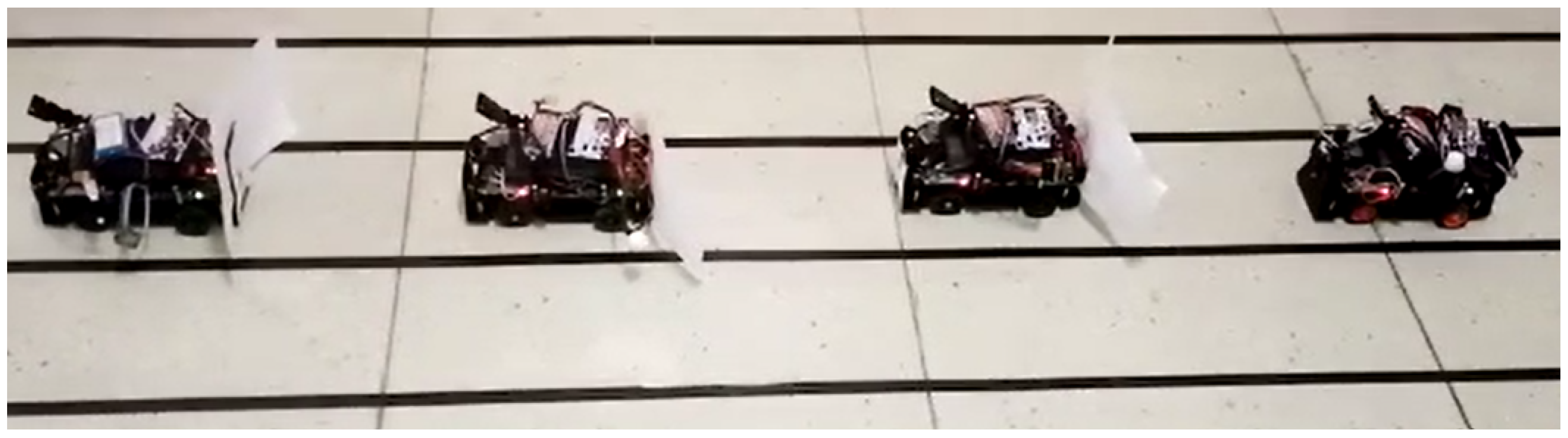
In this work, a four-vehicle platoon is used, composed of four mobile robots, as depicted in
Figure 1.
The mobile robots have a distributed architecture consisting of a dsPIC-based main board, an ESP8266-based board used for V2V communication, and a Raspberry PI, which together with a camera, acts as a machine vision system. The three computing systems communicate with each other via UART serial communication channels. The MPLAB IDE environment was used for easy development and debugging of the dsPIC software application.
The longitudinal control is based on the information provided by an analog infrared distance sensor. The sensor is connected to the dsPIC and is located at the front of the vehicle. Each mobile robot was designed to be car-like. Moreover, the steering acts upon the front wheels, whilst the drive motor is placed in the back. The steering respects the Ackermann steering geometry and is it driven by a servomotor. Each mobile robot is powered by 2 cells Li-Ion rechargeable battery, while an external battery is employed for powering the Raspberry PI module. The dsPIC application can save all the required data in specific local log files by means of a micro-SD card module.
The DC motor is equipped with a magnetic quadrature encoder able to generate 12 pulses per rotation. From the dsPIC, a dedicated quadrature encoder interface and a timer were used to determine the mobile robot’s travel velocity, based on the quadrature signals provided by the encoder. The minimum sampling frequency was calculated to correctly implement the velocity computing method. Based on the maximum motor velocity and according to the Nyquist–Shannon theorem [
22], it was determined as approximately 10 Hz; therefore, the real-time counter was configured to generate periodic interrupts at 0.1 s. The velocity was computed on the interrupt service routine level, the method assuming interpolation of the counter register corresponding to the interface monitoring the encoder output into an angular position.
3.2. Identification Procedure of the Mobile Robots
The mathematical model for each mobile robot was computed from experimental data obtained via an open-loop identification procedure. To this end, for each mobile robot, an excitation signal was designed, as a series of three rectangular pulses with approximately the same width of 20 s and different amplitudes (i.e., 20,000, 26,000, and 30,000). This 16-bit signal represented as an unsigned binary signal in the range 0 through 65,535 was sent as an input signal, and was written into the PWM’s duty cycle control register assigned to the DC rear servomotor of the mobile robot. The output signal recorded from each mobile robot for the identification procedure purpose is the velocity of the mobile robot, measured in cm/s. In
Figure 2, the identification signals for the open-loop experiment are represented. For simplicity, only the identification signals used for the first mobile robot from the platoon (denoted
) are depicted.
The mathematical model for each mobile robot was obtained using the System Identification Toolbox available in Matlab 2021a. Since the purpose was to thoroughly investigate the mobile robot’s dynamics, the identification data were split into the corresponding three ranges, which were used to identify the matching model. For each mobile robot, the largest best-fit value was obtained for the second data set (i.e., the input of amplitude 26,000 units and the velocity of 20 cm/s). The validation of the model for the first platoon vehicle, for the second data set was successfully established with a best fit of
. In
Figure 3, the fit between the measured data and the simulated model for the input amplitude of 26,000 units and the velocity of 20 cm/s is depicted.
The identified first-order, transfer function model obtained for the first mobile robot from the platoon (i.e.,
) is given in (
9):
where
is the gain, and
is the time constant of the first-order transfer function.
Moreover, following the same identification procedure (using identical identification signals) for the remaining three mobile robots, the following first-order transfer function models were obtained:
The validation of
,
, and
was performed with a best fit of
,
, and
, respectively. The open-loop step response corresponding to models
,
, obtained for an input signal of amplitude 26,000 units is given in
Figure 4. As expected, the simulation results show that all mobile robots have different dynamics, obtaining a heterogeneous vehicle platoon. The platoon was configured with the fastest vehicle in the leading position (i.e.,
modeled by
), toward the slowest of the remaining vehicles, with a quasi-identical response (i.e.,
and
, modeled by
and
, respectively).
Since the CC methodology is designed using the state-space formulation, starting from the continuous-time transfer functions (
9) and (
10), the following state-space model is obtained:
where the state vector
,
contains the distance error
, the velocity
and the integral of the distance error
; the control input for the rear servomotor
is represented as an unsigned binary signal, whereas the controlled output
is the distance error
;
The distance error
is computed as the difference between inter-vehicle distance
, where
denotes the position of vehicle
i, and
denotes the imposed headway reference, which in this work is assumed constant. It results that, the derivative state of the distance error
, can be computed based on the velocity difference between two consecutive vehicles. To this end, according to (
11), for simulation purposes, each follower vehicle must receive only the velocity of the vehicle in front of it (i.e., the coupling signal
).
The first vehicle in the platoon does not have a vehicle in front of it and, thus, does not receive a coupling signal . In this case, it is considered that there exists a ‘virtual vehicle’ in front of the platoon leader, which imposes a reference velocity value for the entire platoon. Thus, the platoon leader will travel with a velocity imposed by the ‘virtual leader’.
4. Results and Discussion
In this section, the coalitional control results achieved in the vehicle platooning application are presented. Two communication topologies were tested in both simulation and laboratory experiments, with the following feedback gain matrices:
The decentralized (DEC) topology, with no communication links enabled between vehicles:
with
a zero matrix with adequate dimensions and
The leader–following (LF) topology—with communication links enabled between the leader vehicle and all follower vehicles:
with
,
given in (
13) and
The optimal state feedback gain matrix
K for the decentralized topology was computed by solving the optimization problem (
2)–(
4), with the following optimization parameters: the sampling period
s, the simulation time length
s, the state weight matrices
,
, the input weight factor
and
. The control input limits are
and
, corresponding to the 16-bit binary representation of the signal. The maximum value of
, which ensures the closed-loop stability for the decentralized topology.
The optimal state feedback gain matrix
K for the leader–following topology was computed by solving the optimization problem (
5)–(
8), using the same optimization parameters values, as the ones used in (
2). In addition, the tracking error weight parameter is chosen
,
, which emphasizes the interest given to solving the tracking problem when compared with the size of input increment and state value. The maximum value of
, which ensures the closed-loop stability for the leader–following topology. All values for the optimization parameters were selected empirically, to obtain the best simulation results.
The set
contains 25 desired reference trajectories with a length of 60 s, each one designed as a step change at a time of 30 s, from an initial value to a final value. The initial and final values for the step amplitudes were randomly selected in the range
cm/s, and
cm/s, respectively. These values were selected considering that each mobile robot model was identified in the operation point around 20 cm/s. The desired reference trajectory profiles are provided in
Figure 5.
Each communication topology was tested in both simulation and laboratory conditions, in a reference tracking experiment, designed as follows:
The leader vehicle follows a velocity trajectory imposed by the ‘virtual leader’ of the platoon, described as a series of step changes of amplitude: 0 cm/s for time interval s, 8 cm/s for time interval s and 15 cm/s for time interval s.
The follower vehicles follow a constant imposed inter-vehicle distance reference trajectory 30 cm.
4.1. Simulation Results
In this section, the simulation results for a vehicle platooning application with four vehicles are provided. For simulation purposes, Algorithms 3 and 4 were implemented, for the decentralized and leader–following topology, respectively.
| Algorithm 3: DEC communication topology |
| Initialization phase—compute the optimal state feedback gain matrix K, by |
| minimizing the cost function (2). |
| For
|
| Each vehicle i |
| 1. Prepares the state information, which will be used in the simulation by the |
| following vehicle , in step 3, i.e., the current velocity state is saved. |
| 2. Computes the control law using the corresponding values from the optimal |
| state feedback gain matrix, i.e., the control law is calculated using (4). |
| 3. Updates the state vector by simulating the vehicle model (11). |
| 4. Saves the updated state vector. |
| end |
In Algorithm 3,
M denotes the length of the simulation, and
k denotes the sampling time index. As was previously mentioned, in step 3, the leader vehicle
uses the current value from the velocity reference trajectory
imposed by the ‘virtual leader’ of the platoon. This value is used in (
11), instead of the velocity variable
. Moreover, in step 2 of the algorithm, for each vehicle, the optimal state feedback gain matrix is assumed known, since it was computed in the initialization phase of the algorithm.
| Algorithm 4: LF communication topology |
| Initialization phase—compute the optimal state feedback gain matrix K by |
| minimizing the cost function (5). |
| For
|
| Each vehicle i |
| 1. Prepares the state information, which will be used in the simulation by the |
| following vehicle , in step 3, i.e., the current velocity state is saved. |
| 2. Computes the control law using the corresponding values from the optimal |
| state feedback gain matrix, i.e., the control law is calculated using (8). |
| 3. Updates the state vector by simulating the vehicle model (11). |
| 4. Saves the updated state vector. |
| end |
It is noteworthy to mention that in step 2 of Algorithm 4, the follower vehicles compute the control action using (
8) and the state vector prepared by the leader vehicle, whereas, the leader vehicle, computes its control action using (
4). For the simulation of the platoon, in step 3, the follower vehicles use only the velocity state from the vector prepared by the preceding vehicle in step 1.
In
Figure 6, the results obtained for the CC methodology with decentralized topology are provided, for one of the velocity reference profiles from
Figure 5. The upper plot depicts the leader’s velocity, the middle plot depicts the headway for the follower vehicles, and the lower plot depicts the control effort for all vehicles. The CC results for the LF topology are given in
Figure 7, in an identical manner.
In order to evaluate the performances obtained in simulation for the proposed communication topologies, a qualitative assessment in terms of both the mean squared error (MSE) and arithmetic mean (MEAN) index is given. The MSE index was computed for each vehicle from the platoon,
, where
and
,
are the values for the imposed reference and the controlled output, respectively.
M is the length of the simulation, in our case 40 s. For the leader vehicle, the
index was computed with respect to the velocity error, whereas for the follower vehicles, the index was computed with respect to the headway error. The MEAN index was computed for all vehicles
for the control input value, which is positive (
). In
Table 1, both indices for both topologies are provided.
When analyzing the performance indices, it results that the LF topology has a decrease in the MSE index, indicating better tracking performance, than the decentralized topology. The MEAN index shows that the control effort for both topologies remains unchanged, even if additional communication links are enabled. This is mainly caused by the magnitude difference between the values from the main diagonal and the first column from the optimal state feedback gain matrix
K given in (
15).
4.2. Experimental Results
In this section, the experimental results for a vehicle platooning application with four mobile robots are provided. In the real-time experiments, Algorithm 5 was implemented for the decentralized topology, whereas Algorithm 6 was implemented for the leader–following topology.
In Algorithm 5, for time instant , the distance error and the integral of the distance error state values, where are initialized to 0 since no measurements are yet performed. In order to implement Algorithm 5 on the platoon vehicles, for the leader vehicle, only steps 1–6 are performed, while for the follower vehicles, only steps 7–13 are used. Moreover, depending on the two categories, the corresponding reference trajectories and feedback gain matrices are selected. Furthermore, all the computations performed on a mobile robot must be finished within a sampling period .
Remark 3. In this work, in the experimental tests performed on the platoon of mobile robots, only the input and output trajectories were saved, i.e., for the leader vehicle ( and variables), whereas for the follower vehicles ( and , variables), at steps 5 and 11, respectively. This was caused by the limitations in the storage capacity of the mobile robots, together with the additional computational steps performed to save the relevant information at each sampling period.
It is noteworthy to mention that in Algorithm 6, there is one additional step to be performed by each mobile robot, i.e., in Step 5, the leader broadcasts its current state variables to all the platoon followers, while in Step 12, the followers receive the state vector from the leader, via the communication network. This means that all the mobile robots must be synchronized, i.e., the transmission and reception operations must be performed in the same sampling period.
The platoon is implemented in real-time, using the dsPIC embedded application, which is based on the real-time operating system FreeRTOS. This operating system allows the easy development of application tasks, which can be synchronized and able to communicate by means of FreeRTOS-provided mechanisms.
The velocity control is implemented as an aperiodic task, synchronized with the velocity computation via a binary semaphore. The velocity control task computes the command as a 16-bit unsigned integer. The value obtained by applying the control law is written into the PWM’s duty cycle control register assigned to the DC motor.
| Algorithm 5: DEC communication topology-based implementation |
| Initialization phase—compute the optimal state feedback gain matrix K, by |
| minimizing the cost function (2). |
| For
|
| The leader vehicle |
| 1. Measures the current velocity using the onboard sensors. |
| 2. Computes the distance error state using the velocity measured at step 1 |
| as follows:
3. Updates the integral of the distance error state as follows: |
|
4. Computes the control law using the corresponding values from the optimal |
| state feedback gain matrix, i.e., the control law is calculated using (4) as follows:
5. Applies the command to the DC motor. |
| 6. Saves the state and input variables. |
|
Each follower vehicle |
| 7. Measures the current velocity using the onboard sensors. |
| 8. Measures the current inter-vehicle distance with respect to the vehicle |
| in front of it using the onboard sensors. |
| 9. Computes the distance error state using the inter-vehicle distance measured |
| at step 8 as follows:
10. Updates the integral of the distance error state as follows:
11. Computes the control law using the corresponding values from the optimal |
| state feedback gain matrix, i.e., the control law is calculated using (4) as follows:
12. Applies the command to the DC motor. |
| 13. Saves the state and input variables. |
| end |
For the CC with leader–following communication topology, for the leader vehicle, in the velocity control task, an additional step is included, i.e., to prepare the message to be broadcast to the whole platoon. To this end, a string with a total length of 9 bytes is constructed. Before the message is constructed, the velocity together with the distance error and the integral of the distance error are multiplied by a factor of ×1000 for better resolution at reception. The three system states are stored in pairs of 2 bytes located next to each other. At the same time in case of negative values, the byte reserved for the sign is set to 0xFF, the nominal value being 0x01—for positive values. The message stored in the transmission buffer is sent to the ESP8266 via the UART port. Once the message is received at the ESP8266 level, the content is broadcast to the whole platoon.
| Algorithm 6: LF communication topology-based implementation |
| Initialization phase—compute the optimal state feedback gain matrix K, |
| by minimizing the cost function (5). |
| For
|
| The leader vehicle |
| 1. Measures the current velocity using the onboard sensors. |
| 2. Computes the distance error state using the velocity measured at step 1 |
| as follows:
3. Updates the integral of the distance error state as follows:
4. Computes the control law using the corresponding values from the optimal |
| state feedback gain matrix, i.e., the control law is calculated using (8) as follows: |
|
5. Broadcasts the state vector to all platoon followers. |
| 6. Applies the command to the DC motor. |
| 7. Saves the state and input variables. |
| Each follower vehicle |
| 8. Measures the current velocity using the onboard sensors. |
| 9. Measures the current inter-vehicle distance with respect to the vehicle |
| in front of it using the onboard sensors. |
| 10. Computes the distance error state using the inter-vehicle distance |
| measured at step 8 as follows:
11. Updates the integral of the distance error state as follows:
12. Receives the state vector from the leader vehicle. |
| 13. Computes the control law using the corresponding values from the optimal |
| state feedback gain matrix, i.e., the control law is calculated using (8) as follows:
14. Applies the command to the DC motor. |
| 15. Saves the state and input variables. |
| end |
Further on, follower vehicles from the platoon will transmit to their corresponding dsPIC, the message received from the leader vehicle. For the follower vehicles, once the dsPIC receives the message transmitted from the leader, the aperiodic longitudinal control task computes the command for the traction DC motor, based on local and received information. In this manner, the task’s period is ensured by the leader vehicle’s transmissions. The control command, as in the case of the vehicle control task, represents the duty cycle of the PWM signal used to drive the DC motor.
In
Figure 8, the results obtained for the CC methodology with decentralized topology are provided. The upper plot depicts the leader’s velocity, the middle plot depicts the headway for the follower vehicles, whereas the lower plot depicts the control effort for all vehicles. The CC results for the LF topology are given in
Figure 9, in an identical manner.
In
Table 2, the MSE and MEAN performance indices for the decentralized and leader–following communication topologies are provided.
The experimental results show a major difference between the two communication topologies, which can be also noted in the performance indices. The LF topology outperforms the decentralized topology without enabled communication links, in terms of MSE and MEAN indices. However, we note that both communication topologies have similar control efforts, despite the reference tracking differences.
4.3. Discussion
In the experimental tests performed using the mobile robots, when the LF communication topology was used, the communication network was used to broadcast the leader’s state vector to the platoon followers. This was the only information disseminated in the network, at each sampling time, and was used to compute the LF control law for the follower vehicles.
The DEC and LF communication topologies tested in this work are the initial step in developing a CC methodology, as previously described. This work is a proof of concept that the vehicle platoon composed of mobile robots can be controlled using the two proposed communication topologies, which at this time were tested independently.
Furthermore, in order to develop a CC methodology, one must introduce a switching criterion, which will be used to transition between the two available topologies. Since the real-time results for the DEC topology show larger values for the MSE error, with respect to the inter-vehicle distance reference, suitable switching criteria for our mobile robots platoon, can be obtained with a threshold value for the tracking error for the followers. This means that after the transient response (around 10 s into the experiment), when the tracking error is above the threshold, for at least one follower, the communication topology will switch to LF communication, for that particular platoon follower. This CC strategy could possibly improve the reference tracking performance for vehicle
, in the time interval [20 … 30] s (see
Figure 8). This is because, additional information (i.e., the leader’s state vector in our case) is used only when needed. Moreover, the CC methodology would return automatically to the
communication topology, when the tracking error decreases below the threshold value. If this is the case, both the
matrix and the leader’s state vector must be available, in order to compute the LF control low. In a CC strategy, in the initialization phase of the algorithm, all vehicles would receive access to both
K matrices, corresponding to each communication topology.
A more complex CC methodology will involve the switching between multiple communication topologies. Nevertheless, the platoon starts from the decentralized topology, and activates communication links between different platoon members, depending on the switching criteria. For a vehicle platooning application, with uni-directional communication flow, there are a finite number of communication topologies, determined by the platoon size (e.g., a coalition between vehicles , or ). Also, there are some combinations that are not eligible, for example, a coalition between , without vehicle acting as an intermediary. To implement this CC methodology, an intermediate development stage is to separately test all eligible communication topologies and to assess their efficiency and performance. Since the CC methodology takes advantage of the benefits of different communication topologies within a single experiment, one must first evaluate if some combinations must be avoided, by evaluating beforehand what are their standalone performances.
Remark 4. Both simulation and experimental results suggest that an optimal state feedback gain matrix can be used in a vehicle platooning application. The control strategy is easy to implement on embedded systems, since the control action is computed by scalar multiplication, between the measured or received system variables and the feedback gain values. The challenging part of the design is shifted to the offline initialization part of the algorithm when the state feedback gain matrix is computed. After the control matrix K is calculated by solving an optimization problem, it can be deployed on the embedded system and used in real-time experiments.


 ,
, 


