Algorithmic Approach for a Unique Definition of the Next-Generation Matrix

Abstract

The basic reproduction number $R_0$ is a concept which originated in population dynamics, mathematical epidemiology, and ecology and is closely related to the mean number of children in branching processes (reflecting the fact that the phenomena of interest are well approximated via branching processes, at their inception). Despite the very extensive literature around $R_0$ for deterministic epidemic models, we believe there are still aspects which are not fully understood. Foremost is the fact that $R_0$ is not a function of the original ODE model, unless we also include in it a certain $(F,V)$ gradient decomposition, which is not unique. This is related to the specification of the “infected compartments”, which is also not unique. A second interesting question is whether the extinction probabilities of the natural continuous time Markovian chain approximation of an ODE model around boundary points (disease-free equilibrium and invasion points) are also related to the $(F,V)$ gradient decomposition. We offer below several new contributions to the literature: (1) A universal algorithmic definition of a $(F,V)$ gradient decomposition (and hence of the resulting $R_0$). (2) A fixed point equation for the extinction probabilities of a stochastic model associated to a deterministic ODE model, which may be expressed in terms of the $(F,V)$ decomposition. Last but not least, we offer Mathematica scripts and implement them for a large variety of examples, which illustrate that our recipe offers always reasonable results, but that sometimes other reasonable $(F,V)$ decompositions are available as well.

1. Introduction

Motivation. Mathematical epidemiology had started by proposing simple models for specific epidemics and computing explicitly certain important characteristics like the basic reproduction number and the final size; for example, the SIR model was introduced, among other concepts, in the celebrated “A contribution to the mathematical theory of epidemics” [1]. The most fundamental, and actually the only general result of the field due to Diekmann, Heesterbeek, Van den Driesche and Watmough, expresses the disease-free equilibrium stability domain in terms of $R_0$, which is defined as the Perron–Frobenius eigenvalue of a certain $(F,V)$ gradient decomposition (this is presented in detail in Section 2.2). But, since the $(F,V)$ decomposition is not unique, it seems to us that the question of what $R_0$ is still deserves further discussion.

On the other hand, one may note that nowadays, mathematical epidemiologists typically either restrict themselves to low-dimensional models, resolved symbolically, even by hand, or consider very complicated models which are resolved only numerically, for particular values gleaned from the medical literature. Missing from here are moderately complex models, which may be solved partly symbolically for any values of the parameters, but in a way where the use of computer algebra systems (CAS) is either indispensable or greatly facilitating. Even in the case of papers belonging to this level—see, for example [2], that the role of the CAS is deemphasized. Our paper is also an attempt to cast the CAS as one of the main heroes of our story.

Our main result. We provide below, for the first time, a universal recipe for choosing a natural $(F,V)$ gradient decomposition, which only requires specifying the disease compartments (a subset of those which are zero for the boundary point under consideration) (informally, these are not far conceptually from the so-called fast components of singular perturbation theory). This decomposition is useful both for determining $R_0$ and for computing the extinction probabilities of an associated stochastic model. We identify also examples in which the $(F,V)$ decomposition is not unique and in which choosing another decomposition with F of a lower rank may be beneficial for simplifying the $R_0$ formula.

First restriction (among others to follow). In this paper, we will restrict to mathematical epidemiology models for which there exist at least two possible special fixed states. The first, the disease-free equilibrium (DFE), corresponds to the elimination of all possible compartments involving sickness and will be assumed to be unique. Typically, this point is locally stable only for certain values of the parameters. Outside of this domain, it is typically replaced by another fixed point, which will be called “endemic“ if all its components are positive, and ”resident boundary point” otherwise.

Importantly, the stability of the DFE may be related to the historically famous basic reproduction number and net reproduction rate—see (1). These pillar concepts in population dynamics, mathematical epidemiology, virology, ecology, etc., were already introduced by the father of mathematical demography Lotka—see [3,4]—and also the introduction of the book [5], and in [6], the authors described the stability of the solution of differential systems.

A bit of history of the net reproduction rate $\mathcal{R}$, and its evolution into the mathematical concept of basic reproduction number/stability threshold $R_0$. Loosely speaking, in the case of only one infectious class, the net reproduction rate $\mathcal{R}$ describes the expected number of secondary cases which one infected case would produce in a homogeneous, completely susceptible population during the lifetime of the infection. This description is especially relevant at the start of an epidemic, when the dynamics is well approximated by that of a branching process (a fact which goes back to Bartlett and Kendall—see for example [7,8]). The main characteristic of a branching process is the “fertility”, i.e., the expected number of descendants one individual produces in the next generation. As a consequence, in epidemiology, the branching result insuring extinction when the fertility is less than one translates into local stability results of the disease-free equilibrium involving $\mathcal{R}$.

The reproduction number $\mathcal{R}$ intervened already, in a particular case, in the foundational paper “A contribution to the mathematical theory of epidemics” [1], which showed that:

1.

The condition

$$R_0<1,\mathrm{where}{R}_0={\mathsf{s}}_{dfe}\mathcal{R},$$

(1)

implies local stability of the DFE. Here $\mathcal{R}$ is the net reproduction rate (number of secondary infections produced by one infectious individual), and ${\mathsf{s}}_{dfe}$ is the fraction of susceptibles at the DFE.

2.

The condition

$$R_0>1$$

implies instability of the DFE.

With more infectious classes, one deals, at the inception of an epidemic, with approximate multi-class branching processes, whose stability is determined via a “next-generation matrix” (NGM)—see Section 2.2.

The “Jacobian approach” for computing $R_0$. For big size problems, this approach is doomed to fail symbolically, since it is equivalent to the Routh–Hurwitz conditions (RH), which rarely succeed symbolically beyond dimension 4 (also, RH is irrelevant numerically, since the eigenvalues themselves are just as easy to compute). Therefore, we studied below a variant, the “Jacobian factorization approach”, which focuses on an approximation, which we show to yield always upper or lower bounds of the NGM $R_0$, depending on whether $R_0\le 1$ or not—see Theorem 1. Several questions around this bound are scattered below in Section 6.3, Section 8.1, and Section 8.2.

Note, as mentioned in [9], that an example where the Jacobian method does not yield $R_0$ is offered in [10] (Exe 5.43) and that of [11] suggesting that when threshold parameters determined from the Jacobian do not have the biological interpretation of the dominant eigenvalue of the next-generation matrix, then they should not be called basic reproductive ratios nor denoted as $R_0$ (we follow their suggestion and use the notation $R_J$ in this case).

The dilemma of the several different methods for computing $R_0$ has been discussed in many papers, see for example [9,12]. But, this is a direct consequence of the non-uniqueness of the $(F,V)$ decomposition.

Deterministic or stochastic models? Most of the mathematical epidemiology papers belong exclusively to one of these two paradigms. However, any deterministic model may also be viewed as a stochastic continuous time Markov field (CTMC) evolving on the integers. One interesting CTMC, which seems not to have been discussed before, is presented in Section 2.4.

Contents. Our paper is structured as follows. Section 2 recalls the definition of the DFE and provides our algorithmic definition of the (F, V) decomposition, in the form of a Mathematica script, as well as a discussion—see Remark 6—of why other decompositions might turn out useful. This section also provides a new Equation (8) for computing extinction probabilities for associated continuous time Markov chain models in terms of the $(F,V)$ decomposition, showing that the Jacobian factorization approach yields upper bounds and lower bounds for NGM $R_0$’s in Appendix A.

We turn then to a series of examples, chosen to help investigate what may be the major open problem in the field nowadays, which, in our opinion, relates on one hand to $R_0$, and on the other hand, to the extinction probabilities—see below—and duration of minor epidemics [13,14,15,16,17], which is not further touched on here.

Let us now briefly explain why so many examples were included in the paper.

Section 4 is dedicated to a host-only model, with a single susceptible class and an F matrix of rank one, where the formula of $R_0$ may be “guessed by inspection” of the flow chart. These kinds of examples have kept alive the hope of “interpretable $R_0$ formulas”, as illustrated in other recent papers—see for example [18,19]. But in fact, as far as we know, no interpretable $R_0$ formula has emerged outside the rank one case, which is already fully studied in [20]. The papers [18,19] start by presenting simple rank one cases, then proposing algorithms for more complex cases based on the graph structure of the flow chart, which, in our opinion, are not sufficiently detailed or documented. While it may well be that tools like Petri nets, as proposed in the second paper, will one day succeed for resolving flow charts with certain structures, this does not seem to have happened yet. Also, for models with a next-generation matrix of high rank, the lack of simple formulas for $R_0$ and of “simple biological interpretations” is naturally to be expected; simple formulas for the spectral radius can only be a consequence of a simple graph structure which has not been pinpointed yet.

Section 5.1 and Section 7.1 offer two examples in which several $R_0$ formulas were offered in the literature, but we are at a loss of how to choose among them. In the first case (a virus–tumor model), the recipe $R_0$ is simpler than its competitor, but in the second case (a vector–host model), it is more complicated.

Section 6.2 shows that the boundary equilibria and the (invasion) reproduction numbers may be easily computed with our scripts; to illustrate this, we use a two-strain host-only model from [21] (Ch.8), where our recipe NGM yields the same answer as that given by the Jacobian factorization.

Section 6.3 offers another two-strain host-only example, this time including also vaccination, in which our recipe NGM yields again the same answer as that given by the Jacobian factorization.

Section 7.2 offers an example from the textbook of [21] in which the square relation stops holding.

Section 8.1 and Section 8.2 offer yet more examples, this time in the two-strain vector–host context, in which our recipe NGM yields an $R_0$ formula which is precisely the square root of that given by the Jacobian approach. Note that here, the first of the three elegant relations concerning the invasion numbers from Section 6.3—see Remark 22—holds, but the other two seem to break down.

The last subsection provides, for the invasion numbers, a second example where another choice of $R_0$ may be more reasonable, on the grounds of leading to a simpler answer (but the admissibility requirement forces then extra assumptions on the parameters).

2. A Bird’s Eye View of Mathematical Epidemiology: The Disease-Free Equilibrium, the Next-Generation Matrix, and an Algorithmic Definition of a Stability Threshold Associated to the Basic Reproduction Number ${\mathit{R}}_{\mathbf{0}}$

2.1. The Disease-Free Equilibrium (DFE)

The DFE may be defined as a “maximal boundary state” and may be found by identifying a maximal sub-system of the ODE epidemic model which factors

$${\mathit{i}}^{\prime }=M\mathit{i},$$

(2)

where the prime denotes the derivative with respect to time, and M is a matrix that may depend on $\mathit{i},$ but also may not explode in the domain of interest, which we will take for the sake of simplicity to be ${\mathbb{R}}_{+}^n$.

Remark 1. 

One fixed point of this system is $\mathit{i}=0$. This motivates us to call the components $\mathit{i}$ disease or infectious states. The set of all its indices will be denoted by $\mathcal{I}$. Note that specifying ‘$\mathcal{I}$ induces a partition of both the coordinates and the equations of our original system into infection (eliminable) and “non-infection” (the others) components.

The eventual other fixed points may be found by solving $M=0$ together with the other non-infection equations under the condition $\mathit{i}=0$.

In this paper, we will assume the uniqueness of the DFE, at least after excluding biologically irrelevant fixed points, like an unreachable origin.

We end this section with the very elementary script that implements this. Note that any ODE model “mod” (like SIR, etc…) is a pair mod = (dyn,X) consisting of a vector field “dyn” and a list of variables “X”, and that to find any boundary fixed point, it suffices to know the set of indices “inf” where it is 0, so that we solve the system “dyn==0” under the condition “X[[inf]]->0”. But, since sometimes only numeric solutions are possible, our DFE Mathematica script below also has an optional numerical condition parameter “cn”, which is taken by default as the empty set.

 

 DFE[mod_,inf_,cn_:{}]:=Module[{dyn,X},

  dyn=mod[[1]]/.cn;X=mod[[2]];

  Solve[Thread[dyn==0]/.Thread[X[[inf]]->0],X]];

 

For the non-Mathematica users, only the Solve command is relevant, with the others being just Mathematica implementation details.

2.2. $(F,V)$ Gradient Decompositions, the Next-Generation Matrix, $R_0$, and a Simple Recipe for Computing Them

From now on, the infection Equation (2) will be rewritten as

$${\mathit{i}}^{\prime }=\mathcal{F}-\mathcal{V}=(F-V)\mathit{i}.$$

(3)

Of course, such a decomposition is not unique, but we will also ask, following [7,22,23], that F, the gradient of $\mathcal{F}$, is a matrix with non-negative elements, and $-V$, the gradient of $-\mathcal{V}$, is a Markovian generating matrix (i.e., a matrix with non-negative off-diagonal elements and non-positive row sums). Conceptually, F models input to the disease compartments from outside (”new infections”), and $-V$ models transfer between the disease compartments. Still, a priori, the decomposition (3) is not unique.

Example 1. 

Let us illustrate this via an SIR example with superinfection parameter ξ, in which the classes S and R play symmetric roles inspired by the works of [24,25,26]

$$\begin{array}{c}\hfill \left\{\begin{array}{cc}{\mathsf{s}}^{\prime }\left(t\right)\hfill & ={\Lambda }_s-\mathsf{s}\left(t\right)\left[{\beta }_s\mathsf{i}\left(t\right)(1+\xi \mathsf{i}\left(t\right))+d_s\right]+i_s\mathsf{i}\left(t\right)+{\gamma }_r\mathsf{r}\left(t\right)\hfill \\ {\mathsf{i}}^{\prime }\left(t\right)\hfill & =\mathsf{i}\left(t\right)\left[\left[{\beta }_s\mathsf{s}\left(t\right)+{\beta }_r\mathsf{r}\left(t\right)\right](1+\xi \mathsf{i}\left(t\right))\right]-d_i\mathsf{i}\left(t\right),d_i=i_r+i_s+{\Lambda }_s+{\Lambda }_r+\delta \hfill \\ {\mathsf{r}}^{\prime }\left(t\right)\hfill & ={\Lambda }_r-\mathsf{r}\left(t\right)\left[{\beta }_r\mathsf{i}\left(t\right)(1+\xi \mathsf{i}\left(t\right))+d_r\right]+i_r\mathsf{i}\left(t\right)+{\gamma }_s\mathsf{s}\left(t\right)\hfill \end{array}\right..\end{array}$$

When $\xi =0,$ this reduces to the symmetric SIR model introduced for mathematical purposes by [25,26], in which births may also directly enter the R class, with parameter ${\Lambda }_r$, and may also infect, with parameter ${\beta }_r$. Furthermore, there are linear flows from $\mathsf{i}$ to both $\mathsf{s}$ and $\mathsf{r}$, where the former does not make epidemiologic sense.

Here, the only infection equation, the second, is already written in a decomposed form $\mathcal{F}-\mathcal{V},\mathcal{V}=d_i\mathsf{i}\left(t\right)$, and $F=\left[\left[{\beta }_s\mathsf{s}\left(t\right)+{\beta }_r\mathsf{r}\left(t\right)\right](1+\xi \mathsf{i}\left(t\right))\right]+\xi \mathsf{i}\left(t\right)\left[{\beta }_s\mathsf{s}\left(t\right)+{\beta }_r\mathsf{r}\left(t\right)\right]$.

Note that for the application of the next-generation matrix method, we must finally plug $\mathsf{i}=0$; therefore, the second term in F, due to ”superinfection”, is irrelevant for this purpose.

Remark 2. 

The possible non-uniqueness of the decomposition brings us to a delicate point in mathematical epidemiology. Anticipating a bit, since $R_0$ is the Perron–Frobenius eigenvalue of $F{V}^{-1},$ strictly speaking, $R_0$ is not determined just by an ODE epidemical model, but also by the $(F,V)$ gradient decomposition. If we want an ODE epidemical model to uniquely determine an $R_0$, we must include, in the definition of the ODE epidemical model, the $(F,V)$ gradient decomposition we also adopt.

Remark 3. 

For us, an ODE epidemic model is an ODE dynamical model in which a certain subset of equations, usually called “disease/infection” equations, referred from now on as a zeroable set, admits at least one admissible decomposition (3), with $(\mathcal{F},\mathcal{V})$ satisfying the conditions (A1–A5) of [23].

Remark 4. 

Note that (3) is the most common model used in population dynamics. This makes it natural to informally define ODE epidemic models as population dynamics models (3), with extra equations modeling interactions with the non-disease compartments, which admits at least one admissible decomposition.

Remark 5. 

The definition of ODE epidemic models above is imprecise, since it does not list all the requirements we must put on an ODE model. Some reasonable restrictions are

1. 

Essentially non-negative processes have a non-empty set of disease classes, so we deal with an epidemic (note, however, that we define disease classes in the sense of classes which satisfy (2), which excludes, for example, importation models).

2. 

Processes with a unique DFE, at least after excluding biologically irrelevant fixed points, like an unreachable origin.

3. 

The local stability domain of the DFE is non-empty and not the full set.

4. 

The dynamical system has polynomial coefficients to be able to take advantage of the remarkable symbolic computation tools available for this class.

We make these assumptions because they are satisfied by most mathematical models which have already been used for modeling real-life biological phenomena. However, these assumptions might not be enough and further ones might be necessary for obtaining the currently missing precise definition of “real life ODE mathematical epidemiology models”.

Remark 6. 

Admissible decompositions need not be unique. A priori, one may “move terms from F to V”, to lower its rank and simplify the formula for $R_0$, and also “move off-diagonal terms from V to F”, which enlarges the domain of parameters which ensure that $V^{-1}$ has positive terms. There is a tradeoff between these two possible moves, since the simplicity of $R_0$ comes at the cost of extra assumptions on the parameters. Our universal decomposition seems to strike a balance between the two directions.

Remark 7. 

It was emphasized from the outstart—see for example [12,27,28,29]—that an ODE mathematical epidemiology model might have several “admissible decompositions”, which might yield distinct next-generation matrices and distinct $R_0$’s.

For any admissible decomposition, Diekmann, Heesterbeek, Van den Driesche, and Watmough established the following celebrated DFE stability theorem:

Proposition 1. 

For any admissible decomposition $(F,V)$, let

$$R_0=\rho \left(F{V}^{-1}\right)$$

denote the Perron–Frobenius eigenvalue of the next-generation matrix. Then, the DFE is unstable on $R_0>1,$ and locally stable on $R_0<1$ [7,10,22,23].

For a recent historical overview of $R_0$, next-generation matrices, and their calculation in many examples, we refer the reader to the delightful paper [30].

Unfortunately, the standard definition of a next-generation matrix (and hence of $R_0$) involves concepts like “new infections”, which were defined in the original papers based on epidemiological considerations and therefore require the intervention of a human expert. This had created the impression that this method cannot be encapsulated into a computer program. However, we offer and implement below a simple algorithmic definition, based only on the structure of the system and of the “infectious/disease equations”.

Our proposal is to use a special F-V decomposition, with F constructed as the positive part of all the interactions in the disease equations which involve both disease compartments and input/susceptible ones. The latter are defined as the complement of the disease compartments, after the possible removal of output compartments, which may be specified as deterministic functions of the other compartments (i.e., may be computed, once the other compartments are known). Note now that the concept of the “positive part of the interactions” may be hard to pinpoint mathematically, but useful enough to have been implemented in CAS’s (Mathematica, Maple, Sage, etc.); this made us adopt the following definition:

Remark 8. 

For a given zeroable set, an admissible $(F,V)$ gradient decomposition (3) is one where F, the gradient of $\mathcal{F}$, does not contain, in its expanded form, syntactic minuses in its CAS representation, and also where V, the gradient of $\mathcal{V}$, is such that $-V$ is a “sub-generating matrix” under the assumption of non-negativity of all the model parameters.

The problem of whether the $R_0$ of the decomposition provided satisfies, under certain conditions, the stability theorem of Van den Driessche and Watmough is still open; therefore, it should be viewed for now just as a recipe that works well in simple cases.

After lots of experimenting, we have found only few cases—see for example Section 8.2, where the recipe NGM has a serious competitor; it is for computing the invasion reproduction number for a two-strain vector–host model, with altered infectivity for co-infected vectors, and with ADE (antibody-dependent enhancement).

2.3. An Algorithmic $F-V$ Decomposition

We complement now the famous $\mathcal{F}-\mathcal{V}$ “equations decomposition” and the next-generation matrix method of [7,22,23] using a algorithmic $F-V$ decomposition.

1.

The user supplies the model “mod” (a pair containing the RHS of the dynamical system and its variables) and the indices “inf” of the disease (or infectious) variables; the indices of the other compartments are denoted by “infc”.

2.

Subsequently, the Jacobian of the infectious equations M with respect to the corresponding variables is computed.

3.

Define the interaction terms as terms in M which contain variables $s\in \mathrm{infc}$, and which, if positive, must end up in F. Their complement, denoted by $V1$, will form part of V.

4.

As a first guess for F, $F1$ is constructed as the complement of $V1$. It contains all the interaction terms (which involve both disease and susceptible compartments).

5.

F is obtained by retaining only the positive part of the matrix $F1$, i.e., the terms which do not contain syntactic minuses (we use the simplest algebraic representation of the equations and do not study the effect which algebraic manipulations introducing minuses might have). Finally, $V1$ is increased to V, which is the complement of F.

6.

The script outputs $\{M,V1,F1,F,V,K\}$.

NGM[mod_,inf_]:=Module[{dyn,X,infc,M,V,F,F1,V1,K},

   dyn=mod[[1]];X=mod[[2]];

   infc=Complement[Range[Length[X]],inf];

   M=Grad[dyn[[inf]],X[[inf]]]

   (*The jacobian of the infectious equations*);

   V1=-M/.Thread[X[[infc]]->0]

   (*V1 is a first guess for V, retains all gradient terms which

   disappear when the non infectious components are null*);

   F1=M+V1

   (*F1 is a first guess for F, containing all other gradient terms*);

   F=Replace[F1, _. _?Negative -> 0, {2}];

   (*all terms in F1 containing minuses are set to 0*);

   V=F-M;

   K=(F . Inverse[V])/.Thread[X[[inf]]->0]//FullSimplify;

{M,V1,F1,F,V,K}]

 

Note that our NGM script requires a minimal input from the user, which is just the specification of the disease compartments; there is no need to specify “new infections”.

The results of this decomposition seem to yield correct results in all the examples from the literature we checked. We would like to add that for dynamical systems satisfying the four conditions in Remark 5, this decomposition yields “admissible gradient decompositions” in the sense that $V^{-1}$ will contain only non-negative terms, and that it is furthermore obtainable from an equations’ decomposition, which is admissible in the sense of [23] and therefore yields the correct stability domain.

Remark 9. 

Note that the “Replace” command in the script uses the powerful Mathematica capability of applying a “rule” to parts of an “expression”, specified by “levelspec”, and that it was furnished to us by the user Michael E2 in

 

https://mathematica.stackexchange.com/questions/286500/

how-to-set-to-0-all-terms-in-a-matrix-which-contain-a-minus

/287406?noredirect=1#comment715559_287406

Finally, let us discuss an alternative possible implementation. We could just provide NGM with the right-hand side of the differential equations, compute the steady states, specify one of them, and then define the infected classes as the components with zeros.

However, this would be impractical, since for the majority of the models with explicit DFE, the other fixed points are either not explicit or require very long execution times. It is therefore much simpler to have the user help the AI by providing it with $\mathcal{I}$, which leads immediately to the matrix M. Essentially, we jump directly to the factorization (2) of the infected equations, postponing the solving of the non-infection variables to later.

2.4. A Multi-Dimensional Birth-and-Death CTMC Process Associated to a $(F,V)$ Decomposition, Its Branching Process Approximation, and the Bacaer Equation for the Probability of Extinction

The works of Kendall and Bartlett suggest that ODE epidemic models may be associated to corresponding birth-and-death CTMC processes and then approximated further via branching process.

Citing [31]: “It has been noted by Bartlett (1955), p. 129, that for an epidemic in a large population, the number of susceptibles may, at least in the early stages of an outbreak, be regarded as approximately constant at its initial value and that this approximation will continue to hold throughout the course of an epidemic, provided that the final epidemic size is small relative to the total susceptible population. Thus the general epidemic process may be approximated by a simple birth-and-death process”.

To make this more precise, a $(F,V)$ decomposition (3) determines a naturally associated multi-dimensional birth-and-death CTMC process by fixing the values of the non-disease variables, so that the matrices $(F,V)$ depend only on $\mathit{i}$, and interpreting the transition rates between compartments as rates of BD transitions. If the CTMC has rates which are linear in the disease variables, one may associate it to a branching process and take advantage of the well-known equation for extinction probabilities. This procedure has been detailed in previous works like [13,14,15,16,17] and used to approximate extinction and invasion probabilities, as well as the duration of minor epidemics. If the CTMC has rates which are super linear in the disease variables, a further approximation of ignoring the higher power terms in $\mathit{i}$ is necessary. At the end, this results in assuming that the matrices $(F,V)$ are constant (they do not depend on $\mathit{i}$).

Let us illustrate this philosophy on the famous SIR example. However, in line with our interest in this paper and also getting a bit ahead of ourselves, we will only look at a “disease process” of the infected, with the other components fixed. The state space of the process will thus be $\mathbb{N}$. We note this is similar in spirit with the “slow-fast/singular perturbation” technique of considering only variables whose lifetime is short and fixing the other variables whose lifetime is longer, which in fact is the idea behind the famous next-generation matrix approach.

Example 2. 

The “SIR” disease process (i.e., defined on the disease compartments) is $i^{\prime }=(\underset{¯}{s}-\gamma )i$. The natural SIR/linear CT birth-and-death disease stochastic process (DSP) is a Markov process $X_t\in \mathbb{N}$ with a generating operator on the set of functions $f:\mathbb{N}->\mathbb{N}$ defined by

$$\mathcal{G}f\left(i\right)=\underset{¯}{s}i\left(f\right(i+1)-f(i\left)\right)+\gamma i\left(f\right(i-1)-f(i\left)\right)=Af\left(i\right),$$

(4)

and corresponding to a semi-infinite generator matrix

$$A=\left(\begin{array}{ccccc}-\beta & \beta & 0& \cdots & 0\\ \gamma & -\beta -\gamma & \beta & \cdots & 0\\ 0& \gamma & -\beta -\gamma & \beta & \ddots \\ ⋮& \ddots & \ddots & \ddots & \beta \\ 0& 0& \cdots & \gamma & -\beta -\gamma \end{array}\right).$$

(5)

Remark 10. 

We recall, for the benefit of readers who have not been exposed to the (immense) literature on Markov processes, that the behavior of expectations of this class of stochastic processes always involves one deterministic operator A, the generator of the Markovian semigroup, which acts on a space of “appropriate functions” on the state space (4) and where “appropriate” may be skipped in simple cases like ours (5). The essential thing to note here is that our Markov generator operator A is completely defined by the rates, just like its “mean-field” deterministic ODE. Thus, from the practical point of view of estimating rates, we have added nothing to the parameters of the ODE model (as would be the case with other stochastic processes involving Brownian motion, etc.). We have only modified the state space and the operator; however, this way, phenomena which are invisible in the continuous mean-field limit become relevant.

Finally, for readers puzzled by the question of where the randomness hidden in the deterministic operator (4) is, we mention that this arrives via two Poisson processes describing the times when the process jumps up and down, respectively, and we refer to the literature for more details.

This process converges to ∞ (i.e., is non-recurrent) or to a stationary distribution if $R_0:=\frac{\underset{¯}{s}}{\gamma }$ is strictly bigger than 1, or strictly smaller than 1, respectively. The probability of “extinction/absorbtion into 0”, when starting the process with j infected, are

$$p\left(j\right)=q^j,q=\left\{\begin{array}{cc}1\hfill & R_0<1\hfill \\ \frac{\gamma }{\underset{¯}{s}}=\frac{1}{R_0}\hfill & R_0\ge 1\hfill \end{array}\right..$$

(6)

This result may be found for example in the textbook [32] (it is, up to technical difficulties caused by the non-compact state space, the simplest illustration of the fact that solutions of “Dirichlet problems” of the form $p\left(j\right)=E_{X_0=j}\left[g\left(X_{\tau }\right)\right],$ where τ is the exit time from a domain S, must solve $\mathcal{G}p=0$ and $p=g$ on the boundary of S).

The expected time to extinction when starting the process, with j infected and when $R_0<1$ may be found using the fact that solutions of “Poisson problems” of the form $T\left(j\right)=E_{X_0=j}[{\int }_0^{\tau }h\left(X\left(s\right)ds\right],$ must solve

$$\left\{\begin{array}{c}\mathcal{G}T+h=0\hfill \\ T=0\mathit{on}\mathit{the}\mathit{boundary}\mathit{of}S\hfill \end{array}\right..$$

Another interesting quantity is the expected time to extinction when $R_0>1,$ in the case that extinction occurs. This “Dirichlet-Poisson problem” may be written as

$$T\left(j\right)=E_{X_0=j}[g\left(X_{\tau }\right){\int }_0^{\tau }h\left(X\left(s\right)ds\right],$$

where $h=1$, and g is the indicator of extinction occurring. Such expectations must solve

$$\left\{\begin{array}{c}\mathcal{G}T+hp=0\hfill \\ T=0\mathit{on}\mathit{the}\mathit{boundary}\mathit{of}S\hfill \end{array}\right.,$$

where p is the solution of the Dirichlet problem with boundary value g.

For SIR, we must solve, respectively,

$$\left\{\begin{array}{cc}\beta sx\left(T\right(x+1)-T(x\left)\right)+\gamma x\left(T\right(x-1)-T(x\left)\right)+1=0,T\left(0\right)=0,T\left(K\right)=0,K->\infty ,\hfill & \mathit{when}{R}_0<1\hfill \\ \beta sx(T(x+1)-T\left(x\right))+\gamma x(T(x-1)-T\left(x\right))+q^x=0,T\left(0\right)=0,T\left(K\right)=0,K->\infty ,\hfill & \mathit{when}{R}_0\ge 1\hfill \end{array}\right..$$

(7)

These two equations may be solved explicitly. The limits are quite challenging even with Mathematica, as shown in Appendix A.1. We are able to recover and generalize the results of [33] (see also ([16] eq(10))) when $j\ge 1$ for the first problem, but not for the second one).

The Bacaer equation. One missing aspect in the previous works, however, characterizes the extinction probabilities via one final equation, without going through the discretization procedure employed in [13,14,15,16,17], solving each example individually. Interestingly, such an equation in terms of $(F,V)$ decompositions was provided by Griffiths in [31], except that this paper considers only BD’s with no transfers.

We review now the work of [34] (who were motivated by analyzing the case of periodic steady solutions), but on the way also spelled out the simple Equation (8) below. To each fixed value for the disease variables, one may associate to a $(F,V)$ decomposition ${\mathit{i}}^{\prime }=(F-V)\mathit{i}$ a “multi-dimensional birth and death process” (BD), with birth rates given by F, and with transfer and death rates given by $-V$. (${\mathit{i}}^{\prime }=(F-V)\mathit{i}$ are precisely the mean-field equation for the multi-dimensional birth-and-death process; this is precisely ([31] eq(6)), under the extra condition that we assume that the immigration vector into the disease compartments is 0. In fact, the $-V$ matrix by itself generates an absorbing CTMC (and the F matrix models’ rough inputs to be fed into this absorbing CTMC). This observation explains that an ODE mathematical epidemiology model has associated it to both a birth-and-death process, as well as a “death and transfer only” absorption CTMC—see Remark 24 for an example. Furthermore, if $(F,V)$ are independent of $\mathit{i},$ we are dealing with a branching process (approximation).

A useful fact to recall is that the probabilities of extinction of a multi-variate discrete time-branching process are of the form

$${\mathbb{P}}_0=q_1^{j_1}{q}_2^{j_2}...,$$

where $q=(q_j,j=1,...,J)$, J is the number of disease compartments, and $q_j$ satisfies the “Bacaer equation”

$$(q^t\circ F)\ast q+(1-q)\circ V-q\ast f=0\iff q_j=\frac{{\sum }_{k=1}^J(1-q_k)V_{kj}}{f_j-{\sum }_{k=1}^J{q}_k{F}_{kj}},$$

(8)

where * denotes the coordinate-wise product, the dot product is denoted by ∘, and $f_j={\sum }_k{F}_{k,j}$. This equation is new, but it may be inferred from ([31] eq(9)) and refs. ([34] eq(11)) and ([35] eq(5.3)) (after some changes in the variables).

For the SIR process for example, (8) becomes

$$(q-1)\underset{¯}{s}q+(1-q)\gamma =(q-1)(\underset{¯}{s}q-\gamma )=0,$$

with the two roots $q=1$ and $q=\frac{\gamma }{\underset{¯}{s}}=\frac{1}{R_0}$, recovering Whittle’s result (the two roots yield the correct result when $R_0$ is strictly smaller than 1 and strictly bigger than 1, respectively).

We will check below that (8) also recovers other explicit particular cases offered in the literature, like SEIR [13], ([14] (Section 4)), SIV [36], etc.

2.5. The Jacobian Factorization Bound

Note first the following elementary fact:

Lemma 1. 

A sufficient (but not necessary) condition for a polynomial with real coefficients and a positive leading term to admit a positive root is that $c_0<0$, where $c_0$ is the constant term of the polynomial.

For polynomials of degree 1, this condition is also necessary. This converse result may be strengthened to “Descartes type polynomials”.

Definition 1. 

We will say that a parametric polynomial with real coefficients, whose constant coefficient may change signs, but whose all other coefficients are “sign definite” and of the same sign (which w.l.o.g. could be supposed as +), is of Descartes type.

As an immediate consequence of Descartes’s rule of signs, it follows that

Lemma 2. 

A sufficient and necessary condition for a Descartes polynomial with a  positive leading term  to admit a positive root is that $c_0<0$, where $c_0$ is the constant term of the polynomial.

Remark 11. 

Note the immense simplification with respect to the Routh–Hurwitz conditions, when we need to establish the existence of a positive root for a Descartes type polynomial.

We believe that “the mystery of the success of the Jacobian factorization approach” comes from the fact that “simple epidemic models” often feature Descartes type polynomials. However, this leaves us with many further questions, like when does this happen and what to do when it does not.

The Jacobian factorization approach consists in:

1.

Putting all the rational factors of the characteristic polynomial of the Jacobian in a form normalized to have positive leading term, assuming they are sign definite (if this is not the case, this approach does not work but may be generalized).

2.

Removing all linear factors with eigenvalues which are negative.

3.

For all remaining factors $F_i$ for which $c_0^{\left(i\right)}<0$ may hold for certain parameter values, rewrite this inequality into the form

$$c_0^{\left(i\right)}=c_{+}-c_{-}=c_{+}(1-R_J^{\left(i\right)})<0\iff R_J^{\left(i\right)}:=\frac{c_{-}}{c_{+}}>1,$$

where $c_{+},c_{-}$ are the positive and negative parts of the expanded form of $c_0^{\left(i\right)}.$

4.

Define the “Jacobian factorization $R_0$”

$$R_J=\underset{i}{max}\left[R_J^{\left(i\right)}\right].$$

(9)

Theorem 1. 

(A) In the instability domain, $R_J$ is a lower bound for ${inf}_{F\mathit{admissible}}{R}_F$.

(B) In the stability domain, $R_J$ is an upper bound for ${sup}_{F\mathit{admissible}}{R}_F$.

Proof. 

(A) Fix any admissible F and let $R_F$ be its associated NGM $R_0$. Then

$$R_J>1\iff \exists i:R_J^{\left(i\right)}>1\iff \exists i:c_0^{\left(i\right)}<0⟹\mathrm{DFE}\mathrm{instability}\iff R_F>1.$$

Thus

$$R_J>1⟹R_F>1\iff R_J\le R_F,$$

(10)

and the result follows.

(B) Similar proof.

Conjecture: We conjecture that if all the factors $F_i$ are Descartes polynomials, then $R_J=R_F$ for any admissible decomposition $(F,V)$ will denote the resulting object by $R_0$.

Open question 1: Under what conditions do our NGM $R_0$ and our Jacobian $R_J$ coincide?

The implementation of the Jacobian factorization approach is provided in Appendix A.   □

2.6. The “Rational Univariate Representation” (RUR) and the Reduced Order Quasi-Stationary Approximation

Hundreds of mathematical epidemiology papers have already employed the idea of reducing the fixed point system to one scalar equation in one of the disease variables via rational substitutions for the other variables. We note that this is a particular case of the so-called “rational univariate representation” (RUR), but for Mathematica users, this is irrelevant, since RUR is not implemented currently and we had to write our own script, included below, in which the user chooses a variable in a system that they want to restrict to.

The current code for this reduction to one equation algorithm is

 

RUR[mod_, ind_, cn_ : {}] := Module[{dyn, X, par, eq, elim},

      dyn = mod[[1]]; X = mod[[2]]; par = mod[[3]];

      elim = Complement[Range[Length[X]],ind];

      eq = Thread[dyn == 0];

      ratsub = Solve[Drop[eq, ind], X[[elim]]][[1]];

      pol =

       Collect[GroebnerBasis[Numerator[Together[dyn /. cn]],

         Join[par, X[[ind]]], X[[elim]]], X[[ind]]];

          {ratsub, pol}

    ]

Remark 12. 

The command which does the essential work is ”GroebnerBasis”. When ”ind” is a set with just one component, this reduces the system to a polynomial in this variable. Alternatively, this could be achieved by plugging the results of ”ratsub” into the system.

The script above works directly for models with demographics but must be modified for “conservation systems”, where the fixed points are only determined by adding the total mass conservation equation to the fixed point equations.

This script may also be used for order reduction, both in the spirit of the ( quasi-steady-state assumption) QSSA method in biochemistry and of the recent epidemiology paper [37]. We illustrate this for the simplest SIR example.

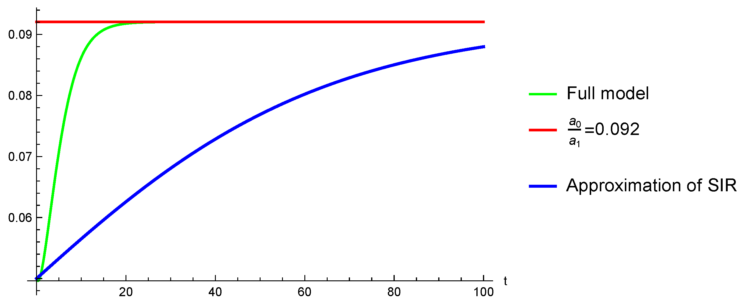
Example 3. 

For the SIR process $\left(S\right(t), I(t), R(t), t\ge 0)$ with linear birth rates $b_s, b_r$ for the susceptible and the recovered, the system for the fractions $\mathsf{s}\left(t\right)=\frac{S\left(t\right)}{N},\mathsf{i}\left(t\right)=\frac{I\left(t\right)}{N},\mathsf{r}\left(t\right)=\frac{R\left(t\right)}{N},N=S+I+R$ is:

$$\left\{\begin{array}{cc}{\mathsf{s}}^{\prime }\left(t\right)=b_s-\beta \mathsf{s}\left(t\right)\mathsf{i}\left(t\right)+{\gamma }_r\mathsf{r}\left(t\right)-d_s\mathsf{s}\left(t\right),\hfill & d_s={\gamma }_s+\mu \hfill \\ {\mathsf{i}}^{\prime }\left(t\right)=\beta \mathsf{s}\left(t\right)\mathsf{i}\left(t\right)-d_i\mathsf{i}\left(t\right),\hfill & d_i={\gamma }_i+\mu +\delta \hfill \\ {\mathsf{r}}^{\prime }\left(t\right)=b_r+{\gamma }_i\mathsf{i}\left(t\right)+{\gamma }_s\mathsf{s}\left(t\right)-d_r\mathsf{r}\left(t\right),\hfill & d_r={\gamma }_r+\mu \hfill \end{array}\right..$$

(11)

The DFE is: $(\frac{b_r{\gamma }_r+b_s\left(\mu +{\gamma }_r\right)}{\mu \left(\mu +{\gamma }_r+{\gamma }_s\right)}, 0, \frac{b_r\left(\mu +{\gamma }_s\right)+b_s{\gamma }_s}{\mu \left(\mu +{\gamma }_r+{\gamma }_s\right)})$.

The rational substitution with respect to i obtained via RUR is:

$$\left(s\to \frac{{\gamma }_r\left(b_r+b_s+i{\gamma }_i\right)+\mu b_s}{\beta i\left(\mu +{\gamma }_r\right)+\mu \left(\mu +{\gamma }_r+{\gamma }_s\right)},r\to \frac{b_r\left(\beta i+\mu +{\gamma }_s\right)+b_s{\gamma }_s+i{\gamma }_i\left(\beta i+\mu +{\gamma }_s\right)}{\beta i\left(\mu +{\gamma }_r\right)+\mu \left(\mu +{\gamma }_r+{\gamma }_s\right)}\right).$$

Note that this reduces to the DFE when $i=0$.

The reduced approximate model obtained via RUR is:

$$\begin{array}{ccc}& & i^{\prime }=i\left[a_0-a_{1}i\right],a_1=\beta \left(\mu {\gamma }_i+(\delta +\mu )\left(\mu +{\gamma }_r\right)\right),\hfill \end{array}$$

(12)

$$\begin{array}{ccc}& & a_0=\beta \left(b_r{\gamma }_r+b_s\left(\mu +{\gamma }_r\right)\right)-\mu \left(\mu +{\gamma }_r+{\gamma }_s\right)\left(\delta +{\gamma }_i+\mu \right)\hfill \\ & & =\mu \left(\mu +{\gamma }_r+{\gamma }_s\right)\left(\delta +{\gamma }_i+\mu \right)\left({\mathsf{s}}_{dfe}\mathcal{R}-1\right)=\mu \left(\mu +{\gamma }_r+{\gamma }_s\right)\left(\delta +{\gamma }_i+\mu \right)\left(R_0-1\right).\hfill \end{array}$$

(13)

This has an explicit (rather formidable) analytic solution, provided in the Mathematica file.

One may notice that for the chosen numerical illustration, the plots of i and its approximation converge towards the same value but differ sharply for the chosen numeric values as far as shape is concerned; see Figure 1.

We mention finally the possibility to develop yet another possible algorithm for computing a “bifurcation $R_0$”, suggested by the example above, which is based on the known fact that this parameter is expected to produce bifurcations at $R_0=1$.

The steps are:

1.

Factor out the variable in the scalar polynomial of the reduced model (always possible if this is a disease variable).

2.

Write the free coefficient of the divided polynomial as $F\left(R_0\right)=G\left(R_0\right)(R_0-1)$, where $F\left(R\right)$ is rational (always possible due to the known bifurcation at $R_0=1$).

3.

Identify a factor which is linear in susceptible variables like ${\mathsf{s}}_{dfe}$, etc., and write it as a difference of positive and negative terms. Upon normalizing one of them to one, the other will be $R_0$, or $1/R_0$.

3. ${\mathit{R}}_{\mathbf{0}}$ and Extinction Probabilities for the SEIR Epidemic Model

The SEIR process $\left(S\right(t),E(t),I(t),R(t),t\ge 0)$ adds to the SIR model the class E(exposed). The model for the fractions $\mathsf{s}\left(t\right)=\frac{S\left(t\right)}{N},\mathsf{e}\left(t\right)=\frac{E\left(t\right)}{N},\mathsf{i}\left(t\right)=\frac{I\left(t\right)}{N},\mathsf{r}\left(t\right)=\frac{R\left(t\right)}{N}, N=S+E+I+R$ is:

$$\left\{\begin{array}{cc}{\mathsf{s}}^{\prime }\left(t\right)=b_s-\beta \mathsf{s}\left(t\right)\mathsf{i}\left(t\right)+{\gamma }_r\mathsf{r}\left(t\right)-d_s\mathsf{s}\left(t\right),\hfill & d_s={\gamma }_s+\mu \hfill \\ {\mathsf{e}}^{\prime }\left(t\right)=\beta \mathsf{s}\left(t\right)\mathsf{i}\left(t\right)-{\gamma }_e\mathsf{e}\left(t\right)-d_e\mathsf{e}\left(t\right),\hfill & d_e={\gamma }_e+\mu \hfill \\ {\mathsf{i}}^{\prime }\left(t\right)={\gamma }_e\mathsf{e}\left(t\right)-d_i\mathsf{i}\left(t\right),\hfill & d_i={\gamma }_i+\mu +\delta \hfill \\ {\mathsf{r}}^{\prime }\left(t\right)=b_r+{\gamma }_i\mathsf{i}\left(t\right)+{\gamma }_s\mathsf{s}\left(t\right)-d_r\mathsf{r}\left(t\right),\hfill & d_r={\gamma }_r+\mu \hfill \end{array}\right..$$

This is both a textbook model and one for which answers to many open questions (concerning, for example, the emergence of chaos under stochastic and periodic perturbations) are still awaited—see for example [38,39,40].

The DFE of (14) is $(\frac{b_r{\gamma }_r+b_s\left(\mu +{\gamma }_r\right)}{\mu \left(\mu +{\gamma }_r+{\gamma }_s\right)},0,0,\frac{b_r\left(\mu +{\gamma }_s\right)+b_s{\gamma }_s}{\mu \left(\mu +{\gamma }_r+{\gamma }_s\right)})$. The decomposition matrices and basic reproduction number are:

$$F=\left(\begin{array}{cc}0& \beta s\\ 0& 0\end{array}\right), V=\left(\begin{array}{cc}{\gamma }_e+\mu & 0\\ -{\gamma }_e& \delta +{\gamma }_i+\mu \end{array}\right), R_0=\frac{\beta s{\gamma }_e}{\left({\gamma }_e+\mu \right)\left(\delta +{\gamma }_i+\mu \right)}.$$

The associated disease stochastic process $X=(e,i)\in {\mathbb{N}}^2$ has a generating operator

$$\mathcal{G}=\underset{¯}{s}i(f(x+e_1)-f\left(x\right))+{\gamma }_{e}e(f(x+tr)-f\left(x\right))+d_{e}e(f(x+e_3)-f\left(x\right))+d_{i}i(f(x+e_2)-f\left(x\right)),$$

where $x=(e,i), e_1=(1,0)=-e_3, tr=(-1,1), e_2=(0,-1)$.

The extinction probabilities obtained by solving (8) are

$$\left\{\begin{array}{cc}{q}_i=1,q_e=1\hfill & \mathrm{when}{R}_0<1\hfill \\ q_i=\frac{1}{R_0},q_e=\frac{\mu }{d_e}+\frac{{\gamma }_e}{d_e}\frac{1}{R_0}\hfill & \mathrm{when}{R}_0\ge 1\hfill \end{array}\right..$$

This checks with the particular case in [13], where ${\mathsf{s}}_{dfe}=1$.

Remark 13. 

It is not clear intuitively why separating the transition rates into those of F (which increase the norm of x) and those of V (which do not increase the norm of x) should matter for determining the extinction probabilities, as happens in (8). This seems to be an interesting question.

4. Rank One Host-Only Models with Pathogen and ${\mathit{R}}_{\mathbf{0}}$ Readable from the Flow-Chart

The SEIARW Model with “Catalyzing Pathogen” of [18] Has Rank One Next-Generation Matrix and $R_0=R_J$

Ref. [18] attempted to offer a “definition-based method” for “computing $R_0$ of dynamic models of single host species, which is mutually coherent with the next-generation method (NGM)” (and somewhat unclear for “computing $R_0$ for a population with multi-group models”). Unfortunately, these authors do not seem aware of the fact that all the single host species they examined have a next-generation matrix of rank one, and that in this case, there exists a simple general formula [20,41,42], which is also related to the definition-based method of [43].

We review now the SEIAR model (susceptibles, exposed, infected, asymptomatic, and recovered), to which [18] add also a pathogen compartment W, resulting in the SEIARW model. See also Figure 2.

$$\left\{\begin{array}{c}\left\{\begin{array}{cc}{e}^{\prime }=s\left(a{\beta }_a+i{\beta }_i+w{\beta }_w\right)-e{d}_e,\hfill & d_e=e_i+e_a+\mu \hfill \\ i^{\prime }=e{e}_i-i{d}_i,\hfill & d_i={\gamma }_i+\mu +\delta ,\hfill \\ a^{\prime }=e{e}_a-a{d}_a,\hfill & d_a={\gamma }_a+\mu ,\hfill \\ w^{\prime }=a{ϵ}_a+i{ϵ}_i-w{d}_w\hfill \\ r^{\prime }=a{\gamma }_a+{\gamma }_{i}i-\mu r\hfill \end{array}\right.\hfill \\ s^{\prime }=\Lambda -s\left(a{\beta }_a+i{\beta }_i+w{\beta }_w+\mu \right).\hfill \end{array}\right.$$

(14)

In matrix form, the disease equations are:

$$\begin{array}{c}\hfill \left(\begin{array}{c}{e}^{\prime }\\ i^{\prime }\\ a^{\prime }\\ w^{\prime }\\ r^{\prime }\end{array}\right)=\left(\begin{array}{ccccc}-d_e& s{\beta }_i& s{\beta }_a& s{\beta }_w& 0\\ e_i& -d_i& 0& 0& 0\\ e_a& 0& -d_a& 0& 0\\ 0& {ϵ}_i& {ϵ}_a& -d_w& 0\\ 0& {\gamma }_i& {\gamma }_a& 0& -\mu \end{array}\right)\left(\begin{array}{c}e\\ i\\ a\\ w\\ r\end{array}\right).\end{array}$$

In the absence of a pathogen, SEIAR is a rank one “generalized stage-structured infectious disease model” as revealed by its $F=\left(\begin{array}{ccc}0& s{\beta }_i& s{\beta }_a\\ 0& 0& 0\\ 0& 0& 0\end{array}\right)$ and by its $V=\left(\begin{array}{ccc}{d}_e& 0& 0\\ -e_i& d_i& 0\\ -e_a& 0& d_a\end{array}\right)$ matrix, which is triangular (compare to ([14] (Section 3))).

The $R_0$ has a very intuitive and easily explainable form:

$$R_0=\frac{{\mathsf{s}}_{dfe}}{d_e}{}_{\stackrel{++}{=}}{\beta }_i\frac{e_i}{d_i}+{\beta }_a\frac{d_a}{e_a}$$

(15)

(compare to ([14] (Section 3)) to see the general pattern for more stages).

Remark 14. 

Note that this result may be obtained with $\mathcal{I}=\{e,i,a,r\}$ and also with $\mathcal{I}=\{e,i,a\},$ which raises the question of defining the concept of a minimal or “sufficient disease” set in such a way that it allows for deriving both $R_0$ and the extinction probabilities.

After the addition of the catalyzing pathogen, the SEIARW is still a rank one “generalized stage-structured infectious disease model”, but the $R_0$ is less intuitive

$$R_0=\frac{{\mathsf{s}}_{dfe}}{d_e}[{\beta }_i\frac{e_i}{d_i}+{\beta }_a\frac{d_a}{e_a}+\frac{{\beta }_w}{d_w}\left({ϵ}_i\frac{e_i}{d_i}+{ϵ}_a\frac{e_a}{d_a}\right)];$$

(16)

still, it may be read out of the flow chart “almost by inspection” (see also [18] for an algorithm computing this).

Despite the fact that the characteristic polynomial is not of the Descartes type, all our three $R_0$ recipes yield the above result. We provide now details for the NGM method. After removing the compartment r (since it does not appear in the other equations), the calls “inf=Range[4];DFE[SEIARW,inf]; NGM[SEIARW,inf]” of our scripts yield that the DFE is

$$\left\{s\to \frac{\Lambda }{\mu },e\to 0,i\to 0,a\to 0,w\to 0\right\}$$

and

$$F=s\left(\begin{array}{cccc}0& {\beta }_i& {\beta }_a& {\beta }_w\\ 0& 0& 0& 0\\ 0& 0& 0& 0\\ 0& 0& 0& 0\end{array}\right)=s\left(\begin{array}{c}1\\ 0\\ 0\\ 0\end{array}\right)\left(\begin{array}{cccc}0& {\beta }_i& {\beta }_a& {\beta }_w\end{array}\right),V=\left(\begin{array}{cccc}{d}_e& 0& 0& 0\\ -e_i& d_i& 0& 0\\ -e_a& 0& d_a& 0\\ 0& -{ϵ}_i& -{ϵ}_a& d_w\end{array}\right).$$

(17)

Here the dominant eigenvalue of $K=F{V}^{-1}$, that of the transpose

$$K^t=s\left(\begin{array}{cccc}\frac{{\beta }_i{d}_w{e}_i{d}_a+{\beta }_a{e}_a{d}_w{d}_i+{\beta }_w\left(e_i{ϵ}_i{d}_a+e_a{ϵ}_a{d}_i\right)}{d_e{d}_i{d}_a{d}_w}& \frac{{\beta }_i{d}_w+{ϵ}_i{\beta }_w}{d_w{d}_i}& \frac{{\beta }_a{d}_w+{ϵ}_a{\beta }_w}{d_w{d}_a}& \frac{{\beta }_w}{d_w}\\ 0& 0& 0& 0\\ 0& 0& 0& 0\\ 0& 0& 0& 0\end{array}\right),$$

the rank 1 formula of [20,41,42]

$$(1,0,0,0).{\left(V^t\right)}^{-1}.{(0,{\beta }_i,{\beta }_a,{\beta }_w)}^t,$$

as well as the Jacobian factorization confirm all the results (16) of [18].

5. Target-Infection-Virus Models

5.1. Two Admissible $(F,V)$ Decompositions and $R_0$’s for the Three Dimensional Model of [44]

The three dimensional model of ([44] eq(1)) is:

$$\left\{\begin{array}{c}{x}^{\prime }=\Lambda \left(x\right)-\beta xv-{\beta }_{xy}xy,\Lambda \left(x\right)={\mu }_x(x_{dfe}-x)\hfill \\ \left(\begin{array}{c}{y}^{\prime }\\ v^{\prime }\end{array}\right)=\left(\begin{array}{c}\beta xv+{\beta }_{xy}xy\\ 0\end{array}\right)-\left(\begin{array}{c}{\mu }_{y}y\\ {\mu }_{v}v+{\beta }_{xv}xv+{\beta }_{yv}yv-b{\mu }_{y}y\end{array}\right),\hfill \end{array}\right.$$

(18)

where we represented already the infectious equations as a difference of “new (positive) infection” terms and “transfers”. The DFE is $x=x_{dfe}, y=0, v=0$.

This reduces to the case with zero delays in ([45] eq(5.1)), when the rate of viruses moving into a healthy cell ${\beta }_{xv}$ and the rate of viruses moving into an infected cell ${\beta }_{yv}$ are both 0, and to the case in [46], when ${\beta }_{yv}=0={\beta }_{xy}$ (the latter is the cell-to-cell infection rate) and ${\beta }_{xv}=\beta$.

The gradient of the infectious equations is

$$M=\left(\begin{array}{cc}x{\beta }_{xy}-{\mu }_y& \beta x\\ b{\mu }_y-v{\beta }_{yv}& -{\mu }_v-x{\beta }_{xv}-y{\beta }_{yv}\end{array}\right).$$

(19)

Calling our NGM script with “inf = {2,3}” yields [44]’s result: namely,

$$F=x_{dfe}\left(\begin{array}{cc}{\beta }_{xy}& \beta \\ 0& 0\end{array}\right), -V=\left(\begin{array}{cc}-{\mu }_y& 0\\ b{\mu }_y& -{\mu }_v-x_{dfe}{\beta }_{xv}\end{array}\right),$$

the next-generation matrix (NGM) of the infectious coordinates at the DFE

$$K=\left(\begin{array}{cc}\frac{\beta bx}{{\mu }_v+x{\beta }_{xv}}+\frac{x{\beta }_{xy}}{{\mu }_y}& \frac{\beta x}{{\mu }_v+x{\beta }_{xv}}\\ 0& 0\end{array}\right),$$

and that the DFE is Lyapunov–Malkin stable when $R_0$ defined in

$$R_0=\frac{x_{dfe}}{x_c}+\beta b\frac{x_{dfe}}{{\mu }_v+x_{dfe}{\beta }_{xv}},x_c:=\frac{{\mu }_y}{{\beta }_{xy}},$$

(20)

is smaller than 1 and unstable when $R_0>1$.

The Jacobian factorization provides the same formula, despite the fact that the characteristic polynomial is of the Descartes type only conditionally, when ${\beta }_{xv}\ge {\beta }_{xy}$.

Remark 15. 

Interestingly, another admissible decomposition $\mathcal{F}=\left(\begin{array}{c}\beta xv+{\beta }_{xy}xy\\ beta{\mu }_{y}y\end{array}\right)$, appears in an earlier version of [44] at https://people.clas.ufl.edu/pilyugin/files/cosner60-dcdsB.pdf (accessed on 1 November 2023):

$$F=\left(\begin{array}{cc}x{\beta }_{xy}& \beta x\\ b{\mu }_y& 0\end{array}\right),V=\left(\begin{array}{cc}{\mu }_y& 0\\ 0& {\mu }_v+{\beta }_{xv}{x}_{dfe}\end{array}\right),K=\left(\begin{array}{cc}\frac{x_{dfe}}{x_c}& \frac{\beta x_{dfe}}{{\mu }_v+{\beta }_{xv}{x}_{dfe}}\\ b& 0\end{array}\right)$$

(21)

This second decomposition yields a different $R_0$:

$$R_0=\frac{x_{dfe}}{2x_c}\left(1+\sqrt{1+\frac{4\beta b{x}_c^2}{x_{dfe}(x_{dfe}{\beta }_{xv}+{\mu }_v)}}\right).$$

(22)

Furthermore, this early version also shows that the two decompositions have the same stability domain for the DFE, which may be reexpressed as

$$R_0=K_{1,1}+K_{1,2}{K}_{2,1}=\frac{x_{dfe}}{x_c}+b\beta \frac{x_{dfe}}{{\mu }_v+{\beta }_{xv}{x}_{dfe}}<1.$$

(23)

We note that this equivalence also follows by applying the first criterion in [47] (when the characteristic polynomial, given here by ${\lambda }^n-a_1{\lambda }^{n-1}-a_2{\lambda }^{n-1}-...$ has all coefficients as non-negative, then ${\sum }_i{a}_i$ may be used as the threshold parameter instead of $R_0$), with $n=3, a_1=K_{1,1}, a_2=K_{1,2}{K}_{2,1}, a_3=0$.

Remark 16. 

Note the second decomposition has one more non-zero term in F, which does not appear in ours, since we view it as a transfer and not as an interaction. We see here an excellent example of non-uniqueness, where one must choose between an answer with F of a lower rank and a simpler $R_0$ formula, but which is valid only under certain conditions (that the non-diagonal term $b{\mu }_y$ in V is small enough), and an answer with a simpler V, which requires less assumptions on the parameters but yields a more complicated $R_0$.

Remark 17. 

The domain of stability, in terms of the parameters. As an aside, it is easy to show that (23) is equivalent to

$$x_{dfe}<x_c, b<b_0:=\frac{{\mu }_v+{\beta }_{xv}{x}_{dfe}}{\beta x_{dfe}}\left(1-\frac{x_{dfe}}{x_c}\right),$$

(24)

where $b_0$ is the solution of equation $R_0\left(b\right)=1$. Thus, the stability of the DFE is equivalent to both $x_{dfe}$ and the “burst parameter” b being small enough.

We offer now a third gradient decomposition, which turns out to be inadmissible sometimes, but it again yields our recipe’s $R_0$. Taking $F=\left(\begin{array}{cc}{x}_{dfe}{\beta }_{xy}& 0\\ b{\mu }_y& 0\end{array}\right)$ yields

$$V=F-M=\left(\begin{array}{cc}{\mu }_y& -\beta x_{dfe}\\ 0& {\mu }_v+x_{dfe}{\beta }_{xv}\end{array}\right),V^{-1}=\left(\begin{array}{cc}\frac{1}{{\mu }_y}& \frac{\beta x_{dfe}}{{\mu }_y({\mu }_v+x_{dfe}{\beta }_{\mathrm{xv}})}\\ 0& \frac{1}{{\mu }_v+x_{dfe}{\beta }_{\mathrm{xv}}}\end{array}\right).$$

Note that V is a sub-generating matrix only if $x_{dfe}\le \frac{{\mu }_y}{\beta }$.

However $K=\left(\begin{array}{cc}\frac{x_{dfe}{\beta }_{xy}}{{\mu }_y}& \frac{\beta x_{dfe}^2{\beta }_{xy}}{{\mu }_v{\mu }_y+x_{dfe}{\beta }_{xv}{\mu }_y}\\ b& \frac{\beta b{x}_{dfe}}{{\mu }_v+x_{dfe}{\beta }_{xv}}\end{array}\right)$ yields the correct

$$R_0=max\left(0,\frac{\beta b{x}_{dfe}}{{\mu }_v+x_{dfe}{\beta }_{xv}}+\frac{x_{dfe}{\beta }_{xy}}{{\mu }_y}\right).$$

In the current example, the RUR algorithm works as well. The difference of the two positive terms is

$$\beta b{x}_{dfe}{\mu }_y+x_{dfe}{\beta }_{xy}({\mu }_v+x_{dfe}{\beta }_{xv})-{\mu }_y({\mu }_v+x_{dfe}{\beta }_{xv})={\mu }_y({\mu }_v+x_{dfe}{\beta }_{xv})(R_0-1),$$

for both choices y and v as scalar variables, and the appropriate cosmetics recover the recipe NGM $R_0$.

This example illustrates the fact that sometimes several admissible and even conditionally non-admissible decompositions, as well as other approaches, may lead to the same $R_0$.

5.2. Two Distinct Approximate Extinction Probabilities, One for Each Admissible $(F,V)$ Decomposition for the Model of [44]

The extinction probabilities of the stochastic model are of course unique. We may use the result of Bacaer’s formula as approximations. In this interesting example, we find out that both $(F,V)$ decompositions yield reasonable results. This suggests that we have not one, but two deterministic epidemiologic approximations for a single stochastic model. This strengthens our point of view that a deterministic epidemiologic model must include a specification of the $(F,V)$ decomposition.

The respective results we obtained are:

1.

For the first decomposition, the extinction probabilities obtained by solving (8) are

$$\begin{array}{c}\hfill \left\{\begin{array}{c}{q}_y=1,q_z=1,\mathrm{when}{R}_0\le 1,\hfill \\ q_y=\frac{\pm \sqrt{x^2\left(\left({\beta }_{\mathrm{xy}}\left({\mu }_{\mathrm{v}}+x\left(\beta +{\beta }_{\mathrm{xv}}\right)\right)+\beta {\mu }_{\mathrm{y}}\right){}^2-4\beta {\beta }_{\mathrm{xy}}{\mu }_{\mathrm{y}}\left(x\left(\beta -b\beta +{\beta }_{\mathrm{xv}}\right)+{\mu }_{\mathrm{v}}\right)\right)}+x\left({\mu }_{\mathrm{v}}{\beta }_{\mathrm{xy}}+\beta {\mu }_{\mathrm{y}}\right)+x^2\left(\beta +{\beta }_{\mathrm{xv}}\right){\beta }_{\mathrm{xy}}}{2\beta x^2{\beta }_{\mathrm{xy}}},\mathrm{when}{R}_0>1\hfill \\ q_z=\frac{\left({\mu }_{\mathrm{v}}+x{\beta }_{\mathrm{xv}}\right)\left(\pm \sqrt{x^2\left(\left({\beta }_{\mathrm{xy}}\left({\mu }_{\mathrm{v}}+x\left(\beta +{\beta }_{\mathrm{xv}}\right)\right)+\beta {\mu }_{\mathrm{y}}\right){}^2-4\beta {\beta }_{\mathrm{xy}}{\mu }_{\mathrm{y}}\left(x\left(\beta -b\beta +{\beta }_{\mathrm{xv}}\right)+{\mu }_{\mathrm{v}}\right)\right)}-x{\mu }_{\mathrm{v}}{\beta }_{\mathrm{xy}}+x^2\left(\beta +{\beta }_{\mathrm{xv}}\right)\left(-{\beta }_{\mathrm{xy}}\right)+\beta x{\mu }_{\mathrm{y}}\right)}{2{\beta }^{2}b{x}^2{\mu }_{\mathrm{y}}}.\hfill \end{array}\right.\end{array}$$

2.

For the second decomposition, the extinction probabilities obtained by solving (8) are:

$$\begin{array}{c}\hfill \left\{\begin{array}{c}{q}_y=1,q_z=1,\mathrm{when}{R}_0\le 1,\hfill \\ q_y=\frac{\pm \sqrt{x^2\left(\left(\beta (b+1){\mu }_{\mathrm{y}}+{\beta }_{\mathrm{xy}}\left({\mu }_{\mathrm{v}}+x\left(\beta +{\beta }_{\mathrm{xv}}\right)\right)\right){}^2-4\beta {\beta }_{\mathrm{xy}}{\mu }_{\mathrm{y}}\left({\mu }_{\mathrm{v}}+x\left(\beta +{\beta }_{\mathrm{xv}}\right)\right)\right)}+\beta (b+1)x{\mu }_{\mathrm{y}}+x{\mu }_{\mathrm{v}}{\beta }_{\mathrm{xy}}+x^2\left(\beta +{\beta }_{\mathrm{xv}}\right){\beta }_{\mathrm{xy}}}{2\beta x^2{\beta }_{\mathrm{xy}}},\mathrm{when}{R}_0>1,\hfill \\ q_z=\frac{\left({\mu }_{\mathrm{v}}+x{\beta }_{\mathrm{xv}}\right)\left(\pm \sqrt{x^2\left(\left(\beta (b+1){\mu }_{\mathrm{y}}+{\beta }_{\mathrm{xy}}\left({\mu }_{\mathrm{v}}+x\left(\beta +{\beta }_{\mathrm{xv}}\right)\right)\right){}^2-4\beta {\beta }_{\mathrm{xy}}{\mu }_{\mathrm{y}}\left({\mu }_{\mathrm{v}}+x\left(\beta +{\beta }_{\mathrm{xv}}\right)\right)\right)}+\beta (b+1)x{\mu }_{\mathrm{y}}-x{\mu }_{\mathrm{v}}{\beta }_{\mathrm{xy}}+x^2\left(\beta +{\beta }_{\mathrm{xv}}\right)\left(-{\beta }_{\mathrm{xy}}\right)\right)}{2\beta bx{\mu }_{\mathrm{y}}\left({\mu }_{\mathrm{v}}+x\left(\beta +{\beta }_{\mathrm{xv}}\right)\right)}.\hfill \end{array}\right.\end{array}$$

In a numeric instance, we found the two results reasonably close to each other.

6. Multi-Strain Host-Only Models

Multi-strain diseases are diseases that consist of several strains, or serotypes. One interesting thing about multi-strain models is that, besides the DFE, we have new boundary points which are relevant epidemiologically, in which one subset of strains A is present (“resident”). We have then a natural coexistence of several “$\mathcal{R}$ thresholds”:

1.

$R_A$ is the bifurcation threshold at which the DFE stops being stable, when the only compartments present are those of A.

2.

${\mathcal{R}}_A$ is the bifurcation threshold at which the boundary point $E_A$ starts existing (in the presence of the $A^c$ compartments).

3.

$R_{A^c,A}$ is the bifurcation threshold at which the boundary point $E_A$ stops being stable, i.e., when the $A^c$ compartments invade the A compartments.

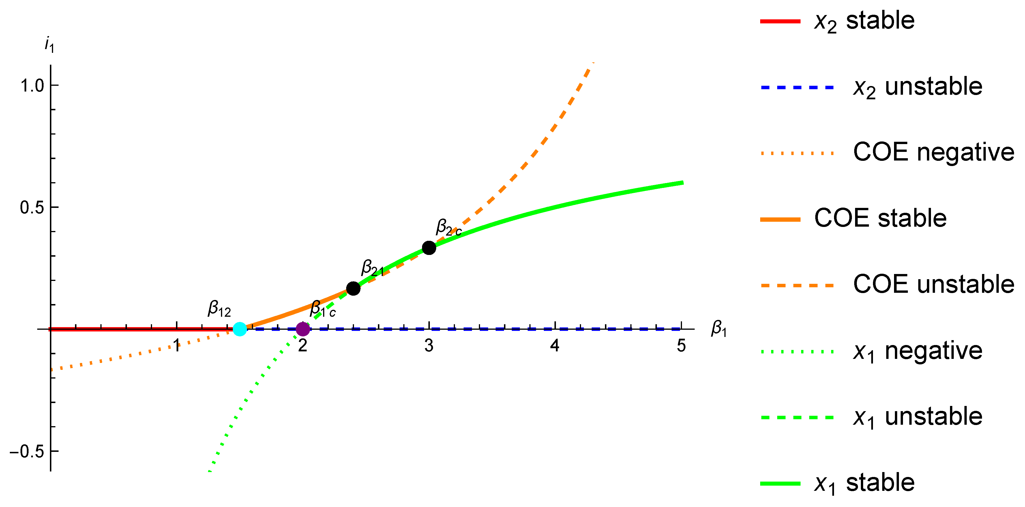
Note that for two strains already, we have at least two new thresholds, $R_{21}, R_{12},$ which, together with $R_0$ and the thresholds $R_1$, $R_2$ of the individual strains, divide the line into six regions with different stability properties. Studying the relations between the various thresholds in the parameter space is quite a challenging topic. However, their calculation is a priori of the same level of difficulty as for the DFE.

6.1. The Two-Strain SIS Tuberculosis Model of ([22] (Section 4.4))

The model presented here is a limiting case of that presented in the next section, obtained when the transition rates ${\gamma }_1,{\gamma }_2$ converge to ∞. It also generalizes the two-strain SIS tuberculosis model of ([22] (Section 4.4)) by allowing for cross infections in both directions

$$\begin{array}{c}\hfill \left\{\begin{array}{c}{i}_1^{\prime }=i_1\left(i_2\left({\nu }_2-{\nu }_1\right)+{\beta }_{1}s-{\sigma }_1-b\right)=i_1\left(i_2\left({\nu }_2-{\nu }_1\right)+{\beta }_{1}s-d_1\right),\hfill \\ i_2^{\prime }=i_2\left(i_1\left({\nu }_1-{\nu }_2\right)+{\beta }_{2}s-{\sigma }_2-b\right)=i_2\left(i_1\left({\nu }_1-{\nu }_2\right)+{\beta }_{2}s-d_2\right),\hfill \\ s^{\prime }=b-s\left({\beta }_1{i}_1+{\beta }_2{i}_2+b\right)+i_1{\sigma }_1+i_2{\sigma }_2,\hfill \end{array}\right.\end{array}$$

where we put $d_1={\sigma }_1-b, d_2={\sigma }_2-b$ in the first two equations to simplify their notation (the last equation may be removed, since $s=1-i_1-i_2$).

Noting that the first two equations’ factor yields the following three boundary steady states, where $\mathbf{x}=(i_1,i_2,s)$:

$$\begin{array}{ccc}\hfill {\mathbf{x}}_0& =& \left(0,0,1\right),\hfill \end{array}$$

(25)

$$\begin{array}{ccc}\hfill {\mathbf{x}}_1& =& {\displaystyle \left(1-{\mathcal{R}}_1^{-1},0,{\mathcal{R}}_1^{-1}\right),}\hfill \end{array}$$

(26)

$$\begin{array}{ccc}\hfill {\mathbf{x}}_2& =& {\displaystyle \left(0,1-{\mathcal{R}}_2^{-1},{\mathcal{R}}_2^{-1}\right),}\hfill \end{array}$$

where we put

$${\displaystyle {\mathcal{R}}_1=\frac{{\beta }_1}{b+{\sigma }_1},{\mathcal{R}}_2=\frac{{\beta }_2}{b+{\sigma }_2}.}$$

The disease-free steady state ${\mathbf{x}}_0$ exists for all parameter values, while the original strain-only steady state ${\mathbf{x}}_1$ is physically relevant if and only if ${\mathcal{R}}_1>1$, and the emerging strain-only steady state ${\mathbf{x}}_2$ is physically relevant if and only if ${\mathcal{R}}_2>1$.

There may also be a fourth non-negative coexistence equilibrium (COE), given by

$$\left\{\begin{array}{c}{i}_1=\frac{{\beta }_1{d}_2-{\beta }_2{d}_1-\left({\nu }_1-{\nu }_2\right)\left({\beta }_2-d_2\right)}{\left({\nu }_1-{\nu }_2\right)\left({\beta }_1-{\beta }_2+{\nu }_1-{\nu }_2\right)}\hfill \\ i_2=\frac{d_1\left({\beta }_2-{\nu }_1+{\nu }_2\right)-{\beta }_1\left(d_2-{\nu }_1+{\nu }_2\right)}{\left({\nu }_1-{\nu }_2\right)\left({\beta }_1-{\beta }_2+{\nu }_1-{\nu }_2\right)}\hfill \\ s=1-i_1-i_2\hfill \end{array}\right..$$

(27)

Note that this depends only on ${\nu }_1-{\nu }_2,$ which shows that the case ${\nu }_1=0$ considered in ([22] (Section 4.4)) is not that restrictive (However, the appearance of ${\nu }_1-{\nu }_2$ in the denominator suggests limiting the diffusion phenomena, which may be worth studying in their own right.) In this case, the COE point simplifies to:

$$\left\{\begin{array}{c}{i}_1=\frac{d_2\left(d_1\left({\mathcal{R}}_1-{\mathcal{R}}_2\right)+\nu \left({\mathcal{R}}_2-1\right)\right)}{\nu \left(-d_1{\mathcal{R}}_1+d_2{\mathcal{R}}_2+\nu \right)}\hfill \\ i_2=\frac{d_1\left(d_2\left({\mathcal{R}}_2-{\mathcal{R}}_1\right)+\nu (1-{\mathcal{R}}_1)\right)}{\nu \left(-d_1{\mathcal{R}}_1+d_2{\mathcal{R}}_2+\nu \right)}\hfill \\ s=1-i_1-i_2\hfill \end{array}\right.,$$

(28)

which is positive if ${\mathcal{R}}_2>1$ and the following conditions hold

$$\left\{\begin{array}{c}{\mathcal{R}}_1>\frac{\nu +{\mathcal{R}}_2{d}_2}{\nu +d_2},0<\nu <\frac{d_1({\mathcal{R}}_2-{\mathcal{R}}_1)}{{\mathcal{R}}_2-1},\mathrm{or},\hfill \\ {\mathcal{R}}_1<\frac{\nu +{\mathcal{R}}_2{d}_2}{\nu +d_2},\left(0<d_1<\nu (1-\frac{1}{{\mathcal{R}}_2})\mathrm{or}{d}_1>\nu (1-\frac{1}{{\mathcal{R}}_2}),\nu <\frac{d_1({\mathcal{R}}_2-{\mathcal{R}}_1)}{1-{\mathcal{R}}_2}\right).\hfill \end{array}\right.$$

(29)

We give now some details of the NGM implementation for the three boundary points. Recall that the idea is to project the ODE at each boundary point on the 0 coordinates (or some subset), while fixing the other coordinates. We must therefore compute new $(F,V)$ pairs at each boundary point, since the respective zero coordinates are different.

1.

At the DFE, the zero coordinates are $\left\{i_1,i_2\right\}$, and so $\mathcal{I}=\{1,2\}$.

Our script yields the expected result

$$R_0=Max\left[\frac{{\beta }_2{s}_{dfe}}{{\sigma }_2+b},\frac{{\beta }_1{s}_{dfe}}{{\sigma }_1+b}\right]=Max\left[R_1,R_2\right],R_i={\mathsf{s}}_{dfe}{\mathcal{R}}_i={\mathcal{R}}_i,i=1,2.$$

2.

At ${\mathbf{x}}_2$, $\mathcal{I}=\left\{1\right\}$, and

$$R_{12}=\frac{{\mathcal{R}}_1}{{\mathcal{R}}_2}+\frac{\left({\nu }_2-{\nu }_1\right)\left(1-{\mathcal{R}}_2^{-1}\right)}{b+{\sigma }_1}.$$

When ${\nu }_1=0,{\nu }_2=\nu ,$ we recover the result ([22] (18)) $R_{12}=\frac{{\mathcal{R}}_1}{{\mathcal{R}}_2}+\frac{\nu }{b+{\sigma }_1}\left(1-{\mathcal{R}}_2^{-1}\right).$

This implies that the stability holds if ${\mathcal{R}}_2>1$ and ${\mathcal{R}}_1$ are not too big, more precisely:

$$R_{12}<1\iff {\mathcal{R}}_1<{\mathcal{R}}_2+\frac{\nu \left(1-{\mathcal{R}}_2\right)}{b+{\sigma }_1}.$$

(30)

For a sanity check, we will derive the stability condition of the point ${\mathbf{x}}_2$ also by the direct Jacobian approach. The Jacobian at ${\mathbf{x}}_2$ is

$$\left(\begin{array}{ccc}\frac{-{\beta }_2\left(b+{\nu }_1-{\nu }_2+{\sigma }_1\right)+{\beta }_1\left(b+{\sigma }_2\right)+\left({\nu }_1-{\nu }_2\right)\left(b+{\sigma }_2\right)}{{\beta }_2}& 0& 0\\ -\frac{\left({\nu }_1-{\nu }_2\right)\left(b-{\beta }_2+{\sigma }_2\right)}{{\beta }_2}& 0& -b+{\beta }_2-{\sigma }_2\\ {\sigma }_1-\frac{{\beta }_1\left(b+{\sigma }_2\right)}{{\beta }_2}& -b& {\sigma }_2-{\beta }_2\end{array}\right).$$

In the case of [22], the eigenvalues are

$$\left\{-b,-\left(\left({\mathcal{R}}_2-1\right)\left(b+{\sigma }_2\right)\right),\frac{(b+{\sigma }_1)\left({\mathcal{R}}_1-{\mathcal{R}}_2\right)+\nu \left({\mathcal{R}}_2-1\right)}{{\mathcal{R}}_1}\right\}.$$

The second eigenvalue is negative if ${\mathcal{R}}_2>1$, and the third eigenvalue is negative when

$$\left({\mathcal{R}}_1-{\mathcal{R}}_2\right)+\frac{\nu }{b+{\sigma }_1}\left({\mathcal{R}}_2-1\right)<0\iff R_{12}<1\mathrm{see}\left(30\right).$$

3.

An analog result holds via symmetry at ${\mathbf{x}}_1$, where $\mathcal{I}=\left\{2\right\}$, and

$${\mathcal{R}}_{21}=\frac{\left({\nu }_1-{\nu }_2\right)\left({\mathcal{R}}_1-1\right)}{d_2{\mathcal{R}}_1}+\frac{{\mathcal{R}}_2}{{\mathcal{R}}_1}.$$

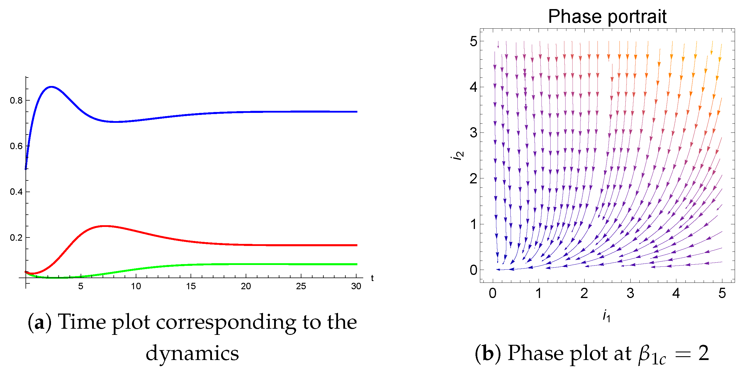
We illustrate now in Figure 3 via an $i_1$ bifurcation diagram that, as natural, when ${\beta }_1$ is small enough, the $x_2$ fixed point is stable enough to be replaced as an attractor, first by the COE, and finally by the $x_1$ fixed point, when ${\beta }_1$ increases. Figure 4 illustrate time and phase plots at the critical point ${\beta }_{1c}=2$.

6.2. The Minimal Disease Set of the Multi-Strain Host-Only Dengue Model with Antibody-Dependent Enhancement (ADE) [48]

The ADE (antibody-dependent enhancement) effect, believed to occur for dengue and Zika, means that infection with a single serotype is asymptomatic, but infection with a second serotype may lead to serious illness accompanied by greater infectivity. It was first studied mathematically by [49,50], who showed that for sufficiently small ADE, the numbers of infectives of each serotype synchronize, with outbreaks occurring in phase, but when the ADE increases past a threshold, the system becomes chaotic, and infectives of each serotype desynchronize (however, certain groupings of the primary and secondary infectives remain synchronized even in the chaotic regime). Subsequently, Ref. [51] examined the effects of single-strain vaccine campaigns on the dynamics of an epidemic multi-strain dengue model. We cite now the eloquent dengue description given by these authors:

“What makes modeling the dengue virus so interesting is that it has developed a sophisticated spreading process. Dengue is known to exhibit as many as four coexisting serotypes (strains) in a region. Once a person is infected and recovered from one serotype, they confer life-long immunity from that serotype. However, the antibodies that the body develops for the first serotype will not counteract a second infection by a different serotype. In fact, due to the nature of the disease, the antibodies developed from the first infection form complexes with the second serotype so that the virus can enter more cells, increasing viral production. The increased transmission rate in subsequent infections is known as antibody-dependent enhancement (ADE). ADE is an alarming evolutionary development in multistrain viruses with respect to vaccines. An optimal vaccination would need to cover all strains of the disease at once, or the vaccinations could increase transmission of the strains not covered. This is particularly dangerous for people who have dengue because the infections are more severe in individuals who already have dengue antibodies”.

A multi-strain model which adds further compartments allowing for temporary cross-immunity has been developed in the works of Aguiar, Stollenwerk, and Kooi [48,52,53,54,55].

In this section, we consider a ten-compartmentasymmetric version of the model of [48], whose variables, denoted by capital letters, represent

1.

S as individuals susceptible to both strains;

2.

$I_i$, for $i,j=1,2$, as individuals infected with strain i and with temporary cross-immunity to strain $j\ne i$;

3.

$R_i$ as individuals who have recovered from strain i, but are not yet susceptible to the other strain j;

4.

$S_i$ as individuals who have recovered from strain i, and have become susceptible to the other strain j;

5.

$Y_j=I_{ij}$ as individuals previously infected with strain i and are now immune to it, but became reinfected with strain $j,i,j=1,2,i\ne j$;

6.

R, omitted in (31) since they do not feed back to the other components, as the recovered individuals immune to all the strains.

After denoting by small letters the corresponding proportions, we arrive at:

$$\left\{\begin{array}{c}{s}^{\prime }=\mu -s\left({\beta }_1{i}_1+{\beta }_2{i}_2+\mu +{\beta }_1{y}_1{\varphi }_1+{\beta }_2{y}_2{\varphi }_2\right),\hfill \\ i_1^{\prime }={\beta }_{1}s\left(i_1+y_1{\varphi }_1\right)-i_1\left({\gamma }_1+\mu \right),\hfill \\ r_1^{\prime }={\gamma }_1{i}_1-r_1\left({\theta }_1+\mu \right),\hfill \\ s_1^{\prime }={\theta }_1{r}_1-s_1\left({\beta }_2{\alpha }_2\left(i_2+y_2{\varphi }_2\right)+\mu \right),\hfill \\ y_2^{\prime }={\beta }_2{\alpha }_2{s}_1\left(i_2+y_2{\varphi }_2\right)-y_2\left({\gamma }_2+\mu \right),\hfill \\ i_2^{\prime }={\beta }_{2}s\left(i_2+y_2{\varphi }_2\right)-i_2\left({\gamma }_2+\mu \right),\hfill \\ r_2^{\prime }={\gamma }_2{i}_2-r_2\left({\theta }_2+\mu \right),\hfill \\ s_2^{\prime }={\theta }_2{r}_2-s_2\left({\beta }_1{\alpha }_1\left(i_1+y_1{\varphi }_1\right)+\mu \right),\hfill \\ y_1^{\prime }={\beta }_1{\alpha }_1{s}_2\left(i_1+y_1{\varphi }_1\right)-y_1\left({\gamma }_1+\mu \right).\hfill \end{array}\right.$$

(31)

In addition to the DFE where $s=1$ and all the other compartments are 0, this system also has two other boundary points. With ${\mathcal{R}}_i=\frac{{\beta }_i}{{\gamma }_i+\mu }$, these are:

1.

one with $i_2=r_2=s_2=y_1=y_2=0$, given by

$$\begin{array}{c}\hfill E_1=\left(\frac{\mu }{{\beta }_1}\left({\mathcal{R}}_1-1\right),\frac{\mu {\gamma }_1}{{\beta }_1\left({\alpha }_1+\mu \right)}({\mathcal{R}}_1-1),\frac{{\alpha }_1{\gamma }_1}{{\beta }_1\left({\alpha }_1+\mu \right)}({\mathcal{R}}_1-1),0,0,0,0,0,\frac{1}{{\mathcal{R}}_1}\right),\end{array}$$

2.

and one with $i_1=r_1=s_1=y_1=y_2=0$, given by

$$\begin{array}{c}\hfill E_2=\left(0,0,0,0,\frac{\mu }{{\beta }_2}\left({\mathcal{R}}_2-1\right),\frac{\mu {\gamma }_2}{{\beta }_2\left({\alpha }_2+\mu \right)}({\mathcal{R}}_2-1),\frac{{\alpha }_2{\gamma }_2}{{\beta }_2\left({\alpha }_2+\mu \right)}({\mathcal{R}}_2-1),0,\frac{1}{{\mathcal{R}}_2}\right).\end{array}$$

(32)

Thus, ${\mathcal{R}}_i,i=1,2$ are the bifurcation values at which these two boundary points appear.

The maximal disease set contains $I_i,R_i,S_i,Y_i,i=1,2$. The DFE may be determined already using the disease set $I_i,Y_i,i=1,2$, which has the advantage of possessing a simple characteristic polynomial with two factors $R_1\left(X\right), R_2\left(X\right)$, which yields:

$$R_J=max[R_1\left(X\right), R_2\left(X\right)], R_1\left(X\right)=\frac{{\beta }_2\left({\alpha }_2{s}_1{\varphi }_2+s\right)}{{\gamma }_2+\mu }, R_2\left(X\right)=\frac{{\beta }_1\left({\alpha }_1{s}_2{\varphi }_1+s\right)}{{\gamma }_1+\mu }.$$

Also, our scripts find that

$$R_{ji}={\mathsf{s}}_{dfe}{\mathcal{R}}_j,j\ne i,i=1,2.$$

(33)

Finally, applying the NGM script to $E_i,i=1,2$ yields the elegant relation

$$R_0={\mathsf{s}}_{dfe}max\left[{\mathcal{R}}_1,{\mathcal{R}}_2\right]=max\left[R_{21},R_{12}\right].$$

(34)

Remark 18. 

Note the notations $R_1\left(X\right), R_2\left(X\right)$, suggesting that we want to view these as polynomials in the variables of the model, rather than as values evaluated at one of the fixed points.

We end this section by drawing the attention to the object which allowed for computing the key polynomials $R_1\left(X\right), R_2\left(X\right)$.

Definition 2. 

(A) A minimal disease set $\mathcal{I}$ is a minimal set which still allows the computation of the DFE, after being set to 0.

(B) The model factors are the factors which may admit positive roots in the characteristic polynomial of the Jacobian with all variables in $\mathcal{I}$ set to 0.

Remark 19. 

Assume w.l.o.g. ${\mathcal{R}}_1<{\mathcal{R}}_2$. Two situations may arise:

$$\begin{array}{c}\hfill \left\{\begin{array}{c}{\mathsf{s}}_{dfe}{\mathcal{R}}_1<{\mathcal{R}}_1<{\mathsf{s}}_{dfe}{\mathcal{R}}_2<{\mathcal{R}}_2\hfill \\ {\mathsf{s}}_{dfe}{\mathcal{R}}_1<{\mathsf{s}}_{dfe}{\mathcal{R}}_2<{\mathcal{R}}_1<{\mathcal{R}}_2,\hfill \end{array}\right.\end{array}$$

and in each of them, 1 may lie in any of the partition intervals. This gives raise to six disjoint cases:

$$\left\{\begin{array}{cc}{\mathcal{R}}_1<{\mathcal{R}}_2\le 1\hfill & \mathit{the}\mathrm{DFE}\mathit{is}\mathit{the}\mathit{only}\mathit{boundary}\mathit{equilibrium}\hfill \\ {\mathsf{s}}_{dfe}{\mathcal{R}}_1<{\mathsf{s}}_{dfe}{\mathcal{R}}_2<1<{\mathcal{R}}_1<{\mathcal{R}}_2\hfill & \mathit{both}{E}_1,E_2\mathit{exist}\mathit{and}\mathit{are}\mathit{unstable}\hfill \\ {\mathsf{s}}_{dfe}{\mathcal{R}}_1<1<min[{\mathcal{R}}_1,{\mathsf{s}}_{dfe}{\mathcal{R}}_2]<{\mathcal{R}}_2\hfill & E_1\mathit{unstable},E_2\mathit{stable}\hfill \\ {\mathsf{s}}_{dfe}{\mathcal{R}}_1<{\mathcal{R}}_1<1<{\mathsf{s}}_{dfe}{\mathcal{R}}_2<{\mathcal{R}}_2\hfill & \mathit{only}{E}_2\mathit{exists}\mathit{and}\mathit{is}\mathit{stable}\hfill \\ {\mathsf{s}}_{dfe}max[{\mathcal{R}}_1,{\mathsf{s}}_{dfe}{\mathcal{R}}_2]<1<{\mathcal{R}}_2\hfill & \mathit{only}{E}_2\mathit{exists}\mathit{and}\mathit{is}\mathit{unstable}\hfill \\ 1<{\mathsf{s}}_{dfe}{\mathcal{R}}_1<{\mathsf{s}}_{dfe}{\mathcal{R}}_2\hfill & \mathit{competition}\mathit{between}\mathit{the}\mathit{two}\mathit{stable}\mathit{dominants}\hfill \\ & \mathit{strains}{E}_1,E_2.\hfill \end{array}\right.$$

(35)

All these cases have been investigated in detail; for a more general model, see [56], which reviewed in the next section. Thus, it turns out that the results are fully determined by the model factors.

Before proceeding, let us give a name to the very interesting structure we have started to investigate.

Definition 3. 

A Descartes multi-strain model of order M is an epidemic model for which the characteristic polynomial of the Jacobian factors are completely over the rationals as a product of terms, where precisely M of which are “Descartes polynomials”. For such models, the Jacobian factorization threshold is defined as

$$R_J\left(X\right):=\underset{1\le m\le M}{max}{R}_m\left(X\right).$$

One may check that

Lemma 3. 

For Descartes multi-strain models of order K, the local stability set is a subset of

$$R_J\left(X\right)\le 1.$$

Remark 20. 

The example of this section is a Descartes two-strain model (since the characteristic polynomial has only linear factors, precisely two of which have constant coefficients which may change signs).

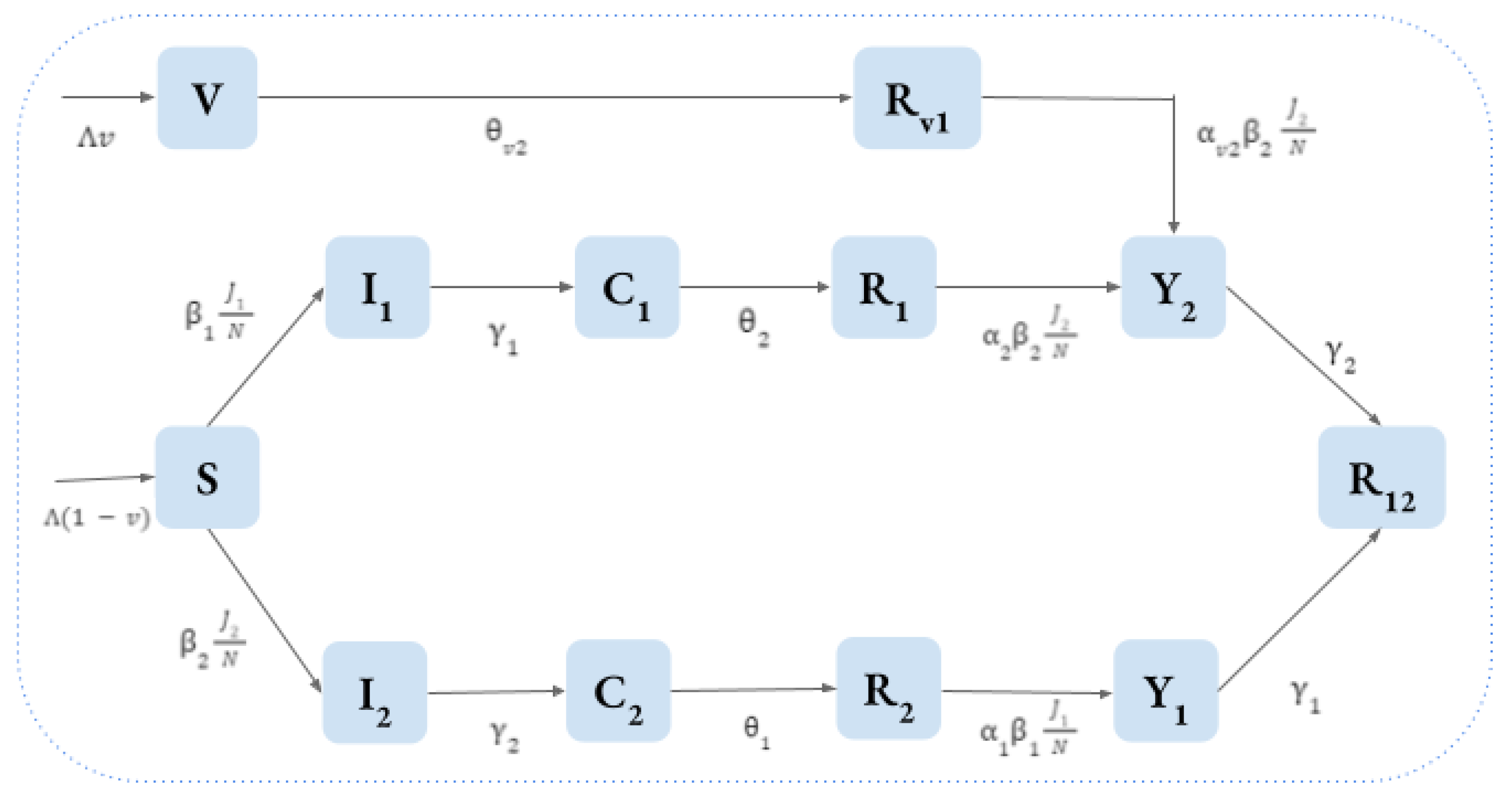
6.3. Effects of Single-Strain Vaccination on the Dynamics of a Multi-Strain Host-Only Dengue Model with ADE

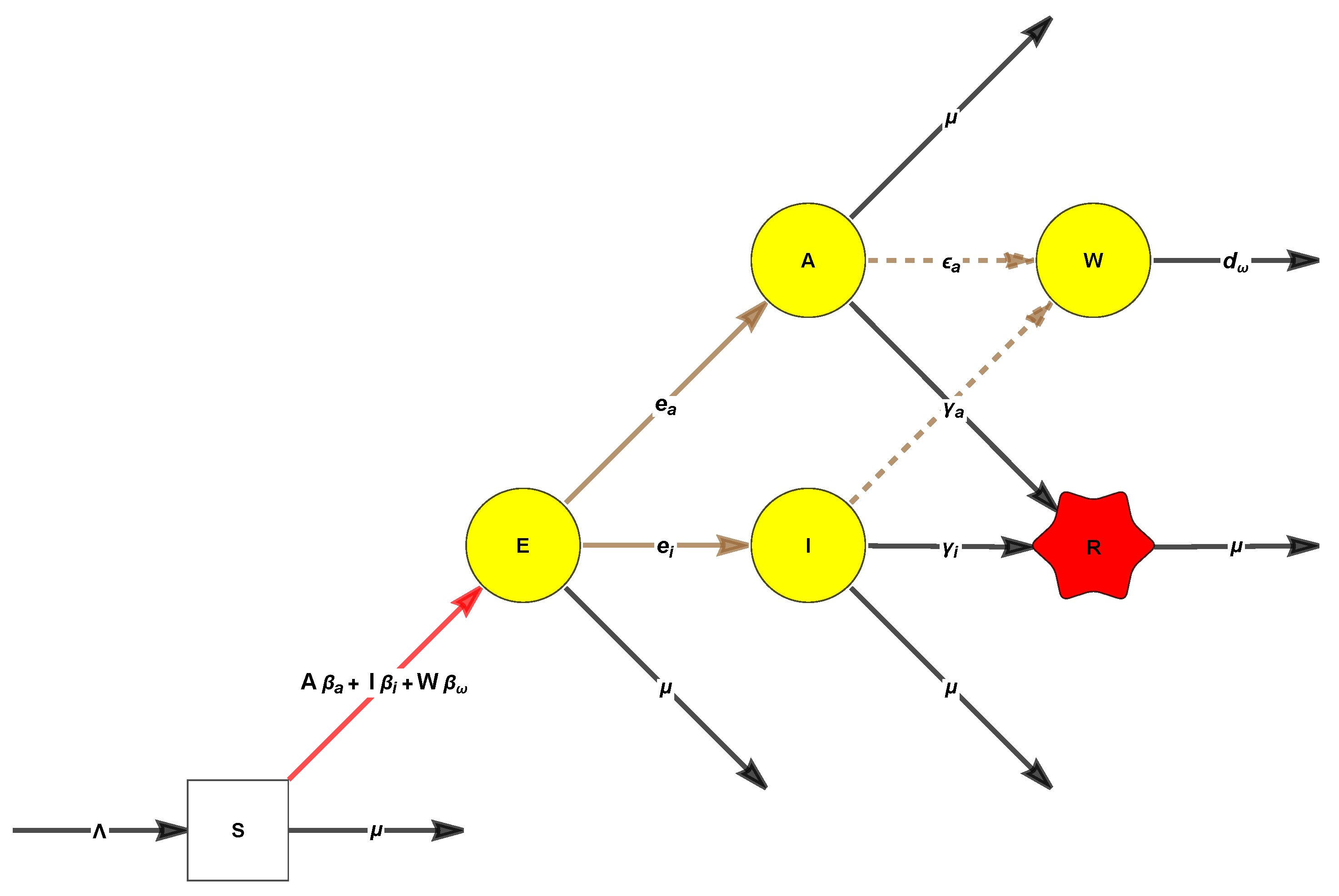
In this section, we will show that the mysterious Formula (34) continues to hold under the considerably more complicated two-strains model of [56], with vaccination applied to one strain only. The model studied in [56] is depicted in Figure 5.

This model involves twelve compartments, two of which capture the vaccination against strain 1.

1.

$S=S_0$ are individuals susceptible to both strains;

2.

$I_i$, for $i,j=1,2$ are individuals infected with strain i, with temporary cross-immunity to strain $j\ne i$;

3.

$C_i$ ($R_i$ in the original model of [52]) are individuals recovered from strain i, and hence, are permanently immune to it, with temporary cross-immunity to strain $j\ne i$;

4.

$R_i$ ($S_i$ in the original model of [52]) are unvaccinated individuals who have recovered from strain i, but have now become susceptible to the other strain j;

5.

$Y_j$ ($I_{ij}$ in the original model of [52]) are individuals previously infected with strain i and are immune to it, but have become reinfected with strain $j,i,j=1,2,i\ne j$;

6.

$R=R_{12}$ are individuals immune to all the strains;

7.

Finally, there are individuals V who are vaccinated against strain 1 and are still susceptible to strain 2, and individuals $R_{v1}=S_v=Z$ who have been vaccinated against strain 1 and have subsequently become infected by strain 2.

Denote by $N\left(t\right)=S\left(t\right)+V\left(t\right)+I_1\left(t\right)+I_2\left(t\right)+C_1\left(t\right)+C_2\left(t\right)+R_1\left(t\right)+R_2\left(t\right)+Y_1\left(t\right)+Y_2\left(t\right)+S_v\left(t\right)+R_{12}\left(t\right)$ the total population, put $J_i=I_i+Y_i,i=1,2$, and assume that the two forces of infection acting on S are:

$$F_i={\beta }_i\frac{J_i}{N},$$

and that the forces of infection acting on $Y_i=S_i,i=1,2$ are:

$${\alpha }_1{\beta }_1\frac{J_1}{N},{\alpha }_2{\beta }_2\frac{J_2}{N},{\alpha }_v{\beta }_2\frac{J_2}{N},$$

where ${\alpha }_1,{\alpha }_2,{\alpha }_v$ denote the decreases or increases in the susceptibility to secondary infections (${\alpha }_i>1$ implying an ADE effect).

The following equations, with appropriate initial conditions, represent the disease dynamics model:

$$\begin{array}{cc}\hfill {\displaystyle \frac{dS}{dt}}& =(1-\xi )\mu -{\beta }_1{J}_1\frac{S}{N}-{\beta }_2{J}_2\frac{S}{N}-\mu S\hfill \\ \hfill {\displaystyle \frac{d{I}_1}{dt}}& ={\beta }_1{J}_1\frac{S}{N}-({\gamma }_1+\mu )I_1\hfill \\ \hfill {\displaystyle \frac{d{C}_1}{dt}}& ={\gamma }_1{I}_1-({\theta }_1+\mu )C_1\hfill \\ \hfill {\displaystyle \frac{d{R}_1}{dt}}& ={\theta }_2{C}_1-{\alpha }_2{\beta }_2{J}_2\frac{R_1}{N}-\mu R_1\hfill \\ \hfill {\displaystyle \frac{d{Y}_2}{dt}}& ={\alpha }_2{\beta }_2{J}_2\frac{R_1}{N}+{\alpha }_v{\beta }_2{J}_2\frac{S_v}{N}-({\gamma }_2+\mu )Y_2\hfill \\ \hfill {\displaystyle \frac{d{I}_2}{dt}}& ={\beta }_2{J}_2\frac{S}{N}-({\gamma }_2+\mu )I_2\hfill \\ \hfill {\displaystyle \frac{d{C}_2}{dt}}& ={\gamma }_2{I}_2-({\theta }_2+\mu )C_2\hfill \\ \hfill {\displaystyle \frac{d{R}_2}{dt}}& ={\theta }_1{C}_2-{\alpha }_1{\beta }_1{J}_1\frac{R_2}{N}-\mu R_2\hfill \\ \hfill {\displaystyle \frac{d{Y}_1}{dt}}& ={\alpha }_1{\beta }_1{J}_1\frac{R_2}{N}-({\gamma }_1+\mu )Y_1\hfill \\ \hfill {\displaystyle \frac{dV}{dt}}& =\xi \mu -({\theta }_v+\mu )V\hfill \\ \hfill {\displaystyle \frac{d{S}_v}{dt}}& ={\theta }_{v}V-{\alpha }_v{\beta }_2{J}_2\frac{S_v}{N}-\mu S_v\hfill \\ \hfill {\displaystyle \frac{d{R}_{12}}{dt}}& ={\gamma }_1{Y}_1+{\gamma }_2{Y}_2-\mu R_{12}\hfill \end{array}$$

(36)

Table 1. Parameters and compartments of the model.

Parameter	Description (for $\mathit{i},\mathit{j}=1,2$)
$\mu$	Birth rate
$\mu$	Per capita death rate
${\beta }_i$	Transmission rate of virus i
${\gamma }_i$	Per capita recovery rate of infected people with virus i
${\theta }_i$	Per capita loss rate of cross-immunity to virus i after previous infection with virus j
${\theta }_v$	Per capita loss rate of cross-immunity to virus 2 obtained via vaccination
${\alpha }_i$	ADE factor that can alter the susceptibility of unvaccinated individuals to the virus i
${\alpha }_v$	ADE factor that can alter the susceptibility of vaccinated individuals to virus 2
$\xi$	Per capita vaccination rate
Compartments	Description
S	Susceptible individuals to both viruses
V	Vaccinated individuals against the virus 1
$I_i$	Individuals with primary infection by the virus i
$C_i$	Individuals recovered from infection with virus i and have cross-immunity to virus j
$R_i$	Unvaccinated individuals immune to virus i and susceptible to virus j
$Z=S_v$	Individuals vaccinated for virus 1, and susceptible to virus 2
$Y_1$	Individuals infected by virus 1 and recovered and hence, immune to virus 2
$Y_2$	Individuals infected by virus 2 and immune to virus 1 either due to recovery or vaccination
$R_{12}$	Individuals immune to both virus

summarizes the parameters and compartments of the model.

This system does not have negative cross effects; therefore, it leaves the non-negative quadrant invariant [57]. It follows from the equations that

$$\frac{dN\left(t\right)}{dt}=\mu (1-N\left(t\right)).$$

Therefore,

$$\underset{t\to +\infty }{lim}N\left(t\right)=1.$$

Assuming $N\left(0\right)=1$ implies that $N\left(t\right)=1$, for $t\ge 0$. Using this, we may assume w.l.o.g. that $N=1$, working with the proportions, is to be denoted by the corresponding lowercase letters.

The only non-zero compartments in the DFE, to be denoted by $E_0$, are easily found to be

$$s_0=1-\xi ,z_0=\xi \frac{{\theta }_v}{\mu +{\theta }_v},v_0=\xi \frac{\mu }{\mu +{\theta }_v};$$

in fact, the last value holds at any fixed point. As known from [56], there are also two endemic points on the boundary, whose rather complicated formulas will be given later.

Remark 21. 

From a modeling point of view, this system has crucial parameters like ${\alpha }_v$ (note that ${\alpha }_v=0$ means perfect vaccination, and ${\alpha }_v=1$, which means that infection by the second strain is equally likely for vaccinated people).

Due to conservation, the system evolves in a compact domain, and so we may eliminate one compartment, for example, V, from the analysis. Finally, the last compartment does not send input to the others and therefore may also be disregarded in the analysis.

6.3.1. The Jacobian $R_J\left(X\right)$ Is the Max of Two Polynomials, Obtained Using a Minimal Disease Set

We may tackle this example via the Jacobian factorization approach, choosing the minimal disease set $\mathcal{I}=(i_1,i_2,y_1,y_2)$, just like in the previous section. Again, the characteristic polynomial of the Jacobian with the variables in $\mathcal{I}$ are set to 0 factors completely as a product of the linear terms

$${(\mu +u)}^5\left({\gamma }_1+\mu +u\right)\left({\gamma }_2+\mu +u\right)\left({\theta }_1+\mu +u\right)\left({\theta }_2+\mu +u\right)\left(\mu +u+{\theta }_v\right)\times$$

$$\begin{array}{c}\hfill \left({\gamma }_1+\mu -{\alpha }_1{\beta }_1{r}_2-{\beta }_{1}s+u\right)\left({\gamma }_2+\mu -{\alpha }_2{\beta }_2{r}_1-{\beta }_{2}s-{\beta }_{2}z{\alpha }_v+u\right),\end{array}$$

only two of which (the seventh and eighth factors) may yield positive eigenvalues. Both are of the Descartes type, and instability may occur if

$$R_J\left(X\right):=max[R_1\left(X\right),R_2\left(X\right)]=max[\frac{{\beta }_1\left({\alpha }_1{r}_2+s\right)}{{\gamma }_1+\mu },\frac{{\beta }_2\left({\alpha }_2{r}_1+z{\alpha }_v+s\right)}{{\gamma }_2+\mu }]>1.$$

(37)

At the DFE, $r_1=r_2=0,$ and this yields

$$R_J:=R_J\left(E_0\right)=R_N=max[s_0\frac{{\beta }_1}{d_1},s_0\frac{{\beta }_2}{d_2}+z_0\frac{{\beta }_2{\alpha }_v}{d_2}],d_1={\gamma }_1+\mu ,d_2={\gamma }_2+\mu .$$

(38)

This expression reveals a pattern similar to (16), with the difference that the existence of two strains are reflected in the max and that the second strain is alimented by two classes of susceptibles, one of which is the people vaccinated against the first strain.

In addition to the disease-free equilibrium, there might exist two more equilibriums on the boundary: the endemic equilibrium where there are only infections by strain 1, $E_1$, and the endemic equilibrium where there are only infections by strain 2, $E_2$; this will be reviewed in the next section.

6.3.2. The Endemic Boundary Equilibrium $E_i$ Exist If $R_i\left(E_0\right)>1$

At the equilibrium $E_1$, the values of $I_2,C_2,R_2,Y_1,Y_2$ and $R_{12}$ are zero. The coordinates are easily found using the “Solve” command. Those of $V,Z$ are the same as at the DFE, and the others are:

$$\begin{array}{c}\hfill s_1=\frac{{\gamma }_1+\mu }{{\beta }_1},i_1=\frac{\mu }{{\beta }_1}\left[\frac{1-\xi }{s_1}-1\right]:=\frac{\mu }{{\beta }_1}\left({\mathcal{R}}_1-1\right),c_1=\frac{{\gamma }_1}{{\theta }_1+\mu }{i}_1,r_1=\frac{{\theta }_1}{\mu }{c}_1\end{array}$$

(39)

where

$${\mathcal{R}}_1=(1-\xi )\frac{{\beta }_1}{{\gamma }_1+\mu }=R_1\left(E_0\right)$$

(40)

(the endemic equilibrium $E_1$ exists if and only if ${\mathcal{R}}_1>1$).

At the equilibrium $E_2$, the values of $I_1,C_1,R_1$ and $Y_1$ are zero, and that of V is the same as at the DFE.

The solutions of the $E_2$ system involve all complicated square roots. In such a case, it is more convenient to replace the “Solve” command by our RUR algorithm, which requires the user to input a variable to reduce 2. The normal choice is $i_2$ (which transitions to positive at the bifurcation value), but here we will use s, to check the results of [56], who find, using as a reduction scalar $x={\beta }_2{j}_2,$ that

$$\begin{array}{ccc}\hfill & & s_2=\frac{(1-\xi )\mu }{x+\mu },i_2=\frac{(1-\xi )x\mu }{(x+\mu )({\gamma }_2+\mu )},c_2=\frac{(1-\xi )x{\gamma }_2\mu }{(x+\mu )({\gamma }_2+\mu )({\theta }_1+\mu )},\hfill \\ & & r_2=\frac{(1-\xi )x{\gamma }_2{\theta }_1}{(x+\mu )({\gamma }_2+\mu )({\theta }_1+\mu )},z_2=\frac{v{\theta }_v\mu }{({\theta }_v+\mu )({\alpha }_{v}x+\mu )},\hfill \\ & & y_2=\frac{v{\alpha }_{v}x{\theta }_v\mu }{({\alpha }_{v}x+\mu )({\theta }_v+\mu )({\gamma }_2+\mu )},\hfill \end{array}$$

(41)

and that x is the solution of the quadratic equation

$$a{x}^2+bx+c=0,\left\{\begin{array}{cc}a\hfill & ={\alpha }_v\hfill \\ b\hfill & =\mu {\alpha }_v\left[1-\frac{{\beta }_2(1-\xi )}{{\gamma }_2+\mu }\right]+\mu \left[1-\frac{{\beta }_2{\alpha }_v{\theta }_{v}v}{({\gamma }_2+\mu )({\theta }_v+\mu )}\right]\hfill \\ c\hfill & ={\mu }^2\left(1-{\mathcal{R}}_2\right)\hfill \end{array}\right..$$

The equilibrium $E_2$ exists if ${\mathcal{R}}_2>1$, where

$${\mathcal{R}}_2=\frac{{\beta }_2}{{\gamma }_2+\mu }\left[1-\xi +\xi \frac{{\alpha }_v{\theta }_v}{{\theta }_v+\mu }\right]=\frac{{\beta }_2}{{\gamma }_2+\mu }\left[s_0+{\alpha }_v{z}_0\right]=R_2\left(E_0\right).$$

(42)

If ${\mathcal{R}}_2\le 1$, the fractions in the expression of b must be smaller than one or equal to one, and it is not possible for both to be one. Therefore, $b>0$. We also have $c\ge 0$. Since that $a>0$, Equation (42) does not have roots with positive real parts. This implies that there is no endemic equilibrium like $E_2$. Thus, in this case, $c<0$. Since the coefficient a is positive, Equation (42) has two real roots and only one of them is positive. To resume, if ${\mathcal{R}}_2>1$, there is a unique endemic equilibrium where there are infections only by strain 2.

6.3.3. The Recipe next-generation matrix $R_0$ and the Jacobian Factorization One Coincide

This section shows that the polynomials $R_1\left(X\right),R_2\left(X\right)$ in this example may also be obtained via the next-generation matrix approach as eigenvalues of the K matrix via a judicious choice of infectious classes.

One may choose, as the infectious subset, the nine compartments that are 0 in the limit, but a luckier choice here is the smaller subset $\mathcal{I}=\{I_1,I_2,Y_2,Y_1\}$, which precisely has, as eigenvalues, the expressions $R_1\left(X\right),R_2\left(X\right)$ in (33).

The decomposition matrices are

$$V=\left(\begin{array}{cccc}{\gamma }_1+\mu & 0& 0& 0\\ 0& {\gamma }_2+\mu & 0& 0\\ 0& 0& {\gamma }_1+\mu & 0\\ 0& 0& 0& {\gamma }_2+\mu \end{array}\right),F=\left(\begin{array}{cccc}{\beta }_{1}s& 0& 0& {\beta }_{1}s\\ 0& {\beta }_{2}s& {\beta }_{2}s& 0\\ 0& {\beta }_{2}z{\alpha }_v& {\beta }_2\zeta {\alpha }_v& 0\\ 0& 0& 0& 0\end{array}\right)=s{B}_0+z{B}_v,$$

where $B_0,B_v$ are:

$$\begin{array}{c}\hfill B_0=\left(\begin{array}{cccc}{\beta }_1& 0& 0& {\beta }_1\\ 0& {\beta }_2& {\beta }_2& 0\\ 0& 0& 0& 0\\ 0& 0& 0& 0\end{array}\right),B_v=\left(\begin{array}{cccc}0& 0& 0& 0\\ 0& 0& 0& 0\\ 0& {\beta }_2{\alpha }_v& {\beta }_2{\alpha }_v& 0\\ 0& 0& 0& 0\end{array}\right).\end{array}$$

The explicit non-zero eigenvalues of the next-generation matrix $(\mathsf{s}{B}_0+z{B}_v)V^{-1}$ are

$$\left(\frac{{\beta }_1\mathsf{s}}{{\gamma }_1+\mu },\frac{{\beta }_2\left(z{\alpha }_v+\mathsf{s}\right)}{{\gamma }_2+\mu }\right),$$

(43)

confirming the result of the Jacobian method.

Let us note finally that (37), as well as the result of this section, imply the relation

$$R_0=max\left[{\mathcal{R}}_1,{\mathcal{R}}_2\right],$$

(44)

where ${\mathcal{R}}_i,i=1,2$ denote the bifurcation parameters at which the boundary points $E_i$ start to exist.

Remark 22. 

Interestingly, $R_0=max[{\mathcal{R}}_1,{\mathcal{R}}_2]$ is the max of two quantities which satisfy that ${\mathcal{R}}_i>1,i=1,2$ are precisely the domains where endemic points $E_i$ containing exactly one of the strains appear—see (44). This formula, natural in cases where the next-generation matrix has a block structure, seems to be a general feature of multi-strain models, even when the block structure is not apparent.

In the case of this section, there seems to be a more specific structure: the Jacobian factorization approach allows for introducing two “Descartes type” (see Definition 1) factors $R_i\left(X\right),i=1,2$ of the characteristic polynomial, which are that

1.

The existence conditions for$E_i$may be expressed as${\mathcal{R}}_i:=R_i\left(DFE\right)>1$—see (40), (42), and (46).

2.

The invasion reproduction numbers may be obtained simply by substituting the coordinates of the dominance boundary equilibria into the corresponding factor. More precisely, the invasion number of the fixed point $E_i$ for strain i is given by $R_{ji}=R_j\left(E_i\right)$.

Open question 2: Does the relation $R_0={max}_1^K{\mathcal{R}}_k$ hold for all Descartes multi-strain models of order K? (recall Definition 3 and Lemma 3).

6.3.4. The Invasion Reproduction Number of $E_i$ Is Given by $R_j\left(E_i\right)$

The invasion reproduction numbers (see for example [58]) may, just as the basic reproduction number, be calculated using the next-generation matrix.

Our script yields quickly that

$${\mathcal{R}}_{ji}=R_j\left(E_i\right),i=1,2,j\ne i.$$

(45)

Open question 3: Do the formulas connecting (44) and (45) to the Jacobian factorization

$$\left\{\begin{array}{c}{\mathcal{R}}_i=R_i\left(E_0\right),R_0=max\left[{\mathcal{R}}_1,{\mathcal{R}}_2\right],\hfill \\ {\mathcal{R}}_{ji}=R_j\left(E_i\right),\mathrm{where}{R}_i\mathrm{denote}\mathrm{polynomials}\mathrm{obtained}\mathrm{via}\hfill \\ \mathrm{the}\mathrm{Jacobian}\mathrm{factorization}\mathrm{approach},\hfill \end{array}\right.$$

(46)

hold for some general class of epidemic models?

(C) For “two strain epidemic models”, what conditions must be satisfied to ensure the inequalities ${\mathcal{R}}_{ji}<{\mathcal{R}}_j,i=1,2,j\ne i$?

To resolve these questions, it might be useful to study the three and four strain generalizations of this problem and to investigate “non-simple” multi-strain models (in which the characteristic polynomial contains non-Descartes type polynomials).

7. Vector–Host Models

7.1. The Jacobian $R_0$ Is the Square of the Recipe NGM $R_0$ for the Dengue Vector–Host Model without Demography of [30]

Ref. ([30] eq(28)) considers a “no demography/conservation” model with six compartments, three of which represent hosts, while the rest represent the vector. Note that such models with no demography do not have a finite set of fixed points. The DFE is not unique, it coincides with the initial conditions. However, our algorithm works just fine. The model, after removing two “R” classes which do not affect the rest, is:

$$\left\{\begin{array}{c}{S}_1^{\prime }=-\frac{{\beta }_{21}{I}_2{S}_1}{N_1}\hfill \\ S_2^{\prime }=-\frac{{\beta }_{12}{I}_1{S}_2}{N_2}\hfill \\ \left(\begin{array}{c}{I}_1^{\prime }\\ I_2^{\prime }\end{array}\right)=\left(\begin{array}{cc}-{\gamma }_1& \frac{{\beta }_{21}{S}_1}{N_1}\\ \frac{{\beta }_{12}{S}_2}{N_2}& -{\gamma }_2\end{array}\right)\left(\begin{array}{c}{I}_1\\ I_2\end{array}\right)\hfill \end{array}\right..$$

(47)

The call “$\inf =\{1,2\}; NGM[Brouwer22,\inf ]$” of our script yields that the decomposition matrices are

$$F=\left(\begin{array}{cc}0& \frac{{\beta }_{21}{S}_1}{N_1}\\ \frac{{\beta }_{12}{S}_2}{N_2}& 0\end{array}\right),V=\left(\begin{array}{cc}{\gamma }_1& 0\\ 0& {\gamma }_2\end{array}\right),$$

$$K=\left(\begin{array}{cc}0& \frac{{\beta }_{21}{S}_1}{{\gamma }_2{N}_1}\\ \frac{{\beta }_{12}{S}_2}{{\gamma }_1{N}_2}& 0\end{array}\right),$$

and

$$R_F=\sqrt{\frac{S_1{S}_2{\beta }_{12}{\beta }_{21}}{N_1{N}_2{\gamma }_1{\gamma }_2}}.$$

(48)

After using the fact that the DFE is determined by the initial conditions $S_1=N_1$, and $S_2=N_2$, we obtain the basic reproduction number

$$R_F=\sqrt{\frac{{\beta }_{12}{\beta }_{21}}{{\gamma }_1{\gamma }_2}}$$

(49)

of ([30] eq(40)).

Here the characteristic polynomial is of the Descartes type and the Jacobian method, as well as the RUR method, yielding for both the square of the (modified) formula (48) $R_J=\frac{{\beta }_{12}{\beta }_{21}}{{\gamma }_1{\gamma }_2}$.

Remark 23. 

Note that ([30] eq(35)) offers yet another admissible decomposition, based on a different biological interpretation, with $R_F=R_J$, and raises the question of which of the answers is more relevant for a given epidemic. Deciding this from the ODE model only seems impossible.

7.2. The Two Groups Model in ([21] eq(5.8)) Does Not Obey a Square Relation

The two groups model in ([21] eq(5.8)) defined by

$$\begin{array}{c}\hfill \left\{\begin{array}{c}{S}_1^{\prime }=-\frac{{\beta }_{11}{I}_1{S}_1}{N_1}-\frac{{\beta }_{21}{I}_2{S}_1}{N_1}+{\lambda }_1-{\mu }_1{S}_1\hfill \\ S_2^{\prime }=-\frac{{\beta }_{12}{I}_1{S}_2}{N_2}-\frac{{\beta }_{22}{I}_2{S}_2}{N_2}+{\lambda }_2-{\mu }_2{S}_2\hfill \\ \left(\begin{array}{c}{I}_1^{\prime }\\ I_2^{\prime }\end{array}\right)=\left(\begin{array}{cc}-{\gamma }_1-{\mu }_1-{\delta }_1+\frac{{\beta }_{11}{S}_1}{N_1}& \frac{{\beta }_{21}{S}_1}{N_1}\\ \frac{{\beta }_{12}{S}_2}{N_2}& \frac{{\beta }_{22}{S}_2}{N_2}-{\gamma }_2-{\mu }_2-{\delta }_2\end{array}\right)\left(\begin{array}{c}{I}_1\\ I_2\end{array}\right)\hfill \end{array}\right.\end{array}$$

is not a vector–host model anymore, due to the addition of the “intra-group contact infection rates” ${\beta }_{11},{\beta }_{22}$.

The DFE is $\left\{0,0,\frac{{\lambda }_1}{{\mu }_1},\frac{{\lambda }_2}{{\mu }_2}\right\}$, and the $R_N$ is quite complicated:

$$\begin{array}{ccc}& & \frac{\sqrt{\left({\beta }_{22}{N}_1{S}_2\left({\gamma }_1+{\delta }_1+{\mu }_1\right)+{\beta }_{11}{N}_2{S}_1\left({\gamma }_2+{\delta }_2+{\mu }_2\right)\right){}^2+4\left({\beta }_{12}{\beta }_{21}-{\beta }_{11}{\beta }_{22}\right)N_1{N}_2{S}_1{S}_2\left({\gamma }_1+{\delta }_1+{\mu }_1\right)\left({\gamma }_2+{\delta }_2+{\mu }_2\right)}}{2N_1{N}_2\left({\gamma }_1+{\delta }_1+{\mu }_1\right)\left({\gamma }_2+{\delta }_2+{\mu }_2\right)}\hfill \\ & & +\frac{{\beta }_{22}{\gamma }_1{N}_1{S}_2+{\beta }_{11}{\gamma }_2{N}_2{S}_1+{\beta }_{22}{\delta }_1{N}_1{S}_2+{\beta }_{11}{\delta }_2{N}_2{S}_1+{\beta }_{22}{\mu }_1{N}_1{S}_2+{\beta }_{11}{\mu }_2{N}_2{S}_1}{2N_1{N}_2\left({\gamma }_1+{\delta }_1+{\mu }_1\right)\left({\gamma }_2+{\delta }_2+{\mu }_2\right)}.\hfill \end{array}$$

(50)

The Jacobian factorization method yields a different answer for a characteristic polynomial which is not of the Descartes type, precisely because of the addition of ${\beta }_{11},{\beta }_{22}$.

$$R_J=\frac{{\beta }_{22}{N}_1{S}_2\left({\gamma }_1+{\delta }_1+{\mu }_1\right)+{\beta }_{11}{\gamma }_2{N}_2{S}_1+{\beta }_{11}{\delta }_2{N}_2{S}_1+{\beta }_{11}{\mu }_2{N}_2{S}_1+{\beta }_{12}{\beta }_{21}{S}_1{S}_2}{N_1{N}_2\left({\gamma }_1+{\delta }_1+{\mu }_1\right)\left({\gamma }_2+{\delta }_2+{\mu }_2\right)+{\beta }_{11}{\beta }_{22}{S}_1{S}_2}.$$

8. Multi-Strain Vector–Host Models

8.1. A Two-Strain Vector–Host Model of Feng and Velasco-Hernández [59], Where the Square Relation Holds for the Basic Reproduction Number

Ref. [59] considered a human population settled in a region where a mosquito population of the genus Aedes is present and is a carrier of two strains of the dengue virus. Let $V_i,I_i,Y_i,i=1,2$ denote the infected mosquitoes, individuals infected by one strain, and individuals having suffered a secondary infection, respectively, let $N=S+R+{\sum }_{i=1}^2{I}_i+Y_i$ denote the total human population, and let $B_1=\frac{{\beta }_1{V}_1\left(t\right)}{c+w_{h}N},B_2=\frac{{\beta }_2{V}_2\left(t\right)}{c+w_{h}N}$ denote the rates of infections in human hosts produced by the two strains. The model is defined as follows:

$$\begin{array}{c}\hfill \left\{\begin{array}{c}{S}^{\prime }\left(t\right)=h-S\left(t\right)\left(B_1+B_2\right)-\mu S\left(t\right),\hfill \\ I_1^{\prime }\left(t\right)=B_{1}S\left(t\right)-{\sigma }_2{B}_2{I}_1\left(t\right)-\mu I_1\left(t\right),\hfill \\ I_2^{\prime }\left(t\right)=B_{2}S\left(t\right)-{\sigma }_1{B}_1{I}_2\left(t\right)-\mu I_2\left(t\right),\hfill \\ Y_1^{\prime }\left(t\right)={\sigma }_1{B}_1{I}_2\left(t\right)-(e_1+\mu +r)Y_1\left(t\right),\hfill \\ Y_2^{\prime }\left(t\right)={\sigma }_2{B}_2{I}_1\left(t\right)-(e_2+\mu +r)Y_2\left(t\right),\hfill \\ R^{\prime }\left(t\right)=r(Y_1\left(t\right)+Y_2\left(t\right))-\mu R\left(t\right),\hfill \\ \\ V_1^{\prime }\left(t\right)={\alpha }_1\frac{I_1\left(t\right)+Y_1\left(t\right)}{c+w_{v}N}M\left(t\right)-\delta V_1\left(t\right),\hfill \\ V_2^{\prime }\left(t\right)={\alpha }_2\frac{I_2\left(t\right)+Y_2\left(t\right)}{c+w_{v}N}M\left(t\right)-\delta V_2\left(t\right)\hfill \\ M^{\prime }\left(t\right)=q-M\left(t\right)\left({\alpha }_1\frac{I_1\left(t\right)+Y_1\left(t\right)}{c+w_{v}N}+{\alpha }_2\frac{I_2\left(t\right)+Y_2\left(t\right)}{c+w_{v}N}\right)-\delta M\left(t\right).\hfill \end{array}\right.\end{array}$$

The DFE is given by $E_0=\left(h/\mu ,0,0,0,0,0,0,0,q/\delta \right)$. For the infectious set $I_1,I_2,Y_1,Y_2,V_1,V_2$, the F and V matrices used in the next-generation approach are given by

$$\begin{array}{ccc}& & F=\left(\begin{array}{cccccc}0& 0& 0& 0& {\beta }_1{s}_{dfe}& 0\\ 0& 0& 0& 0& 0& {\beta }_2{s}_{dfe}\\ 0& 0& 0& 0& 0& 0\\ 0& 0& 0& 0& 0& 0\\ {\alpha }_1{M}_{dfe}& 0& {\alpha }_1{M}_{dfe}& 0& 0& 0\\ 0& {\alpha }_2{M}_{dfe}& 0& {\alpha }_2{M}_{dfe}& 0& 0\end{array}\right),\hfill \end{array}$$

(51)

$$\begin{array}{ccc}& & V=\left(\begin{array}{cccccc}\mu & 0& 0& 0& 0& 0\\ 0& \mu & 0& 0& 0& 0\\ 0& 0& e_1+r+\mu & 0& 0& 0\\ 0& 0& 0& e_2+r+\mu & 0& 0\\ 0& 0& 0& 0& \delta & 0\\ 0& 0& 0& 0& 0& \delta \end{array}\right)\hfill \end{array}$$

(52)

with $M_{dfe}=q/\delta$. Then,

$$F{V}^{-1}=\left(\begin{array}{cccccc}0& 0& 0& 0& \frac{{\beta }_1{s}_{dfe}}{\delta }& 0\\ 0& 0& 0& 0& 0& \frac{{\beta }_2{s}_{dfe}}{\delta }\\ 0& 0& 0& 0& 0& 0\\ 0& 0& 0& 0& 0& 0\\ \frac{{\alpha }_1{M}_{dfe}}{\mu }& 0& \frac{{\alpha }_1{M}_{dfe}}{e_1+\mu +\xi }& 0& 0& 0\\ 0& \frac{{\alpha }_2{M}_{dfe}}{\mu }& 0& \frac{{\alpha }_2{M}_{dfe}}{e_2+\mu +\xi }& 0& 0\end{array}\right)$$

We obtain a basic reproduction number, which is a max

$$\mathcal{R}=max\left(\sqrt{{\mathcal{R}}_1},\sqrt{{\mathcal{R}}_2}\right),{\mathcal{R}}_i:=s_0{m}_0\frac{{\alpha }_i{\beta }_i}{\delta \mu },$$

(53)

just like (44), but also contains the extra square roots typical of vector–host models.

Furthermore, it may be checked that this is precisely the square root of the answer given by the Jacobian factorization method, which decomposes the characteristic polynomial of the Jacobian as the product of five linear factors with negative roots and two quadratic Descartes type polynomials.

There also two boundary (dominance) equilibria where only one strain survives. The non-zero coordinates at the first one, $E_1$, are given by

$${\alpha }_1{i}_1=\delta \frac{{\mathcal{R}}_1-1}{m_0{\beta }_1/\left(\mu \right)+1},{\beta }_1{v}_1=\mu \frac{{\mathcal{R}}_1-1}{s_0{\alpha }_1\left(\delta \right)+1},s=\mu \frac{{\alpha }_1{s}_0+\delta }{{\alpha }_1{\beta }_1{m}_0+{\alpha }_1\mu },$$

with similar formulas holding for the other boundary point $E_2$, using symmetry. Thus, these points become positive precisely when the corresponding factor of the DFE becomes bigger than 1, causing instability.

Since we had trouble with computing the invasion reproduction numbers, we switched to the “simplified model” of [59], in which M is eliminated by noting that the equation for the total vector population $T=M+V_1+V_2$ is $T^{\prime }=q-\delta T$, and also by assuming that $T_0={lim}_{t\to \infty }T\left(t\right)=q/\delta$, M can be removed from the system by substituting

$$M=q/\delta -V_1-V_2.$$

(54)

As a first consequence of using (54), the $R_N$ becomes equal to $R_J$.

However, the recipe $R_0$ at $E_1$ for the natural choice of “inf” is very complicated, and [59] provides here a laborious local stability analysis, with a complicated result, via the third-order Routh–Hurwitz conditions.

We note finally that the characteristic polynomial for $jac\left(E_1\right)$ has two factors of degree 3, one of which is the Descartes type, and one which is not. The Descartes type factor yields a polynomial $R_1\left(X\right)$. Putting this together with its symmetric $R_2\left(X\right)$ allows us to finally define

$$R_J\left(X\right)=ma{x}_j[R_1\left(X\right),R_2\left(X\right)]=ma{x}_j\left[\frac{{\alpha }_j{\beta }_{j}qs/\delta }{({\beta }_j{v}_j+\mu )\left({\alpha }_j{i}_j+\delta \right)+{\beta }_j{v}_j{\alpha }_{j}s}\right].$$

Invasion Numbers of [59]

The two-strain vector–host model in [59] admits two boundary equilibria beside the DFE in which

$S_1^{*},S_2^{*},I_1^{*},I_2^{*},V_1^{*},V_2^{*}$ are the invasion infection classes. In this case, we consider the subset ${\mathrm{in}}_1=\left(I_2,Y_1,Y_2,V_2\right)$ corresponding to the invasion infection class of $E_1$, then

$$F=\left(\begin{array}{cccc}0& 0& 0& b_{2}S\\ b_1{\sigma }_1{v}_1& 0& 0& 0\\ 0& 0& 0& b_2{i}_1{\sigma }_2\\ a_2\left(\frac{q}{\delta }-v_1\right)& 0& a_2\left(\frac{q}{\delta }-V_1\right)& 0\end{array}\right),$$

(55)

$$V=\left(\begin{array}{cccc}{b}_1{\sigma }_1{V}_1+\mu & 0& 0& 0\\ 0& e_1+\mu +\xi & 0& 0\\ 0& 0& e_2+\mu +\xi & 0\\ a_2\left(\frac{q}{\delta }-V_1\right)-a_2\left(\frac{q}{\delta }-V_1-V_2\right)& 0& a_2\left(\frac{q}{\delta }-V_1\right)-a_2\left(\frac{q}{\delta }-V_1-V_2\right)& a_2\left(I_2+Y_2\right)+\delta \end{array}\right),$$

(56)

$$K=\left(\begin{array}{cccc}0& 0& 0& \frac{b_{2}S}{\delta }\\ \frac{b_1{\sigma }_1{V}_1}{b_1{\sigma }_1{V}_1+\mu }& 0& 0& 0\\ 0& 0& 0& \frac{b_2{I}_1{\sigma }_2}{\delta }\\ \frac{a_2\left(\frac{q}{\delta }-V_1\right)}{b_1{\sigma }_1{V}_1+\mu }& 0& \frac{a_2\left(\frac{q}{\delta }-V_1\right)}{e_2+\mu +\xi }& 0\end{array}\right)$$

then the IRN of strain 1 at $E_1$ is

$$R_1=\frac{\sqrt{a_2}\sqrt{b_2}\sqrt{q}\sqrt{S\left(e_2+\mu +\xi \right)}}{\delta \sqrt{\mu }\sqrt{e_2+\mu +\xi }}.$$

Similarly, we chose the other subset ${\mathrm{in}}_1=\left(I_1,Y_1,Y_2,V_1\right)$ corresponding to the invasion infection class at $E_2$, where we obtain

$$F=\left(\begin{array}{cccc}0& 0& 0& b_{1}S\\ 0& 0& 0& b_1{I}_2{\sigma }_1\\ b_2{\sigma }_2{V}_2& 0& 0& 0\\ a_1\left(\frac{q}{\delta }-V_2\right)& a_1\left(\frac{q}{\delta }-V_2\right)& 0& 0\end{array}\right),$$

(57)

$$V=\left(\begin{array}{cccc}{b}_2{\sigma }_2{V}_2+\mu & 0& 0& 0\\ 0& e_1+\mu +\xi & 0& 0\\ 0& 0& e_2+\mu +\xi & 0\\ a_1\left(\frac{q}{\delta }-V_2\right)-a_1\left(\frac{q}{\delta }-V_1-V_2\right)& a_1\left(\frac{q}{\delta }-V_2\right)-a_1\left(\frac{q}{\delta }-V_1-V_2\right)& 0& a_1\left(I_1+Y_1\right)+\delta \end{array}\right),$$

(58)

$$K=\left(\begin{array}{cccc}0& 0& 0& \frac{b_{1}S}{\delta }\\ 0& 0& 0& \frac{b_1{I}_2{\sigma }_1}{\delta }\\ \frac{b_2{\sigma }_2{V}_2}{b_2{\sigma }_2{V}_2+\mu }& 0& 0& 0\\ \frac{a_1\left(\frac{q}{\delta }-V_2\right)}{b_2{\sigma }_2{V}_2+\mu }& \frac{a_1\left(\frac{q}{\delta }-V_2\right)}{e_1+\mu +\xi }& 0& 0\end{array}\right)$$

then the maximum eigenvalue of K yields the IRN at $E_2$ which is

$$R_2=\frac{\sqrt{a_1}\sqrt{b_1}\sqrt{q-\delta v_2}\sqrt{I_2{\sigma }_1\left(b_2{\sigma }_2{V}_2+\mu \right)+e_{1}S+S(\mu +\xi )}}{\delta \sqrt{e_1+\mu +\xi }\sqrt{b_2{\sigma }_2{V}_2+\mu }}.$$

8.2. The Dengue–Zika Model with Coinfection and ADE [2]

The model studied in this paper continues previous papers like Isea and Lonngren 2016 [60] and Okuneye et al. 2017 [61], most notably by taking into account the possibility of coinfection and of direct transmission of Zika via sex (which entails two forces of infection for Zika transmissions in their flowchart, hence leading to an asymmetry in the results).

Introduce the following forces of infection:

$$\left\{\begin{array}{cc}{F}_{vd}={\beta }_{hd}{T}_{vd},T_{vd}=I_{vd}+I_{vc}{\nu }_d,\hfill & \mathrm{dengue}\mathrm{vector}\mathrm{force}\hfill \\ F_{vz}={\beta }_{hz}{T}_{vz},T_{vz}=I_{vz}+I_{vc}{\nu }_z,\hfill & \mathrm{zika}\mathrm{vector}\mathrm{force}\hfill \\ F_{hz}={\beta }_{vz}{T}_{hz},T_{hz}=I_z+I_c+J_z{k}_z,\hfill & \mathrm{zika}\mathrm{human}\mathrm{force}\hfill \\ F_{hd}={\beta }_{vd}{T}_{hd},T_{hd}=I_d+I_c+J_d{k}_d,\hfill & \mathrm{dengue}\mathrm{human}\mathrm{force}\hfill \\ F_s={\beta }_s{T}_{hz}\hfill & \mathrm{zika}\mathrm{human}\text{-}\mathrm{to}\text{-}\mathrm{human}\mathrm{force}.\hfill \end{array}\right.$$

(59)

Note that ${\nu }_d,{\nu }_z$ and $k_d,k_z$ are, respectively, the parameters of altered infectivity for co-infected vectors and of ADE, and note that even when ${\nu }_d={\nu }_z=1$, the co-infection model is more accurate than previous works like [59], since it takes into account the existence of doubly infected vectors $I_{vc}$ which influence both chains of infection.

We will consider the model:

$$\left\{\begin{array}{c}{S}_h^{\prime }=(N_h-S_h)\mu -S_h\left(F_{vd}+F_{vz}+F_s\right),\hfill \\ I_d^{\prime }=S_h{F}_{vd}-\rho I_d\left(F_{vz}+F_s\right)-I_d\left({\gamma }_d+\mu \right),\hfill \\ I_z^{\prime }=S_h(F_{vz}+F_s)-\rho I_z{F}_{vd}-I_z\left({\gamma }_d+\mu \right),\hfill \\ I_c^{\prime }=\rho \left[I_d\left(F_{vz}+F_s\right)+I_z{F}_{vd}-I_c\left({\gamma }_d+{\gamma }_c\right)\right]-\mu I_c,\hfill \\ R_d^{\prime }=I_d{\gamma }_d-R_d\left(F_{vz}+F_s+\mu \right),\hfill \\ R_z^{\prime }=I_z{\gamma }_d-R_z\left(F_{vd}+\mu \right),\hfill \\ J_d^{\prime }=\rho {\gamma }_z{I}_c+R_z\left(F_{vd}-{\gamma }_d-\mu \right),\hfill \\ J_z^{\prime }=\rho {\gamma }_d{I}_c+R_d\left(F_{vz}+F_s-{\gamma }_z-\mu \right),\hfill \\ R^{\prime }=J_d{\gamma }_d+J_z{\gamma }_z-\mu R,\hfill \\ S_v^{\prime }=(N_v-S_v){\mu }_v-S_v(F_{hd}+T_{hz}),\hfill \\ I_{vd}^{\prime }=F_{hd}{S}_v-\rho F_{hz}{I}_{vd}-I_{vd}{\mu }_v,\hfill \\ I_{vz}^{\prime }=F_{hz}{S}_v-\rho F_{hd}{I}_{vz}-I_{vz}{\mu }_v,\hfill \\ I_{vc}^{\prime }=\rho \left(F_{hz}{I}_{vd}+F_{hd}{I}_{vz}\right)-I_{vc}{\mu }_v,\hfill \end{array}\right.$$

(60)

which generalizes a bit [2] by introducing the parameter $\rho$, whose purpose is to allow for simplifying the model to remove the $I_c,I_{vc}$ classes, by setting $\rho =0$.

Note that humans are born fully susceptible to dengue and Zika at a rate of $\mu N_h$, where $\mu$ is the natural birth/death rate for humans and $N_h$ is the total human population. Susceptible individuals can become infected with dengue from either a dengue-infected ($I_{vd}$) or coinfected female mosquito ($I_{vc}$). The mosquito-to-human dengue infection rate is given by ${\beta }_{hd}$. This rate is modified by a factor of ${\nu }_d$ to indicate the altered infectivity of coinfected mosquitoes. Once infected with dengue, humans can recover or become co-infected with Zika (by a Zika-infected ($I_{vz}$) or a coinfected female mosquito ($I_{vc}$), or via sexual transmission from a Zika-infected ($I_z$) or coinfected ($I_c$) human) and transition into the Rd or Ic class, respectively. In a similar manner, fully susceptible humans become infected with Zika from a mosquito in the $I_{vz}$ or $I_{vc}$ compartment.

The DFE has only non-zero components $S_v=N_v,S_h=N_h$. Choosing, as the infectious set, all the compartments except $S_v,S_h$ yields

$$R_0=max[\sqrt{\frac{{\beta }_{hd}{N}_v{\beta }_{vd}}{N_h{\mu }_v({\gamma }_d+\mu )}},\frac{{\beta }_s+\sqrt{{\beta }_s^2+\frac{4N_v{\beta }_{hz}{\beta }_{vz}\left(\mu +{\gamma }_z\right)}{N_h{\mu }_v}}}{2\left(\mu +{\gamma }_z\right)}]:=max[{\mathcal{R}}_d,{\mathcal{R}}_z],$$

(61)

confirming ([2] (Section 4)) and also the multi-strain structure we already met in (44) and (53). Furthermore, one may show that ${\mathcal{R}}_d>1,{\mathcal{R}}_z>1$ are necessary and sufficient conditions for the existence of the dengue-only and Zika-only fixed points—see subsequent sections.

We end this section by reporting on the Jacobian factorizations at $E_0$, when choosing as the infectious set

$$\mathcal{I}=\left\{I_d,I_z,I_c,J_d,J_z,I_{vd},I_{vz},I_{vc}\right\}.$$

Now the characteristic polynomial has two second-order factors:

1.

One of the Descartes type  which yields the polynomial $R_1\left(X\right)=\frac{{\beta }_{hd}{S}_v{\beta }_{vd}\left(k_d{R}_z+S_h\right)}{N_h^2{\mu }_v\left({\gamma }_d+\mu \right)},$ which generalizes ${\mathcal{R}}_d$, in the sense that $R_1\left(E_0\right)={\mathcal{R}}_d^2$; this raises the question of whether this is related to the Zika IRN.

2.

One not of the Descartes type, which raises the question of how to exploit non-Descartes type second-order factors.

8.2.1. The Dengue-Only Resident Fixed Point $E_d$

Even though the coordinates of the dengue-only resident fixed point $E_d$ are pretty simple, obtaining them is not. We have an a priori choice of zeroable set $i{n}_{1^{\prime }}=\{I_z,R_z,J_z,I_{zv}\}$ which turns out to lead to about 2.5 h for “Solve” (due to the existence of four extra fixed points which are non-positive for the numeric values of [2]. After performing the computation, it turns out that the full zeroable set is $i{n}_1=\{I_z,I_c,R_z,J_d,J_z,R,I_{vz},I_{vc}\}$. The remaining set of equations:

$$\left(\begin{array}{cc}-{\gamma }_d{I}_d-\mu I_d+\frac{I_{vd}{S}_h{\beta }_{hd}}{N_h}& =0\\ {\gamma }_d{I}_d-\mu R_d& =0\\ \frac{I_d{S}_v{\beta }_{vd}}{N_h}-I_{vd}{\mu }_v& =0\\ \mu \left(N_h-S_h\right)-\frac{I_{vd}{S}_h{\beta }_{hd}}{N_h}& =0\\ -\frac{I_d{S}_v{\beta }_{vd}}{N_h}+N_v{\mu }_v-S_v{\mu }_v& =0\end{array}\right)$$

may be easily solved. In addition to the DFE, it has one extra fixed point:

$$R_d=\frac{{\gamma }_d{I}_d}{\mu },S_v=\frac{{\mu }_v{N}_h{N}_v}{{\mu }_v{N}_h+{\beta }_{vd}{I}_d}=\frac{{\mu }_v\left({\gamma }_d+\mu \right)\left(\mu N_h+{\beta }_{hd}{N}_v\right)}{{\beta }_{hd}\left[{\mu }_v\left({\gamma }_d+\mu \right)+\mu {\beta }_{vd}\right]},$$

(62)

$$S_h=\frac{N_h^2\left({\mu }_v\left({\gamma }_d+\mu \right)+\mu {\beta }_{vd}\right)}{{\beta }_{vd}\left(\mu N_h+{\beta }_{hd}{N}_v\right)},I_d=\frac{\mu N_h^2{\mu }_v}{{\beta }_{vd}\left(\mu N_h+{\beta }_{hd}{N}_v\right)}\left(\frac{N_v{\beta }_{hd}{\beta }_{vd}}{N_h{\mu }_v\left({\gamma }_d+\mu \right)}-1\right),$$

(63)

$$I_{dv}={\beta }_{vd}{I}_d\frac{S_v}{{\mu }_v{N}_h}=\frac{I_d{N}_v{\beta }_{vd}}{I_d{\beta }_{vd}+N_h{\mu }_v},I_{vz}=0,I_{vc}=0.$$

The bifurcation value for $E_d$ is thus

$$\frac{N_v{\beta }_{hd}{\beta }_{vd}}{N_h{\mu }_v\left({\gamma }_d+\mu \right)}:={\mathcal{R}}_d^2,$$

confirming ([2] Lemma 1).

The Jacobian factorizations when choosing, as the infectious set, the complement of $I_d,R_d,I_{vd},S_v,S_h$, has a characteristic polynomial with one non-Descartes type, third-order factor.

8.2.2. The Zika Only Resident Fixed Point $E_z$

Using the full zeroable set given in [2] $i{n}_2=\{I_d,I_c,R_d,J_d,J_z,R,I_{dv},I_{vc}\}$, yields the set of equations:

$$\left(\begin{array}{cc}{S}_h\left(\frac{{\beta }_{hz}{I}_{vz}}{N_h}+\frac{I_z{\beta }_s}{N_h}\right)-I_z{\gamma }_z-\mu I_z& =0\\ I_z{\gamma }_z-\mu R_z& =0\\ \frac{I_z{S}_v{\beta }_{vz}}{N_h}-I_{vz}{\mu }_v& =0\\ \mu \left(N_h-S_h\right)-S_h\left(\frac{{\beta }_{hz}{I}_{vz}}{N_h}+\frac{I_z{\beta }_s}{N_h}\right)& =0\\ -\frac{I_z{S}_v{\beta }_{vz}}{N_h}+N_v{\mu }_v-S_v{\mu }_v& =0\end{array}\right).$$

The Zika-only resident fixed point $E_z$ satisfies

$$R_z=\frac{{\gamma }_z{I}_z}{\mu },S_v=\frac{{\mu }_v{N}_h{N}_v}{{\mu }_v{N}_h+{\beta }_{vz}{I}_z},I_{dv}={\beta }_{vz}{I}_z\frac{S_v}{{\mu }_v{N}_h}=\frac{I_z{\beta }_{vz}{N}_v}{{\mu }_v{N}_h+{\beta }_{vz}{I}_z},I_{vz}=0,I_{vc}=0,$$

(64)

$$S_h=\frac{\mu N_h^2\left(N_h{\mu }_v+I_z{\beta }_{vz}\right)}{I_z{\beta }_{vz}\left(\mu N_h+{\beta }_{hz}{N}_v+I_z{\beta }_s\right)+N_h{\mu }_v\left(\mu N_h+I_z{\beta }_s\right)}=\frac{N_h^2\left({\mu }_v\left({\gamma }_d+\mu \right)+\mu {\beta }_{vd}\right)}{{\beta }_{vd}\left(\mu N_h+{\beta }_{hd}{N}_v\right)},$$

where $I_z$ is a positive root of the quadratic equation $a{I}_z^2+b{I}_z+c=0$, with coefficients:

$$\left\{\begin{array}{c}c=\mu N_h\left(N_h{\mu }_v\left(\mu -{\beta }_s+{\gamma }_z\right)-{\beta }_{hz}{N}_v{\beta }_{vz}\right),\hfill \\ b=N_h{\beta }_s{\mu }_v\left(\mu +{\gamma }_z\right)+\mu N_h{\beta }_{vz}\left(\mu -{\beta }_s+{\gamma }_z\right)+{\beta }_{hz}{N}_v{\beta }_{vz}\left(\mu +{\gamma }_z\right),\hfill \\ a={\beta }_s{\beta }_{vz}\left(\mu +{\gamma }_z\right)\hfill \end{array}\right.$$

Assume first that ${\beta }_s$ is small enough so that $b>0$; then, this equation has a unique positive root if $c<0$, which may be written also as

$$\frac{N_h{\beta }_s{\mu }_v+{\beta }_{hz}{N}_v{\beta }_{vz}}{N_h{\mu }_v(\mu +{\gamma }_z)}>1.$$

(65)

It is shown in ([2] Theorem 1) that this is equivalent to $R_z>1$ (both conditions determine the correct stability domain and both reduce when ${\beta }_s=0$ to the same answer $\frac{{\beta }_{hz}{N}_v{\beta }_{vz}}{N_h{\mu }_v(\mu +{\gamma }_z)}$).

The model of [2] contains several interesting particular cases, to which we turn next.

8.2.3. The Dengue Invasion Reproduction Number (IRN) and Two Possible $(F,V)$ Decompositions

The dengue fixed point has non-zero values $S_h,S_v,I_d,R_d,I_{dv}$. Computing the IRN’s requires specifying the “invasion infection classes”. Ref. [2] works with a subset of

$$i{n}_{2^{\prime }}=\{I_d,I_c,R_d,J_d,J_z,I_{dv},I_{cv},R_c\},$$

given by $i{n}_2=\{I_d,I_c,J_d,I_{dv},I_{cv}\}$.

The resulting recipe V matrix is diagonal, and the recipe F matrix, after denoting proportions by minuscule letters, is:

$$F=\left(\begin{array}{ccccc}0& 0& 0& s_h{\beta }_{hd}& {\nu }_d{s}_h{\beta }_{hd}\\ \rho \left({\beta }_{hz}{i}_{zv}+i_z{\beta }_s\right)& 0& 0& \rho {\beta }_{hd}{i}_z& \rho {\nu }_d{\beta }_{hd}{i}_z\\ 0& 0& 0& {\beta }_{hd}{r}_z& {\nu }_d{\beta }_{hd}{r}_z\\ s_v{\beta }_{vd}& s_v{\beta }_{vd}& k_d{s}_v{\beta }_{vd}& 0& 0\\ i_{zv}{\beta }_{vd}& i_{zv}{\beta }_{vd}& k_d{i}_{zv}{\beta }_{vd}& i_z{\beta }_{vz}& 0\end{array}\right)$$

(66)

and the spectral radius of the resulting recipe K matrix satisfies a polynomial equation of degree 4.

Now ([2] Section 5.1) move two of the F terms in the V matrix, yielding

$$F=\left(\begin{array}{ccccc}0& 0& 0& s_h{\beta }_{hd}& {\nu }_d{s}_h{\beta }_{hd}\\ 0& 0& 0& \rho {\beta }_{hd}{i}_z& \rho {\nu }_d{\beta }_{hd}{i}_z\\ 0& 0& 0& {\beta }_{hd}{r}_z& {\nu }_d{\beta }_{hd}{r}_z\\ s_v{\beta }_{vd}& s_v{\beta }_{vd}& k_d{s}_v{\beta }_{vd}& 0& 0\\ i_{zv}{\beta }_{vd}& i_{zv}{\beta }_{vd}& k_d{i}_{zv}{\beta }_{vd}& 0& 0\end{array}\right),$$

(67)

with the $-V$ matrix being:

$$\left(\begin{array}{ccccc}-{\gamma }_d-\mu -\rho \left({\beta }_{hz}{i}_{zv}+i_z{\beta }_s\right)& \rho \left({\beta }_{hz}{i}_{zv}+i_z{\beta }_s\right)& 0& 0& 0\\ 0& -\rho \left({\gamma }_d+{\gamma }_z\right)-\mu & \rho {\gamma }_z& 0& 0\\ 0& 0& -{\gamma }_d-\mu & 0& 0\\ 0& 0& 0& -i_z{\beta }_{vz}-{\mu }_v& i_z{\beta }_{vz}\\ 0& 0& 0& 0& -{\mu }_v\end{array}\right).$$

(68)

They thus reduce the rank of K to 2 and obtain a simpler $R_0$. On the other hand, their decomposition is admissible only under extra conditions of the parameters which ensure the non-positivity of the row sums of $-V$, which they omit to mention.

Remark 24. 

The associated CTMC is the union of two disjoint generalized Erlangs, on the host and vector, respectively. These are employed in the probabilistic/epidemic interpretations in [2].

The probabilistic/epidemic significance of F is better understood after decomposing this matrix as a sum of matrices of rank 1 as follows:

$$F=\left(\begin{array}{c}{\beta }_{hd}{s}_h\\ \rho {\beta }_{hd}{i}_z\\ {\beta }_{hd}{k}_d{r}_z\\ 0\\ 0\end{array}\right)\left(\begin{array}{ccccc}0& 0& 0& 1& {\nu }_d\end{array}\right)+\left(\begin{array}{c}0\\ 0\\ 0\\ {\beta }_{vd}{s}_v\\ {\beta }_{vd}{i}_{zv}\end{array}\right)\left(\begin{array}{ccccc}1& 1& 1& 0& 0\end{array}\right).$$

(69)

The column vector are total infectivity rates for the resident compartments, the row vectors are distribution vectors, and this decomposition yields immediately both the Diekmann kernel and $R_0$—see [41,42].

9. Conclusions

The possible non-uniqueness of the NGM matrix has not been sufficiently studied in the literature. Sometimes, like in the example of the last section, one simplifying choice is justified a posteriori on the grounds of some interpretability of the results, ignoring the fact that other choices might lead to even simpler answers, and there is the fact that a priori, there is no reason to expect simple answers.

To this classic dilemma, we answer by showing, via numerous examples, that the first “recipe NGM” to come to mind leads quickly to most of the results found in the literature. The question of whether our recipe may always be associated to admissible equation decompositions remains open.

We have also examined a variant of the Jacobian approach, a “factorization Jacobian approach”, which draws the attention to certain polynomials with interesting properties (46) and raises interesting questions—see especially Open Question 3. Notably, the relation (44) holds in all the three “multi-strain” examples we examined and raises the additional question of how to define multi-strain models in terms of the dynamical system, to ensure that this always holds for this class.

References

1. Kermack, W.O.; McKendrick, A.G. A contribution to the mathematical theory of epidemics. Proc. R. Soc. Lond. Ser. A Contain. Pap. A Math. Phys. Character 1927, 115, 700–721. [Google Scholar]
2. Olawoyin, O.; Kribs, C. Coinfection, altered vector infectivity, and Antibody-Dependent enhancement: The dengue–zika interplay. Bull. Math. Biol. 2020, 82, 1–20. [Google Scholar] [CrossRef]
3. Lotka, A.J. Analyse Démographique avec Application Particulière à L’espèce Humaine; Actualités Scientifiques et Industrielle: Hermann, MO, USA, 1939. [Google Scholar]
4. Dietz, K. The estimation of the basic reproduction number for infectious diseases. Stat. Methods Med. Res. 1993, 2, 23–41. [Google Scholar] [CrossRef] [PubMed]
5. Bacaër, N. Mathématiques et Épidémies; Cassini: Paris, France, 2021. [Google Scholar]
6. Li, P.; Peng, X.; Xu, C.; Han, L.; Shi, S. Novel extended mixed controller design for bifurcation control of fractional-order Myc/E2F/miR-17-92 network model concerning delay. Math. Methods Appl. Sci. 2023, 46, 18878–18898. [Google Scholar] [CrossRef]
7. Diekmann, O.; Heesterbeek, J.A.P.; Metz, J.A. On the definition and the computation of the basic reproduction ratio R0 in models for infectious diseases in heterogeneous populations. J. Math. Biol. 1990, 28, 365–382. [Google Scholar] [CrossRef] [PubMed]
8. Kendall, D.G. Deterministic and stochastic epidemics in closed populations. In Contributions to Biology and Problems of Health; University of California Press: Berkeley, CA, USA, 2020; pp. 149–166. [Google Scholar]
9. Heffernan, J.M.; Smith, R.J.; Wahl, L.M. Perspectives on the basic reproductive ratio. J. R. Soc. Interface 2005, 2, 281–293. [Google Scholar] [CrossRef] [PubMed]
10. Diekmann, O.; Heesterbeek, J.A.P. Mathematical Epidemiology of Infectious Diseases: Model Building, Analysis and Interpretation; John Wiley & Sons: Hoboken, NJ, USA, 2000; Volume 5. [Google Scholar]
11. Roberts, M.G.; Heesterbeek, J.A.P. A new method for estimating the effort required to control an infectious disease. Proc. R. Soc. Lond. Ser. B Biol. Sci. 2003, 270, 1359–1364. [Google Scholar] [CrossRef]
12. Li, J.; Blakeley, D. The failure of R0. Comput. Math. Methods Med. 2011, 2011, 527610. [Google Scholar] [CrossRef]
13. Allen, L.J.; Lahodny Jr, G.E. Extinction thresholds in deterministic and stochastic epidemic models. J. Biol. Dyn. 2012, 6, 590–611. [Google Scholar] [CrossRef]
14. Allen, L.J.; van den Driessche, P. Relations between deterministic and stochastic thresholds for disease extinction in continuous-and discrete-time infectious disease models. Math. Biosci. 2013, 243, 99–108. [Google Scholar] [CrossRef]
15. Xue, L.; Scoglio, C. The network-level reproduction number and extinction threshold for vector-borne diseases. arXiv 2013, arXiv:1308.0718. [Google Scholar] [CrossRef] [PubMed]
16. Tritch, W.; Allen, L.J. Duration of a minor epidemic. Infect. Dis. Model. 2018, 3, 60–73. [Google Scholar] [CrossRef] [PubMed]
17. Nandi, A.; Allen, L.J. Stochastic multigroup epidemic models: Duration and final size. Model. Stoch. Control Optim. Appl. 2019, 164, 483–507. [Google Scholar]
18. Guo, X.; Guo, Y.; Zhao, Z.; Yang, S.; Su, Y.; Zhao, B.; Chen, T. Computing R0 of dynamic models by a definition-based method. Infect. Dis. Model. 2022, 7, 196–210. [Google Scholar] [CrossRef]
19. Segovia, C. Petri nets in epidemiology. arXiv 2022, arXiv:2206.03269. [Google Scholar]
20. Arino, J.; Brauer, F.; van den Driessche, P.; Watmough, J.; Wu, J. A final size relation for epidemic models. Math. Biosci. Eng. 2007, 4, 159. [Google Scholar]
21. Martcheva, M. An Introduction to Mathematical Epidemiology; Springer: Berlin/Heidelberg, Germany, 2015; Volume 61. [Google Scholar]
22. Van den Driessche, P.; Watmough, J. Reproduction numbers and sub-threshold endemic equilibria for compartmental models of disease transmission. Math. Biosci. 2002, 180, 29–48. [Google Scholar] [CrossRef]
23. Van den Driessche, P.; Watmough, J. Further notes on the basic reproduction number. In Mathematical Epidemiology; Springer: Berlin/Heidelberg, Germany, 2008; pp. 159–178. [Google Scholar]
24. Alexander, M.; Moghadas, S. Periodicity in an epidemic model with a generalized non-linear incidence. Math. Biosci. 2004, 189, 75–96. [Google Scholar] [CrossRef]
25. Jin, Y.; Wang, W.; Xiao, S. An SIRS model with a nonlinear incidence rate. Chaos Solitons Fractals 2007, 34, 1482–1497. [Google Scholar] [CrossRef]
26. Nill, F. Symmetries and normalization in 3-compartment epidemic models I: The replacement number dynamics. arXiv 2022, arXiv:2301.00159. [Google Scholar]
27. Diekmann, O.; Heesterbeek, J.; Roberts, M.G. The construction of next-generation matrices for compartmental epidemic models. J. R. Soc. Interface 2010, 7, 873–885. [Google Scholar] [CrossRef] [PubMed]
28. Cushing, J.M.; Diekmann, O. The many guises of R0 (a didactic note). J. Theor. Biol. 2016, 404, 295–302. [Google Scholar] [CrossRef] [PubMed]
29. Van den Driessche, P. Reproduction numbers of infectious disease models. Infect. Dis. Model. 2017, 2, 288–303. [Google Scholar] [CrossRef] [PubMed]
30. Brouwer, A.F. Why the Spectral Radius? An intuition-building introduction to the basic reproduction number. Bull. Math. Biol. 2022, 84, 96. [Google Scholar] [CrossRef] [PubMed]
31. Griffiths, D. Multivariate birth-and-death processes as approximations to epidemic processes. J. Appl. Probab. 1973, 10, 15–26. [Google Scholar] [CrossRef]
32. Dawson, D.A. Introductory lectures on stochastic population systems. arXiv 2017, arXiv:1705.03781. [Google Scholar]
33. Whittle, P. The outcome of a stochastic epidemic—A note on Bailey’s paper. Biometrika 1955, 42, 116–122. [Google Scholar]
34. Bacaër, N.; Ait Dads, E.H. On the probability of extinction in a periodic environment. J. Math. Biol. 2014, 68, 533–548. [Google Scholar] [CrossRef]
35. Bacaër, N.; Maxin, D.; Munteanu, F.; Avram, F.; Georgescu, P.; Stoleriu, I.; Halanay, A. Matematica si Epidemii; Cassini: Paris, France, 2021. [Google Scholar]
36. Milliken, E.; Pilyugin, S.S. A model of infectious salmon anemia virus with viral diffusion between wild and farmed patches. Discret. Cont. Dyn. Sys. B 2016, 21, 1869–1893. [Google Scholar] [CrossRef]
37. Johnston, M.D.; Pell, B.; Rubel, D.A. A two-strain model of infectious disease spread with asymmetric temporary immunity periods and partial cross-immunity. arXiv 2023, arXiv:2306.15011. [Google Scholar] [CrossRef]
38. Dietz, K. The incidence of infectious diseases under the influence of seasonal fluctuations. In Mathematical Models in Medicine: Workshop, Mainz, March 1976; Springer: Berlin/Heidelberg, Germany, 1976; pp. 1–15. [Google Scholar]
39. Schwartz, I.B.; Smith, H.L. Infinite subharmonic bifurcation in an SEIR epidemic model. J. Math. Biol. 1983, 18, 233–253. [Google Scholar] [CrossRef] [PubMed]
40. Forgoston, E.; Billings, L.; Schwartz, I.B. Accurate noise projection for reduced stochastic epidemic models. Chaos Interdiscip. J. Nonlinear Sci. 2009, 19, 043110. [Google Scholar] [CrossRef] [PubMed]
41. Avram, F.; Adenane, R.; Basnarkov, L.; Bianchin, G.; Goreac, D.; Halanay, A. An Age of Infection Kernel, an R Formula, and Further Results for Arino–Brauer A, B Matrix Epidemic Models with Varying Populations, Waning Immunity, and Disease and Vaccination Fatalities. Mathematics 2023, 11, 1307. [Google Scholar] [CrossRef]
42. Avram, F.; Adenane, R.; Goreac, D.; Halanay, A. Explicit mathematical epidemiology results on age renewal kernels and R0 formulas are often consequences of the rank one property of the next generation matrix. arXiv 2023, arXiv:2307.04774. [Google Scholar]
43. de Camino-Beck, T.; Lewis, M.A.; van den Driessche, P. A graph-theoretic method for the basic reproduction number in continuous time epidemiological models. J. Math. Biol. 2009, 59, 503–516. [Google Scholar] [CrossRef] [PubMed]
44. Pourbashash, H.; Pilyugin, S.S.; De Leenheer, P.; McCluskey, C. Global analysis of within host virus models with cell-to-cell viral transmission. Discret. Contin. Dyn. Syst. Ser. B 2014, 19, 3341–3357. [Google Scholar] [CrossRef]
45. Yang, Y.; Zou, L.; Ruan, S. Global dynamics of a delayed within-host viral infection model with both virus-to-cell and cell-to-cell transmissions. Math. Biosci. 2015, 270, 183–191. [Google Scholar] [CrossRef]
46. Adenane, R.; Avila-Vales, E.; Avram, F.; Halanay, A.; Pérez, A.G. On a three-dimensional and two four-dimensional oncolytic viro-therapy models. Boletín Soc. Matemática Mex. 2023, 29, 63. [Google Scholar] [CrossRef]
47. Yang, H.M.; Greenhalgh, D. Proof of conjecture in: The basic reproduction number obtained from Jacobian and next generation matrices—A case study of dengue transmission modelling. Appl. Math. Comput. 2015, 265, 103–107. [Google Scholar] [CrossRef]
48. Aguiar, M.; Kooi, B.; Stollenwerk, N. Epidemiology of dengue fever: A model with temporary cross-immunity and possible secondary infection shows bifurcations and chaotic behaviour in wide parameter regions. Math. Model. Nat. Phenom. 2008, 3, 48–70. [Google Scholar] [CrossRef]
49. Ferguson, N.; Anderson, R.; Gupta, S. The effect of antibody-dependent enhancement on the transmission dynamics and persistence of multiple-strain pathogens. Proc. Natl. Acad. Sci. USA 1999, 96, 790–794. [Google Scholar] [CrossRef] [PubMed]
50. Schwartz, I.B.; Shaw, L.B.; Cummings, D.A.; Billings, L.; McCrary, M.; Burke, D.S. Chaotic desynchronization of multistrain diseases. Phys. Rev. E 2005, 72, 066201. [Google Scholar] [CrossRef] [PubMed]
51. Billings, L.; Fiorillo, A.; Schwartz, I.B. Vaccinations in disease models with antibody-dependent enhancement. Math. Biosci. 2008, 211, 265–281. [Google Scholar] [CrossRef] [PubMed]
52. Aguiar, M.; Stollenwerk, N. A new chaotic attractor in a basic multi-strain epidemiological model with temporary cross-immunity. arXiv 2007, arXiv:0704.3174. [Google Scholar]
53. Aguiar, M.; Stollenwerk, N.; Kooi, B.W. Torus bifurcations, isolas and chaotic attractors in a simple dengue fever model with ADE and temporary cross immunity. Int. J. Comput. Math. 2009, 86, 1867–1877. [Google Scholar] [CrossRef]
54. Stollenwerk, N.; Sommer, P.F.; Kooi, B.; Mateus, L.; Ghaffari, P.; Aguiar, M. Hopf and torus bifurcations, torus destruction and chaos in population biology. Ecol. Complex. 2017, 30, 91–99. [Google Scholar] [CrossRef]
55. Aguiar, M.; Anam, V.; Blyuss, K.B.; Estadilla, C.D.S.; Guerrero, B.V.; Knopoff, D.; Kooi, B.W.; Srivastav, A.K.; Steindorf, V.; Stollenwerk, N. Mathematical models for dengue fever epidemiology: A 10-year systematic review. Phys. Life Rev. 2022, 40, 65–92. [Google Scholar] [CrossRef] [PubMed]
56. Bulhosa, L.C.; Oliveira, J.F. Vaccination in a two-strain model with cross-immunity and antibody-dependent enhancement. arXiv 2023, arXiv:2302.02263. [Google Scholar]
57. Hárs, V.; Tóth, J. On the inverse problem of reaction kinetics. Qual. Theory Differ. Equ. 1981, 30, 363–379. [Google Scholar]
58. Feng, Z.; Qiu, Z.; Sang, Z.; Lorenzo, C.; Glasser, J. Modeling the synergy between HSV-2 and HIV and potential impact of HSV-2 therapy. Math. Biosci. 2013, 245, 171–187. [Google Scholar] [CrossRef]
59. Feng, Z.; Velasco-Hernández, J.X. Competitive exclusion in a vector-host model for the dengue fever. J. Math. Biol. 1997, 35, 523–544. [Google Scholar] [CrossRef] [PubMed]
60. Isea, R.; Lonngren, K.E. A preliminary mathematical model for the dynamic transmission of dengue, chikungunya and zika. arXiv 2016, arXiv:1606.08233. [Google Scholar]
61. Okuneye, K.O.; Velasco-Hernandez, J.X.; Gumel, A.B. The “unholy” chikungunya–dengue–Zika trinity: A theoretical analysis. J. Biol. Syst. 2017, 25, 545–585. [Google Scholar] [CrossRef]
Figure 1. Illustration of the asymptotic convergence of i ( t ) towards the endemic value a 0 a 1 = 0.092 , both for the full SIR model and its approximation.
Mathematics 12 00027 g001
Figure 2. Flow chart corresponding to the SEIARW model (14).
Mathematics 12 00027 g002
Figure 3. i 1 bifurcation diagram when β 1 varies and ν 1 = 0   , ν 2 = ν = 3 = β 2 = 3 ,   b = σ 1 = σ 2 = 1 ,   R 1 = β 1 2 ,   R 2 = 3 2 , so that x 2 is always positive. Since R 0 R 2 > 1 , the DFE is never stable. Observe the following three regimes: (a) until β 12 = 1.5 is defined by equality in R 12 : = ν R 2 1 d 1 R 2 + R 1 R 2 1 β 12 β 2 b ν + σ 1 b + σ 2 + ν , where the only stable solution is x 2 . (b) At β 12 = 1.5 , x 2 becomes unstable and the coexistence solution becomes non-negative and stable, until β 21 is defined by R 21 = R 2 R 1 ν R 1 1 d 2 R 1 = 1 β 21 = b + σ 1 ( β 2 + ν ) b + ν + σ 2 = 2.4 . This is also the first intersection point of the COE and x 1 . For a numerical check, at β 1 c = 2 , defined by R 1 = 1 β 1 c = b + σ 1 , where the x 1 solution emerges and is initially unstable, the eigenvalues for the COE are 1 , 0.333333 ± 0.235702 Im . (c) After β 1 = β 21 R 21 < 1 , the x 1 solution becomes stable and the COE loses its stability (the latter was checked numerically). Note that at β 2 c = 3 R 1 = R 12 β 1 = ν , there is no stability change: the COE and x 1 continue to be unstable and stable, respectively.
Mathematics 12 00027 g003
Figure 4. Time and phase plot at the point β 1 c = 2 illustrating convergence towards COE = i 1 0.0833333 ,   i 2 0.166667 ,   s 0.75 . (a) ( i 1 , i 2 , s ) -time plot at the point β 1 c = 2 reveals convergence towards the COE. (b) ( i 1 , i 2 ) stream plot.
Mathematics 12 00027 g004
Figure 5. Schematic representation of the infection status due to the concomitant transmission of viruses 1 and 2, considering that the population is vaccinated against virus 1.
Mathematics 12 00027 g005