Modeling Study of Factors Determining Efficacy of Biological Control of Adventive Weeds

Abstract

We model the spatiotemporal dynamics of a community consisting of competing weed and cultivated plant species and a population of specialized phytophagous insects used as the weed biocontrol agent. The model is formulated as a PDE system of taxis–diffusion–reaction type and computer-implemented for one-dimensional and two-dimensional cases of spatial habitat for the Neumann zero-flux boundary condition. In order to discretize the original continuous system, we applied the method of lines. The obtained system of ODEs is integrated using the Runge–Kutta method with a variable time step and control of the integration accuracy. The numerical simulations provide insights into the mechanism of formation of solitary population waves (SPWs) of the phytophage, revealing the factors that determine the efficacy of combined application of the phytophagous insect (classical biological method) and cultivated plant (phytocenotic method) to suppress weed foci. In particular, the presented results illustrate the stabilizing action of cultivated plants, which fix the SPW effect by occupying the free area behind the wave front so that the weed remains suppressed in the absence of a phytophage.

1. Introduction

Both the theory and practice of biological control of adventive weeds require improvements. There are many known cases of successful release of specialized phytophagous insects to destroy dense patches of weeds, suppressing their further propagation [1,2,3,4]. López-Núñez et al. [5] report a recent case of the intentional release of the Australian bud-galling wasp Trichilogaster acaciaelongifoliae (Frogatt) in Portugal to control the invasive Acacia longifolia (Andr.), demonstrating the initial success of the biocontrol agent. However, it is not completely clear which factors determine the success of biocontrol agent releases. Occasionally, successful control over the “target” weed results even from accidental introduction of a phytophagous agent [6]. Mathematical models could elucidate the point, but classical predator–prey models ignoring spatial heterogeneity, animal behavior, and consumers’ interference are not helpful because, in a scenario that should produce dynamics interpreted as sustainable suppression of the weed or pest species by the biocontrol agent, the models demonstrate periodic outbreaks of the prey population [7,8,9,10]. Retrospective analysis of applications of the phytophagous insect for suppression of adventive weeds suggests that success of biological methods of weed control is determined by a complex of biophysical and ecological (rather than just biological) factors, providing conditions for emergence of the so-called solitary population wave (SPW) of the biocontrol agent [3,11]. Spatial propagation of the SPW provides progressive phase transition of the ecosystem from the state of weed domination to the state of cultivated plant domination. There is a need for mathematical models explaining a complex mechanism of the phytophage SPW action, helping in studying the conditions of the population waves’ formation and providing theoretical ground for practical recommendations on the use of biological methods of weed control. Furthermore, in addition to modeling of spatiotemporal predator–prey interactions, a comprehensive study of biological methods of weed control requires considering the action of cultivated plants, which should be included in the model.

For the first time, the large-scale phenomenon of formation and propagation of SPWs of phytophagous insect species was observed and studied in detail upon the introduction of the ragweed leaf beetle Zygogramma suturalis F. from North America to the Old World in 1978 as a biocontrol agent against common ragweed Ambrosia artemisiifolia L. [12,13]. The first mathematical model describing the SPW of the ragweed leaf beetle was suggested by Vechernin and Kovalev [14]. Later, Tyutyunov and coauthors [15,16] elaborated a more detailed demogenetical model capable of reconstructing the formation and movement of the phytophage SPW and explaining other phenomena observed after the introduction of the ragweed leaf beetle, including the rapid transformation of the genetic structure of the leaf beetle population caused by selection of traits enhancing the flight ability of the beetle, which had been evolutionarily lost in its homeland.

Kovalev et al. [17] described a long-lasting synergistic effect of the combined use of a phytophage and cultivated plant, providing durable suppression of continuous dense nidi of weeds: local explosion of the phytophage population, formations of the SPW, which passes over the weed-infested territory, swiping the weed, and displacement of the weed by a cultivated plant that fixes the result of the classical biological control achieved by the SPW of phytophagous insects. We present a mathematical model explaining this complex spatiotemporal process.

2. The Model

The model of the spatially distributed community consisting of competing weed and cultivated plant species, and population of specialized phytophagous insect used as the weed biocontrol agent, is formulated as the following taxis–diffusion–reaction type system of partial differential equations (PDEs):

$$\begin{array}{cc}\hfill & \frac{\partial R}{\partial t}=R(r_R\left(\mathbf{x}\right)-c_{R}R-c_{RP}P)-Z·\frac{aR}{1+ahR}+{\delta }_R\Delta R;\hfill \end{array}$$

(1)

$$\begin{array}{cc}\hfill & \frac{\partial P}{\partial t}=P(r_P\left(\mathbf{x}\right)-c_{P}P-c_{PR}R)+{\delta }_P\Delta P;\hfill \end{array}$$

(2)

$$\begin{array}{cc}\hfill & \frac{\partial Z}{\partial t}=ϵZ·\frac{aR}{1+ahR}·\frac{Z}{Z+\theta }-\mu Z-\nabla (\kappa Z\nabla S)+{\delta }_Z\Delta Z;\hfill \end{array}$$

(3)

$$\begin{array}{cc}\hfill & \frac{\partial S}{\partial t}=\nu R-\eta S+{\delta }_S\Delta S.\hfill \end{array}$$

(4)

Model (1)–(4) is a modification of the system presented previously in [15,16], which did not consider effect of the cultivated plant but accounted for the genetic structure of the phytophagous population. Since apart from the weed there present also other plants in terrestrial ecosystems, inclusion of a cultivated plant in the model makes it more realistic and appropriate for solving applied problems of weed biocontrol. Variables $R=R(t,\mathbf{x})$, $P=P(t,\mathbf{x})$, and $Z=Z(t,\mathbf{x})$ in System (1)–(4) denote, respectively, the densities of the weed, cultivated plant, and population of phytophagous insect, defined at time t and spatial position $\mathbf{x}\in \mathsf{\Omega }$, where $\mathsf{\Omega }$ is a considered spatial domain. Note that weed in the model can be interpreted as a trophic resource (prey) for the phytophage being a consumer (predator) population. Aside from the diffusive dispersal of densities of all modeled species, the advection term in the balance equation of the phytophage population density (3) describes directed movements of the insect density as indirect trophotaxis (prey taxis) toward gradient of the taxis stimulus $S=S(t,\mathbf{x})$. Parameters $\nu$, $\kappa$, and $\eta$ determine intensity of the consumer taxis; see details in [15,16]. All parameters of the model are presented in

Table 1. List of the model parameters and four sets of the parameter values used in numerical simulations.

Parameter	Meaning	Set 1	Set 2	Set 3	Set 4 [Dimension Units] *
$r_R$	Growth rate of weed	1	1	1	0.0117 $\left[{\mathrm{day}}^{-1}\right]$
$r_P$	Growth rate of cultivated plant	0.8	0.8	0.5	0.00337 $\left[{\mathrm{day}}^{-1}\right]$
$c_R$	Intraspecific competition coefficient of weed	1	1	1	0.01 $\left[{\mathrm{m}}^2·{\mathrm{day}}^{-1}·{\mathrm{kg}}^{-1}\right]$
$c_P$	Intraspecific competition coefficient of cultivated plant	1	1	1	0.045 $\left[{\mathrm{m}}^2·{\mathrm{day}}^{-1}·{\mathrm{kg}}^{-1}\right]$
$c_{RP}$	Interspecific competition coefficient representing the effect of cultivated plant on weed	1.5	1.5	1.5	0.07 $\left[{\mathrm{m}}^2·{\mathrm{day}}^{-1}·{\mathrm{kg}}^{-1}\right]$
$c_{PR}$	Interspecific competition coefficient representing the effect of weed on cultivated plant	1.5	1.5	1.5	0.005 $\left[{\mathrm{m}}^2·{\mathrm{day}}^{-1}·{\mathrm{kg}}^{-1}\right]$
a	Searching efficiency of phytophage	3	3	3	$0.6\times {10}^{-4}\left[{\mathrm{m}}^2·{\mathrm{day}}^{-1}\right]$
h	Handling time of phytophage	1	1	1/15	35,700 $\left[\mathrm{day}·{\mathrm{kg}}^{-1}\right]$
$ϵ$	Conversion efficiency of phytophage	0.8	0.8	0.9	2625 $\left[{\mathrm{kg}}^{-1}\right]$
$\mu$	Mortality coefficient of phytophage	0.2	0.2	0.2	0.0114 $\left[{\mathrm{day}}^{-1}\right]$
$\theta$	Allee coefficient	0.001	0.001	0.001	0.001 $\left[\mathrm{ind}·{\mathrm{m}}^{-2}\right]$
${\delta }_R$	Diffusion coefficient of weed	–	0.001	0.001	0.5 $\left[{\mathrm{m}}^2·{\mathrm{day}}^{-1}\right]$
${\delta }_P$	Diffusion coefficient of cultivated plant	–	0.001	0.001	0.2 $\left[{\mathrm{m}}^2·{\mathrm{day}}^{-1}\right]$
${\delta }_Z$	Diffusion coefficient of phytophage	–	0.05	0.02	15 $\left[{\mathrm{m}}^2·{\mathrm{day}}^{-1}\right]$
${\delta }_S$	Diffusion coefficient of taxis stimulus	–	0	0	0.05 $\left[{\mathrm{m}}^2·{\mathrm{day}}^{-1}\right]$
$\nu$	Emission rate of taxis stimulus	–	1	1	1 $\left[{\mathrm{day}}^{-1}\right]$
$\kappa$	Trophotaxis coefficient	–	0…0.17	0…0.7	0.01 $\left[{\mathrm{m}}^2·{\mathrm{kg}}^{-1}·{\mathrm{day}}^{-1}\right]$
$\eta$	Decay coefficients of stimulus	–	0.001	0.001	0.01 $\left[{\mathrm{day}}^{-1}\right]$
$L_x$	Length of spatial domain	–	1	1	4000 [m]
$L_y$	Width of spatial domain	–	–	–	3000 [m]

* The first three sets represent parameter values for the nondimentionalized model. The forth set contains values and dimension units taken from [15] with values of additional parameters characterizing cultivated plant.

, which also provides four sets of the parameter values that are used in numerical simulations discussed in the next chapters.

Growth of weed and cultivated plants is determined by rates $r_R$, $r_P$, intraspecific competition coefficients $c_R$, $c_P$, and interspecific competition coefficients $c_{RP}$ and $c_{PR}$, which quantify strength of the effect of one species on another. Dependence of the growth rates $r_R=r_R\left(\mathbf{x}\right)$ and $r_P=r_P\left(\mathbf{x}\right)$ on the spatial coordinate allows accounting for the spatial heterogeneity of the domain $\mathsf{\Omega }$, considered unsuitable for vegetation areas (roads, water bodies, forest plantations, buildings, etc.) where $r_R=0$ and $r_P=0)$, and suitable regions with strictly positive growth rates. According to Equation (1), the local consumption of weed by phytophage is described by the Holling type II trophic function $g\left(R\right)=\frac{aR}{1+ahR}$. The multiplier $\frac{Z}{Z+\theta }$ in Equation (3) allows accounting for the Allee effect [18,19,20,21] in the population growth of the biological control agent, reducing the phytophage reproduction when its density drops. The strength of this effect is quantified by the Allee coefficient $\theta$.

System (1)–(4) is supplemented by the initial conditions

$${R|}_{t=t_0}={\phi }_R\left(x\right);{P|}_{t=t_0}={\phi }_P\left(x\right);{Z|}_{t=t_0}={\phi }_Z\left(x\right),$$

(5)

and by the Neumann boundary conditions, implementing zero fluxes through the boundary of the habitat $\mathsf{\Omega }$:

$$\nabla R·\mathbf{n}=\nabla P·\mathbf{n}=\nabla Z·\mathbf{n}=\nabla S·\mathbf{n}=0,\mathbf{x}\in \partial \mathsf{\Omega }.$$

(6)

Note that a particular case of Model (1)–(6) considering a predator–prey system without competing species P, where the predator reproduction subject to the Allee effect, was studied earlier in [22].

The model is computer-implemented for 1D and 2D cases of the habitat domain $\mathsf{\Omega }$. To numerically solve the initial boundary problems in the present research, we applied the method of lines, approximating the continuous system (1)–(4) with spatial differences along spatial coordinates, and the Runge–Kutta method with precision control and automatic time step selection [23]. The accuracy of discretization was checked on a doubled grid. In the results presented below obtained for 1D and 2D domains, $\left[0,L_x\right]$ and $\left[0,L_x\right]\times \left[0,L_y\right]$, respectively, it was sufficient to use 120 nodes in each spatial direction. More details of the numerical approach can be found in [24,25].

3. Results

According to our observations, the built model demonstrates a rich spectrum of various dynamic regimes, including stationary modes and qualitatively different spatiotemporal wave dynamics.

3.1. Homogeneous Case

We start with an analysis of uniform solutions of Model (1)–(4). This comes down to studying the following ODE system describing the nonspatial (point) case of the model:

$$\begin{array}{c}\hfill \begin{array}{cc}\hfill & \frac{dR}{dt}=R(r_R-c_{R}R-c_{RP}P)-Z·\frac{aR}{1+ahR};\hfill \\ \hfill & \frac{dP}{dt}=P(r_P-c_{P}P-c_{PR}R);\hfill \\ \hfill & \frac{dZ}{dt}=ϵZ·\frac{aR}{1+ahR}·\frac{Z}{Z+\theta }-\mu Z.\hfill \end{array}\end{array}$$

(7)

We are primarily interested in scenarios of (i) success of the cultivated plant, ending with disappearance of the weed, (ii) coexistence of both plant species, and (iii) conditions leading to negative scenario of suppression of the cultivated plant by the weed.

Let us consider the corresponding stationary states. Success of the cultivated plant corresponds to equilibrium $R=0$, $P=r_P/c_P$, $Z=0$. The stability condition for this equilibrium is

$$\frac{r_P}{c_P}>\frac{r_R}{c_{RP}}.$$

The case of suppression of the cultivated plant by the weed is provided by equilibrium $R=r_R/c_R$, $P=Z=0$, which is stable when

$$\frac{r_R}{c_R}>\frac{r_P}{c_{PR}}.$$

The coexistence of the cultivated plant and the weed is possible through different steady and oscillating scenarios, with or without phytophage. In the case of steady state without phytophage, we obtain

$$P=\frac{1}{K}\left(\frac{r_P}{c_P}-\frac{c_{RP}}{c_R}\frac{r_R}{c_P}\right),R=\frac{1}{K}\left(\frac{r_R}{c_R}-\frac{c_{RP}}{c_R}\frac{r_P}{c_P}\right),\mathrm{where}K=1-\frac{c_{RP}}{c_R}\frac{c_{PR}}{c_P}.$$

Analysis of its stability can be performed for specified parameter values.

Investigation of dynamic scenarios requires computer experiment. Below, we illustrate influence of the initial phytophage density $Z\left(0\right)=Z_0$ on the dynamics of nonspatial model (7). We fix initial densities of the cultivated plant and the weed, varying $Z_0$.

We consider Set 1 of the model parameter values presented in Table 1. In the nonspatial case, in the absence of phytophage, i.e., with $Z_0=0$, it corresponds to classical bistability of two axial equilibria in a two-species Lotka–Volterra competition model [26,27], with either weed or cultivated plant reaching its carrying capacity: $R=r_R/c_R$, $P=Z=0$, and $P=r_P/c_P$, $R=Z=0$. However, adding sufficient quantity of the phytophagous insects into the system alternates the model dynamics. Figure 1 displays the results with fixed initial densities $R_0=0.9$ and $P_0=0.1$ for three cases of $Z_0$. For small initial density of $Z_0$, we obtain convergence to the state $R=r_R/c_R$, $P=Z=0$; see Figure 1a. With higher $Z_0$, we see that phytophage suppresses weed, providing conditions for its total elimination by the cultivated plant; see Figure 1b,c. Note that the second case $Z_0=0.00050729$ provides quite interesting transient oscillatory dynamics; see Figure 1b.

To estimate the impact of phytophage on the success of biocontrol, we carried out computations on realization of two scenarios: elimination of weeds (equilibrium $R=Z=0$, $P=r_P/c_P$) and downfall of cultivated plant (equilibrium $P=Z=0$, $R=r_R/c_R$). The structure of equilibrium basins (areas of attraction) was constructed numerically and shown in Figure 2. We performed the calculations for different starting densities of weed and cultivated plant for three initial densities of the phytophage population $Z_0$. After reaching equilibrium, the starting point was marked with either red (weed’s victory, equilibrium $P=Z=0$, $R=r_R/c_R$) or blue (domination of cultivated plant, equilibrium $R=Z=0$, $P=r_P/c_P$).

With a small amount of phytophage, only initial dominance of the cultivated plant ensures its competitive advantage over the weed (Figure 2, $Z_0=0.0005$). With increasing density of the phytophage, we observe narrowing of a zone of initial data, for which the weed can force the cultivated plant out (Figure 2, $Z_0=0.0006$, $Z_0=0.001$). Interestingly, this zone is surrounded by a region of initial data, ensuring survival of the cultivated plant suppressing the weed. It should be noted that the weed always outnumbers the cultivated plant at the initial phase of the transient dynamics (as in the cases presented above in Figure 1b,c).

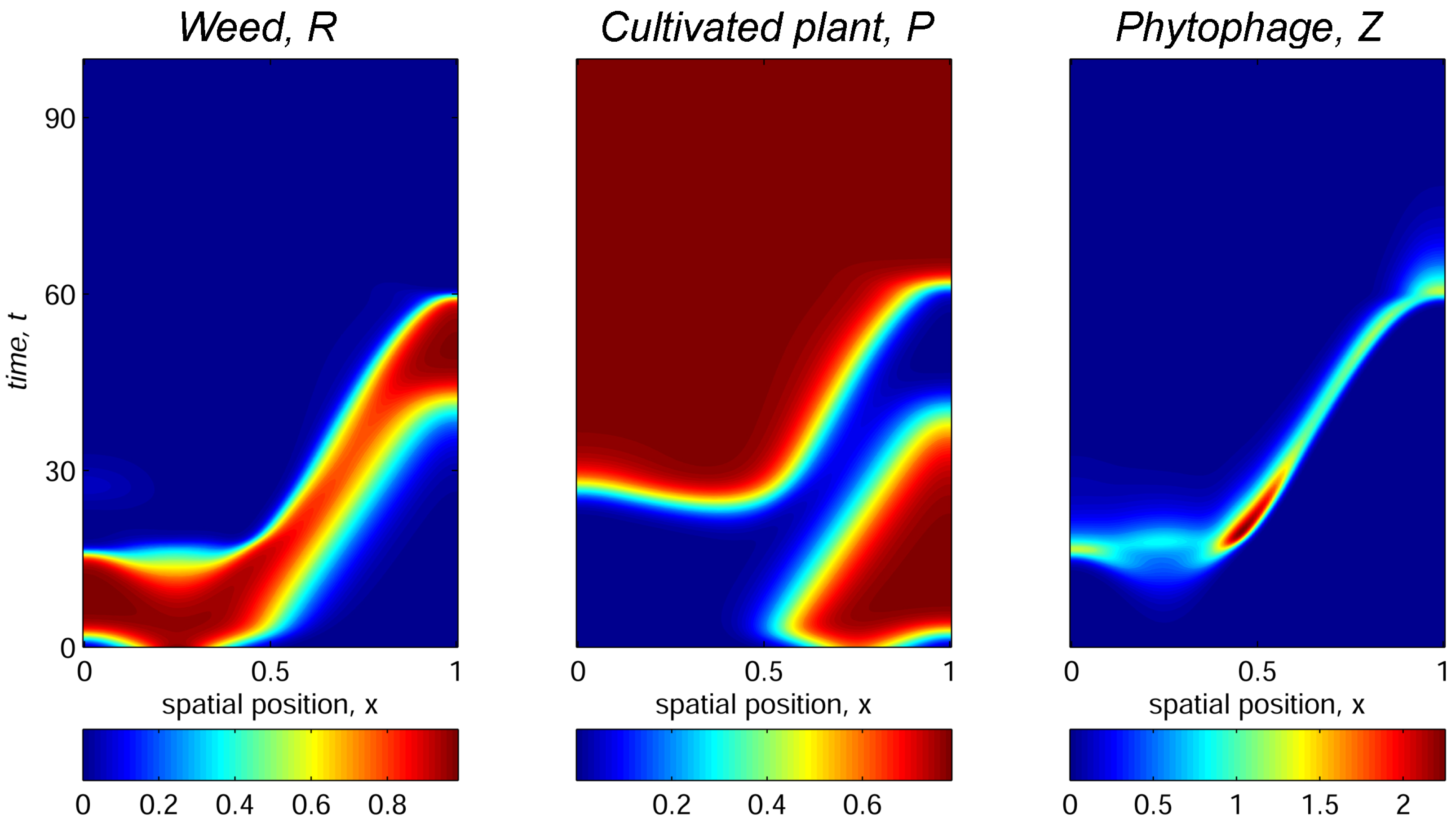
3.2. Case of 1D Spatial Domain

Numerical experiments reveal that, due to accounting for spatial effects, even the 1D version of the model demonstrates dependence of the simulated weed control measures on both parameter values and initial distribution of species densities, manifesting the capability of the model to capture conditions determining successful suppression of the weed foci, explaining the synergistic effect of the combined application of classical and phytocenotic methods.

In this section, we consider a homogeneous habitat entirely suitable for vegetation, i.e., $r_R\left(\mathbf{x}\right)\equiv r_R$, $r_P\left(\mathbf{x}\right)\equiv r_P$, presenting results obtained with System (1)–(4) subject to the Neumann boundary conditions (6) on the edges of the 1D habitat domain $\mathsf{\Omega }=[0,1]$, with Set 2 of the model parameter values presented in Table 1, which differs from Set 1 only by the presence of additional parameters characterizing spatial processes in Model (1)–(4). Note that these values correspond to a nondimentionalized model and have no other biological meaning than illustration of the model capability to qualitatively reflect cases of successful and unsuccessful application of the weed control actions.

First, let us analyze how spatial heterogeneity influences the multistability of homogeneous stationary states corresponding to competitive exclusion of either weed or cultivated plant, which was observed for the spatially homogeneous case of the model. Figure 3 shows the calculation results for the following initial distribution of weed, cultivated plant, phytophage, and trophotaxis stimulus:

$$\begin{array}{c}\hfill \begin{array}{cc}\hfill & {\phi }_R\left(x\right)=R_0(1+cos\left(\pi x\right));\hfill \\ \hfill & {\phi }_P\left(x\right)=P_0(1+cos\left(\pi (1-x)\right));\hfill \\ \hfill & {\phi }_Z\left(x\right)=Z_0(1+cos\left(\pi x\right));\hfill \\ \hfill & {\phi }_S\left(x\right)=0.\hfill \end{array}\end{array}$$

This form of initial distribution depending on total abundances $R_0$ and $P_0$ allows comparison with Figure 2 for $Z_0=0.0006$, which presents the results for the nonspatial model (7). Figure 3 shows basins of attraction to the two spatially homogeneous solutions on the plane $R_0,P_0$ for different values of parameter $\kappa$.

One can see both similarity and differences with the results presented in Figure 2. In particular, Figure 3 shows that, in the case of nonuniform initial distribution, initial prevalence of the cultivated plant does not ensure suppression of the weed. Quite the opposite, at least with small trophotaxis coefficient $\kappa$, successful control of the weed requires prevailing of the weed over the plant phytomass. Figure 3 suggests that increasing ability of phytophagous agent to perform trophotaxis movements strongly impacts its capacity to control the weed, determining the overall success of the biological control strategy. Moreover, higher values of the taxis coefficient in this experiment, e.g., $\kappa >0.05$, ensure total suppression of the weed by the cultivated plant with any combination of initial abundances $R_0$ and $P_0$. Moreover, according to our observations, successful suppression of weeds in the spatial model (1)–(4) can be achieved with much lower initial abundance of the phytophage population than in the point model (7), e.g., with $Z_0=0.00014$.

Next, with the same parameters of Set 2 presented in Table 1, we analyzed the mechanism providing synergistic effect of complex application of classical and phytocenotic methods of weed control, specifying the initial distributions of weed, cultivated plant, and phytophagous biocontrol agent in order to consider separation of weed-infested and cultivated areas, and the concentrated release of phytophagous insects in the zone of maximum weed density. Namely, the initial conditions (5) were specified using a bell-shaped distribution functions normalized over the habitat domain as follows:

$$\begin{array}{c}\hfill \begin{array}{cc}\hfill & {\phi }_R\left(x\right)=R_0·0.{24911}^{-1}·e^{-50{\left(\frac{1}{4}-x\right)}^2};\hfill \\ \hfill & {\phi }_P\left(x\right)=P_0·0.{24911}^{-1}·e^{-50{\left(\frac{3}{4}-x\right)}^2};\hfill \\ \hfill & {\phi }_Z\left(x\right)=Z_0·0.{07927}^{-1}·e^{-500{\left(\frac{1}{k}-x\right)}^2};\hfill \\ \hfill & {\phi }_S\left(x\right)=0,\hfill \end{array}\end{array}$$

(8)

where $R_0$, $P_0$, and $Z_0$ are the initial abundances of weed, plant, and phytophage populations, respectively, and parameter k specifies spatial position of the phytophage releasing. The results in Figure 4, Figure 5 and Figure 6 were obtained with initial distributions (8) computed with $R_0=0.25$, $P_0=0.15$, $Z_0=0.00016$, and $k=4$, which corresponds to preferable release of the insects in the left part of domain $\mathsf{\Omega }$ with maximum initial weed infestation, while the cultivated plant is concentrated in the right part of the habitat. The trophotaxis coefficient is $\kappa =0.17$.

As shown in Figure 4, concentrated release of phytopages in the maximally infested plot is a conductive factor leading to a favorable scenario; after local outbreak, the phytophage population forms SPWs, which move over the whole domain, destroying the weed and facilitating its replacement by the cultivated plant.

Figure 5 shows the result obtained with the hypothetical assumption of the absence of a cultivated plant competing with the weed. As in the previous case, in the beginning, we observe strong growth in the weed population, which now easily occupies the whole domain, providing the feeding resource for local outbreak of the phytophagous insects that form SPWs, which rapidly move through the habitat, wiping out the weed. However, since the result of the SPW action in this scenario is not fixed by cultivated plants, a secondary focus of the weed emerges, giving rise to developing of a new wave of the phytophagous agent, which loops the wave process iteratively. As a result, at each point of the habitat, the weed density periodically grows and then drops to a negligible level, causing local extinction of the phytophage due to the Allee effect affecting its growth, but the ability of the phytophagous insects to perform active feeding migrations prevents global extinction of the biocontrol agent. This particular case of Model (1)–(6) excluded from consideration the cultural plant species that was exhaustively studied in [22].

Simulations considering competing weeds and cultivated plants without introduction of the phytophagous insects produces unsuccessful scenarios corresponding to exclusion of the cultural plant by the weed; see Figure 6.

Numerical experiments with the given parameter values demonstrate the multistability effect consisting of dependence of the model dynamics (and efficacy of the biological method actions) on the initial conditions. Biological interpretation of the simulation results emphasizes the fact that incorrect choice of the release point outside the weed-infested area can cause waste of the agents. With $k=4$ in (8), the initial peak of the phytophage density distribution in Figure 4 coincides with the maximum regarding weed density. According to simulations, moderate shifts in the peak of the phytophage initial distribution within the patch of the weed density also end with weed suppression. However, release of insects at the maximum point of the cultivated plant density $(k=\frac{4}{3})$ causes rapid extinction of the phytophage and exclusion of the cultivated plant by the weed. Decreasing by half the initial amount of the insect population also leads to a negative scenario, and vice versa: increasing it by half speeds up the weed suppression.

The demonstrated dependence of the model dynamics on the initial conditions supports general recommendations formulated by O.V. Kovalev regarding desired conditions for the release of the biocontrol agent species being a specialized phtophage of the target weed capable of forming SPWs [3,11,12,17]. In particular, it was noticed that releasing the phytophage far away from the weed foci or with insufficient released insects leads to phatophage extinction and cannot ensure the phytophage outbreak, which is a necessary phase of SPW formation [15].

Aside from spatially heterogeneous dynamics of the weed–phytophage system (Figure 5) and stationary modes corresponding to exclusion of either cultivated plant or weed (Figure 4 and Figure 6), more complex dynamic spatiotemporal scenarios of all three species’ coexistence are possible. We illustrate this by varying the trophotaxis coefficient $\kappa$ with Set 3 of the model parameter values presented in Table 1 and $k=4$ in the initial distribution of species (8). With these parameters, ignoring the trophotaxis behavior of phytophagous insects, i.e., setting $\kappa =0$, the model approaches spatially homogeneous periodicity in time dynamics, which corresponds to the stable limit cycle of coexistence of all three modeled species in the nonspatial system (7). This scenario is presented in Figure 7.

However, as seen in Figure 8, sufficiently large value of the trophotaxis coefficient, e.g., $\kappa =0.14$, destabilizes the homogeneous limit cycle, and spatially inhomogeneous periodicity in time dynamics emerges. Higher values of the taxis coefficient provide more complex nonperiodicity in time spatiotemporal solutions. Figure 9 shows irregular dynamics obtained with $\kappa =0.7$.

Similar effects of the taxis-induced destabilization of spatially homogeneous periodic regime, causing emergence of spatially heterogeneous dynamics, undergoing further transformations to quasi-periodic and chaotic regimes with increase in the prey taxis coefficient, have been observed previously in simpler predator–prey models with indirect prey taxis of the predator, which did not take into account the population competing with the prey [10,22].

Regarding interpretation of the obtained results in terms of the biological control problems, summarizing outcomes of the current section, we can conclude that, under plausible assumptions, Model (1)–(6) is capable of reproducing successful (Figure 4), unsuccessful (Figure 6), and partial control of the weed with either regular (as in Figure 7 and Figure 8) or irregular (as in Figure 9) outbreaks of the weed, followed by relatively satisfactory periods of weed suppression.

3.3. Case of 2D Spatial Domain

Presenting an example of simulations with heterogeneous 2D rectangular spatial domain $\mathsf{\Omega }=[0,L_x]\times [0,L_y]$, we use parameter values borrowed from the model of trophic system consisting of the common ragweed Ambrosia artemisiifolia L. and the ragweed leaf beetle Zygogramma suturalis F. (Coleoptera, Chrysomelidae) [15], presented in Set 4 of Table 1 along with the supplementary parameters characterizing the cultivated plant.

Note that, in the absence of phytophage population and with homogeneous distribution of weed and cultivated plant, the dynamics of the System (1)–(4) in a homogeneous habitat with the Neumann boundary condition (6) obey the classical nonspatial Lotka–Volterra model of two species competition [26,27]:

$$\begin{array}{c}\hfill \begin{array}{cc}\hfill & \frac{dR}{dt}=R(r_R-c_{R}R-c_{RP}P);\hfill \\ \hfill & \frac{dP}{dt}=P(r_P-c_{P}P-c_{PR}R).\hfill \end{array}\end{array}$$

(9)

With the chosen parameters, depending on the initial condition, System (9) predicts competitive exclusion of one or another species, approaching either equilibrium $\left(K_R,0\right)$ or equilibrium $\left(0,K_P\right)$, where $K_R=r_R/c_R=1.17$ $\mathrm{kg}·{\mathrm{m}}^{-2}$ and $K_P=r_P/c_P\approx 0.75$ $\mathrm{kg}·{\mathrm{m}}^{-2}$ are the “carrying capacities” of the weed and cultivated plant, respectively (see Figure 10).

Accounting for spatial effects in 2D, habitat heterogeneity, and inclusion of the phytophage population in the Model (1)–(4) modifies the dynamics of the system, making it more realistic. Figure 11 presents the result of a simulation obtained with a hypothetical heterogeneous habitat $\mathsf{\Omega }=4000\mathrm{m}\times 3000\mathrm{m}$, which includes being unsuitable for vegetation plots, as shown in Figure 11.

The initial conditions of the simulation correspond to homogeneous distribution of high density of the weeds, locally superseded by the cultivated plant (the patch of approximately 3–4 ha in the center of domain $\mathsf{\Omega }$). Additionally, the simulation scenario includes a concentrated local release of 1500 individuals of phytophagous insects in the right part of the domain $\mathsf{\Omega }$. These conditions of the release maximize the efficacy of introduction of the weed biocontrol agents [3,15,17].

According to Figure 11, development of the cultural plant suppresses the weed patch in the center of the domain during the initial phase of the weed control action; however, further expansion of the cultivated plant slows down so that its practical effect becomes almost negligible. Simultaneously, local outbreak of the introduced phytophagous insects forms SPWs with an extremely high density of insects in front, which radically reduces the weed density, expanding over the whole domain and exempting the territory for the cultivated plant competing with the weeds, which fixes the result of the biological method, blocking emergence of secondary foci of the weeds.

4. Discussion and Conclusions

Despite the long (almost two hundred years) experience of classical biocontrol release for weeds, a systemic approach is still lacking to determine the factors of efficacy of biological control actions and to find the most efficient agents. Some authors even describe success in biological control in terms of a lottery model [28]. In practice, a maximal effect may be achieved unexpectedly by using a single introduced phytophagous species [1,6,28], which McEvoy and Coombs [29] called the “silver bullet”. Selection among the potentially effective biocontrol agents and choice regarding the phytophagous insects strictly specific to the targeted adventive weed are traditionally based on analysis of the peculiarities of the species biology [30,31,32,33]. Having analyzed the biocontrol release history records [1,34] and considering his own experience regarding the introduction of the North American ragweed leaf beetle Zygogramma suturalis F. in the Old World, O.V. Kovalev [11,12] revealed that evaluation of the efficacy of a particular weed biocontrol agent should not be based solely on the species biology within its primary range. He suggested that the efficacy of a biological method of weed suppression is determined not so much by the biological characteristics of the released phytophage but by a more complex process that includes conditions ensuring formation of SPW—a systemic phenomenon that can be observed only in the secondary range of the invaded/introduced species, where its growth is not limited by specific enemies and competitors [3,11,13,35,36]. Availability of extended plots with high phytomass of target weeds is an essential condition for SPW emergence, which is also not attainable within the native habitats of species. Another important effect in the systemic process of weed suppression concerns the action of cultural plants competing with weeds, which restores the natural succession in the treated territories after wiping out the weeds behind the expanding SPW of the biocontrol agent [17]. All these circumstances define clear requirements for a mathematical model capable of describing the system dynamics. In particular, the necessity of considering the dispersing population of specialized phytophagous insects introduced into their secondary range infested by the target weed justifies the use of a spatial predator–prey (consumer–resource) model with additional inclusion of the cultural plant competing with the weed (prey) population. The Holling type II trophic function of the phytophagous population with numerical response subject to the Allee effect in Equations (1) and (3) enables a plausible description of the weed consumption, taking into account the possibility of deterministic extinction of the biocontrol agent failing to be established after its unsuccessful introduction. Inclusion of the indirect prey taxis of predators into the Model (1)–(6) is crucial for reproducing spatially heterogeneous dynamics induced solely by the spatial behavior of the predator capable of performing directed movements upward the prey density gradient [37]. The role of prey taxis behavior and of the spatiotemporal wave dynamics in obtaining durable and stable control of the predator over its prey population have been demonstrated earlier in [10].

Even a spatially independent (point) model (7) that corresponds to a homogeneous case of System (1)–(4) reveals an important peculiarity of the modeled community. Analyzing basins of attractions in Figure 2 computed for equilibria $R=1$, $P=0$, $Z=0$ and $R=0$, $P=0.8$, $Z=0$, which correspond, respectively, to the failure and success of the biocontrol program, we can conclude that high initial phytomass of the weed is a crucial prerequisite for efficient release of the biological agent.

Confronting Figure 2 and Figure 3 leads us to another interesting observation. With the given set of parameter values, which, in the absence of a phytophage, corresponds to bistability in the homogeneous model (7), initial domination of the cultivated plant ensures suppression of the weed with any initial abundance of the biocontrol agent population. This is indicated by the fact that the blue triangle in the upper-left part of the $R_0$–$P_0$ plane in Figure 2 is not affected by the $Z_0$ value. However, in a spatial model (1)–(4) (which is undoubtedly more realistic than a point model), in the absence of a phytophage, weeds, which are supposed to differ from the cultivated plant by a larger growth rate, win the competition with any initial density. Figure 3 shows that initial dominance does not provide any advantage to the slower-growing cultivated plant. Moreover, in the presence of phytophages in a sufficient quantity, suppression of weeds by cultivated plants requires initial domination of the weed population. Under such conditions, a spatial model (1)–(4) demonstrates the possibility of biological control even with a diffusively dispersing agent. Adding the ability of performing trophotaxis movements amplifies the phytophage efficacy significantly, providing achievement of success with much lower initial quantity of released insects than is required in a point model (7).

Experiments with a customizable initial distribution of species (8) emphasize the importance of releasing the biocontrol agents within an extended area with high weed density. According to simulation results, violation of this requirement can lead to the extinction of the phytophage population lacking the source of energy for establishing and growth. Thus, the Model (1)–(6) supports recommendations for releasing of the biocontrol agent within a large and dense weed foci with high phytomass in order to ensure the initial outbreak of the phytophage population at the initial phase of the SPW formation [17]. Note that, although locally this outbreak follows the classical pattern of the “bottom-up” regulation of the trophic system, the expanding SPW of the biocontrol agent provides the conditions for systemic “top-down” control, ensuring suppression of the extended dense weed foci [3,13,36]. Thus, both kinds of control, “bottom-up” and “top-down”, can be observed in the system due to the emergent SPW of the phytophage [38]. The expanding SPW is in fact a spatially continuing outbreak of the phytophage population, which would otherwise, in accordance with the typical pattern of population outbreak, collapse in numbers after the explosion phase due to local starvation [39,40].

A simulation performed with a 2D habitat (Figure 11) presents an example of using the model in an earlier applied study [15], describing the action of the SPW of the ragweed leaf beetle that suppresses common ragweed and emphasizing the synergistic effect of combined application of the phytophagous insect and cultivated plant, which was added into the simulation scenario.

In sum, we can conclude that, despite its comparatively simple structure, the spatial model (1)–(6) is capable of reproducing quite complex dynamics of the considered trophic system, adequately describing the systemic process of weed suppression that includes the initial arrangement of biocontrol action, release of the phytophagous agent, local outbreak of phytophage population, formation and movement of SPW wiping the area, and replacement of remaining weeds with cultivated plants, consolidating the final result. The model helps to reveal a number of key aspects relating to factors that determine success in biological control. Importantly, the modeling outcomes coincide with practical recommendations for achieving maximum efficacy regarding biocontrol application.

References

1. McFadyen, R.E.C. Successes in biological control of weeds. In Proceedings of the X International Symposium on Biological Control of Weeds, Bozeman, MT, USA, 4–14 July 1999; Spencer, N.R., Ed.; Montana State University: Bozeman, MT, USA, 2000; pp. 3–14. Available online: https://www.invasive.org/publications/xsymposium/proceed/01apg03.pdf (accessed on 29 November 2023).
2. Cuda, J.P.; Charudattan, R.; Grodowitz, M.J.; Newman, R.M.; Shearer, J.F.; Tamayo, M.L.; Vilegas, B. Recent advances in biological control of submersed aquatic weeds. J. Aquat. Plant Manag. 2008, 46, 15–32. [Google Scholar]
3. Kovalev, O.V.; Tyutyunov, Y.V. The role of solitary population waves in efficient suppression of adventive weeds by introduced phytophagous insects. Entmol. Rev. 2014, 94, 310–319. [Google Scholar] [CrossRef]
4. Mason, P. (Ed.) Biological Control: Global Impacts, Challenges and Future Directions of Pest Management; CSIRO Publishing: Canberra, Australia, 2021; 626p. [Google Scholar]
5. López-Núñez, F.A.; Marchante, E.; Heleno, R.; Duarte, L.N.; Palhas, J.; Impson, F.; Freitas, H.; Marchante, H. Establishment, spread and early impacts of the first biocontrol agent against an invasive plant in continental Europe. J. Environ. Manag. 2021, 290, 112545. [Google Scholar] [CrossRef] [PubMed]
6. Shaw, R.H.; Ellison, C.A.; Marchante, H.; Pratt, C.F.; Schaffner, U.; Sforza, R.F.H.; Deltoro, V. Weed biological control in the European Union: From serendipity to strategy. BioControl 2018, 63, 333–347. [Google Scholar] [CrossRef]
7. Luck, R.F. Evaluation of natural enemies for biological control: A behavioral approach. Trends Ecol. Evol. 1990, 5, 196–199. [Google Scholar] [CrossRef] [PubMed]
8. Arditi, R.; Berryman, A.A. The biological control paradox. Trends Ecol. Evol. 1991, 6, 32. [Google Scholar] [CrossRef] [PubMed]
9. Berryman, A. The theoretical foundations of biological control. In Theoretical Approaches to Biological Control; Hawkins, B., Cornell, H.V., Eds.; Cambridge University Press: Cambridge, UK, 1999; pp. 3–21. [Google Scholar]
10. Sapoukhina, N.; Tyutyunov, Y.; Arditi, R. The role of prey-taxis in biological control: A spatial theoretical model. Am. Nat. 2003, 162, 61–76. [Google Scholar] [CrossRef]
11. Kovalev, O.V. The solitary population wave, a physical phenomenon accompanying the introduction of a chrysomelid. In New Developments in the Biology of Chrysomelidae; Jolivet, P., Ed.; SPB Academic Publishing BV: The Hague, The Netherlands, 2004; pp. 591–601. [Google Scholar] [CrossRef]
12. Kovalev, O.V. Spread of adventive plants of Ambrosieae tribe in Eurasia and methods of bilogical control of Ambrosia L. (Asteraceae). In Theoretical Principles of Biological Control of the Common Ragweed, Proceedings of the Zoological Institute; Kovalev, O.V., Belokobylsky, S.A., Eds.; “Nauka” Publishing House, Leningrad Branch: Leningrad, Russia, 1989; Volume 189, pp. 7–23. (In Russian) [Google Scholar]
13. Kovalev, O.V.; Tyutyunov, Y.V.; Iljina, L.P.; Berdnikov, S.V. On the efficiency of introduction of american insects feeding on the common ragweed (Ambrosia artemisiifolia L.) in the South of Russia. Entomol. Rev. 2013, 92, 251–264. [Google Scholar] [CrossRef]
14. Vechernin, V.V.; Kovalev, O.V. New mathematical model of a solitary wave for describing a population wave. Biophysics 1988, 33, 701–707. [Google Scholar]
15. Tyutyunov, Y.V.; Kovalev, O.V.; Titova, L.I. Spatial demogenetic model for studying phenomena observed upon introduction of the ragweed leaf beetle in the south of Russia. Math. Model. Nat. Phenom. 2013, 8, 80–95. [Google Scholar] [CrossRef]
16. Tyutyunov, Y.V. Spatial demo-genetic predator–prey model for studying natural selection of traits enhancing consumer motility. Mathematics 2023, 11, 3378. [Google Scholar] [CrossRef]
17. Kovalev, O.V.; Tyutyunov, Y.V.; Arkhipova, O.E.; Kachalina, N.A.; Iljina, L.P.; Titova, L.I. On assessment of the large-scale effect of introduction of the ragweed leaf beetle Zygogramma suturalis F. (Coleoptera, Chrysomelidae) Phytocenoses South Russia. Entomol. Rev. 2015, 95, 1–14. [Google Scholar] [CrossRef]
18. Allee, W. Animal Aggregations: A Study in General Sociology; Chicago University Press: Chicago, IL, USA, 1931; 431p. [Google Scholar]
19. Dennis, B. Allee effects: Population growth, critical density, and the chance of extinction. Nat Resour Model. 1989, 3, 481–538. [Google Scholar] [CrossRef]
20. Bazykin, A.D. Nonlinear Dynamics of Interacting Populations; World Scientific Publishing: Singapore, 1998; 193p. [Google Scholar]
21. Courchamp, F.; Berec, J.; Gascoigne, J. Allee Effects in Ecology and Conservation; Oxford University Press: Oxford, NY, USA, 2008; 256p. [Google Scholar]
22. Tyutyunov, Y.; Sen, D.; Titova, L.I.; Banerjee, M. Predator overcomes the Allee effect due to indirect prey-taxis. Ecol. Complex. 2019, 39, 100772. [Google Scholar] [CrossRef]
23. Hairer, E.; Nørsett, S.; Wanner, G. Solving Ordinary Differential Equations I. Nonstiff Problems; Springer: Berlin/Heidelberg, Germany, 2009; 528p. [Google Scholar]
24. Budyansky, A.V.; Frischmuth, K.; Tsybulin, V.G. Cosymmetry approach and mathematical modeling of species coexistence in a heterogeneous habitat. Discrete Contin. Dyn. Syst.-Ser. B 2019, 24, 547–561. [Google Scholar] [CrossRef]
25. Govorukhin, V.N.; Zagrebneva, A.D. Population waves and their bifurcations in a model “active predator–passive prey”. Comput. Res. Model. 2020, 12, 831–843. (In Russian) [Google Scholar] [CrossRef]
26. Gause, G.F.; Witt, A.A. Behavior of mixed populations and the problem of natural selection. Am. Nat. 1935, 69, 596–609. [Google Scholar] [CrossRef]
27. Mallet, J. The struggle for existence: How the notion of carrying capacity, K, obscures the links between demography, Darwinian evolution, and speciation. Evol. Ecol. Res. 2012, 14, 627–665. [Google Scholar]
28. Myers, J.H. How many insect species are necessary for successful biocontrol of weeds? In Proceedings of the VI International Symposium on Biological Control of Weeds, Vancouver, BC, Canada, 19–25 August 1984; Delfosse, E.S., Ed.; Agriculture: Vancouver, BC, Canada, 1985; pp. 77–82. [Google Scholar]
29. McEvoy, P.B.; Coombs, E.M. Biological control of plant invaders: Regional patterns, field experiments, and structured population models. Ecol. Appl. 1999, 9, 387–401. [Google Scholar] [CrossRef]
30. Briese, D.T. Classical biological control. In Australian Weed Management Systems; Sindel, B.M., Ed.; R.G. & F.J. Richardson: Melbourne, Australia, 2000; pp. 161–192. [Google Scholar]
31. Van Klinken, R.D.; Raghu, S. A scientific approach to agent selection. Aust. J. Entomol. 2006, 45, 253–258. [Google Scholar] [CrossRef]
32. Müller-Schärer, H.; Schäffner, U. Classical biological control: Exploiting enemy escape to manage plant invasions. Biol. Invasions 2006, 10, 859–874. [Google Scholar] [CrossRef]
33. Schwarzländer, M.; Hinz, H.L.; Winston, R.L.; Day, M.D. Biological control of weeds: An analysis of introductions, rates of establishment and estimates of success, worldwide. BioControl 2018, 63, 319–331. [Google Scholar] [CrossRef]
34. Julien, M.N.; Griffiths, M.W. Biological Control of Weeds: A World Catalogue of Agents and Their Target Weeds, 4th ed.; CABI Publishing: Wallingford, UK, 1998; 223p. [Google Scholar]
35. Kovalev, O.V.; Medvedev, L.N. Theoretical basis of introduction of ragweed leaf beetles of the genus Zygogramma Chevr. (Coleoptera: Chrysomelidae) in the USSR for biological control of ragweed. Entomol. Obozr. 1983, 62, 17–32. (In Russian) [Google Scholar]
36. Kovalev, O.V. New factor of efficiency of phytophages: A solitary population wave and succession process. In Proceedings of the VII International Symposium on Biological Control of Weeds, Rome, Italy, 6–11 March 1988; Delfosse, E.S., Ed.; Ministero dell’Agricoltura e delle Foreste: Rome, Italy; CSIRO: Melbourne, Australia, 1990; pp. 51–53. [Google Scholar]
37. Arditi, R.; Tyutyunov, Y.; Morgulis, A.; Govorukhin, V.; Senina, I. Directed movement of predators and the emergence of density-dependence in predator-prey models. Theor. Popul. Biol. 2001, 59, 207–221. [Google Scholar] [CrossRef]
38. Ginzburg, L.R.; D’Andrea, R. Trophic Levels. In Encyclopedia of Biodiversity, 3rd ed.; Scheiner, S.M., Ed.; Academic Press: Oxford, UK, 2024; Volume 5, pp. 252–258. [Google Scholar] [CrossRef]
39. White, T.C.R. The Inadequate Environment: Nitrogen and the Abundance of Animals; Springer: Berlin, Germany, 1993; 425p. [Google Scholar]
40. White, T.C.R. Why Does the World Stay Green?: Nutrition and Survival of Plant-Eaters; CSIRO Publishing: Collingwood, Australia, 2005; 120p. [Google Scholar]
Figure 1. Dynamics in homogeneous case, R 0 = 0.9 , P 0 = 0.1 : (a) Z 0 = 0.0004 , (b) Z 0 = 0.00050729 , (c) Z 0 = 0.001 .
Mathematics 12 00160 g001
Figure 2. Basins of attraction for equilibria R = 1 , P = 0 , Z = 0 (red) and R = 0 , P = 0.8 , Z = 0 (blue) computed for three different initial values Z 0 .
Mathematics 12 00160 g002
Figure 3. Basins of attraction for stationary states R = 1 , P = Z = 0 (red) and R = Z = 0 , P = 0.8 (blue) computed for Z 0 = 0.0006 without taxis (left panel) and with taxis: κ = 0.002 (central panel); κ = 0.005 (right panel).
Mathematics 12 00160 g003
Figure 4. Spatiotemporal dynamics of the model, illustrating successful suppression of weed due to synergistic effect of the combined application of phytophagous insects and cultivated plant competing with the weed.
Mathematics 12 00160 g004
Figure 5. Numerical simulation corresponding to scenario in which result of the phytophage SPW passage is not fixed by the cultivated plant competing with the weed.
Mathematics 12 00160 g005
Figure 6. Numerical result obtained for the scenario, which envisages unsuccessful attempt to suppress the weed by cultivated plant without the use of phytophage.
Mathematics 12 00160 g006
Figure 7. Stabilization of uniformity in space and periodicity in time dynamics; κ = 0 .
Mathematics 12 00160 g007
Figure 8. Stabilization of nonuniformity in space and periodicity in time dynamics; κ = 0.14 .
Mathematics 12 00160 g008
Figure 9. Stabilization of nonuniformity in space and nonperiodicity in time dynamics; κ = 0.7 .
Mathematics 12 00160 g009
Figure 10. Phase portrait of the point model (9). Locally stable equilibria are represented by solid dots; unstable equlibria are represented by hollow dots. The dashed line is the separatrix, dividing the positive quadrant of the phase plane into basins of attraction of axial equlibria corresponding to exclusion of either weed or cultivated plant.
Mathematics 12 00160 g010
Figure 11. Snapshots of spatial distribution of population densities at the indicated moments of time, computed with model (1)–(6) for hypothetical heterogeneous spatial domain Ω = 4000 m × 3000 m .
Mathematics 12 00160 g011