Article

Three-Dimensional Lidar Localization and Mapping with Loop-Closure Detection Based on Dense Depth Information

1
School of Computer Science, University of Electronic Science and Technology of China, Zhongshan Institute, Zhongshan 528402, China
2
School of Automation Engineering, University of Electronic Science and Technology of China, Chendu 611731, China
3
School of Automation, Guangdong University of Technology, Guangzhou 510006, China
*
Author to whom correspondence should be addressed.
These authors contributed equally to this work.
Mathematics 2023, 11(9), 2211; https://doi.org/10.3390/math11092211
Submission received: 19 March 2023 / Revised: 22 April 2023 / Accepted: 1 May 2023 / Published: 8 May 2023
(This article belongs to the Section Engineering Mathematics)

Abstract

:
This paper presents a novel lidar SLAM system for localizing a mobile robot to build a map of the environment. To identify the unknown transform matrix, we design a new scan-matching approach, in which a point cloud segmentation algorithm is additionally integrated. Different from the traditional normal distribution transform algorithm for point cloud registration, our newly proposed one additionally incorporates a ground point remover and a point cloud segmentation method. By employing the point cloud segmentation algorithm to divide the point cloud space into different cells, the newly proposed algorithm can guarantee the continuity and convergence of the cost function. To tackle the recognition difficulties that the camera-based loop-closure detection heavily depends on the environment’s appearance, a depth-completion algorithm is introduced to fuse sensor data to ensure the robustness of the algorithm. Moreover, the bags of binary words (DBoW) are adopted to improve the image-matching quality. Finally, experimental results are presented to illustrate the effectiveness of the proposed system.
MSC:
93-08; 93-10

1. Introduction

In the last ten years, simultaneous localization and mapping (SLAM) has drawn increasing attention from both scientific and industrial communities, due to its various applications such as environmental reconstruction, exploration, autonomous driving vehicles, etc. Generally, the SLAM problem can be described as a state estimation problem as seen from [1,2,3,4,5,6]. In [1], a random sampling approach was developed to deal with the state of estimation for systems under measurement noise. In [2], Rao–Blackwellized particle filters (RBPFs) were designed to improve the accuracy of pose estimation by utilizing the structure of a dynamic Bayesian network(DBN). Furthermore, Grisetti et al. developed an RBPF based system [3] to tackle the particle depletion problem by designing a new adaptive technique to reduce the number of particles and a good performance was guaranteed. In [4], a laser-ranger-finder-based algorithm was proposed to achieve simultaneous localization and mapping by designing a new distributed particle mapping, which successfully removed the assumption that predetermined landmarks should be employed in the environment. To make up for the noise problem caused by the inherent assumptions of EKF SLAM, a hybrid filtering SLAM method was proposed by integrating the neural network and the EKF algorithm [5]. An observability-constrained unscented Kalman filter SLAM method with sampling strategy for the UK was presented to improve the accuracy and consistency of state estimates [6]. Moreover, by combining an extended Kalman filter and an iterative SfM algorithm, a new control scheme was proposed and exhibited better robustness to outliers in [7]. However, these Kalman filtering based methods only considered the impact of the state of previous moments on the state of the current moment, which lost a lot of information from past moments. In the proposed approach, more information from past moments are considered and cumulative estimation errors can be further corrected by a closed-loop detection, which is integrated into our control scheme. To alleviate the computation burden, Kohlbrecher proposed a scheme based on Gauss–Newton to deal with the scan-matching problem [8]. Furthermore, a flexible and scalable 3D attitude estimation system was developed to cope with robots learning maps in unknown environments, which successfully incorporated the IMU data into the state estimation. However, the early works mentioned above did not take into account the effect of cumulative errors on the accuracy of mapping buildings. In practice, cumulative errors in large-scale scenarios are essentially important for a SLAM system to improve the accuracy of mapping buildings.
To tackle this challenging problem, up to now, some interesting results have been reported in [9,10]. In [9], an efficient sparse pose adjustment method was proposed to reduce the cumulative error by transforming a large optimizing pose graph problem into solving a linear subproblem. In [10], Hess et al. developed a new SLAM system by proposing a branch-and-bound approach. To realize a 3D map construction, much effort has been spent in [11,12,13,14]. In [11], a point cloud registration algorithm was proposed, which successfully solved the relative pose transformation problem through the correspondence between two pairs of point clouds. It was further extended to 3D mapping tasks by Magnusson [12]. In [13], Zhang et al. successfully tackled the feature-matching problem by utilizing the Levenberg–Marquardt method to optimize the loss function. Subsequently, by designing a new ground extraction algorithm and refactoring the code, Shan [14] proposed a LEGO-LOAM solution and an excellent performance was guaranteed, which was successfully applied in the six degree-of-freedom pose estimation of ground vehicles. In particular, a graph-based SLAM approach was designed using directional endpoint features for the efficient initialization and updating in [15]. To address the unreliability of GPS-based localization, Jung et al. further proposed a novel hierarchical-graph-based SLAM method to ensure the system stability by using NDT and G-ICP matching methods [16]. Moreover, a tightly coupled multisensor fusion framework was constructed to achieve a robust and accurate state estimation by utilizing filter-based odometry and factor graph optimization in [17].
Inspired by the prior works mentioned above, this paper presents a 3D lidar localization and mapping solution based on dense depth information. One of the main difficulties hindering the development of this solution is how to use the characteristics of different sensors to improve the perception ability of robots. To remove this obstacle, a novel loop closure detection is proposed in this paper. Based on depth completion, we convert the sparse depth information obtained from the lidar data into a dense depth image and use mature visual methods to achieve loop-closure detection. The main contributions of this paper are as follows.
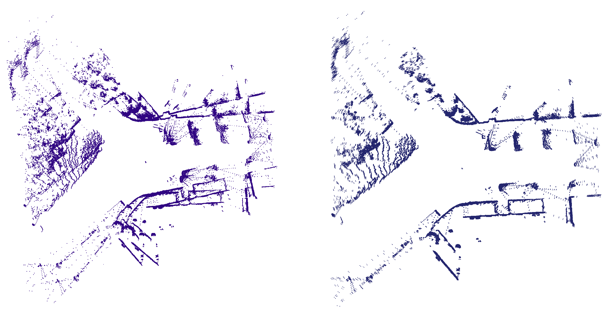
  • In comparison with the previous scan-matching algorithm in [12], our newly proposed one additionally contains a ground-point removal and an effective point cloud data segmentation algorithm. To overcome the slow convergence speed arising from the inaccurate environment model, the point cloud registration problem has been successfully transformed into an optimization problem. Subsequently, a point cloud segmentation algorithm is newly designed to divide the point cloud space into different cells, which exhibits an excellent performance.
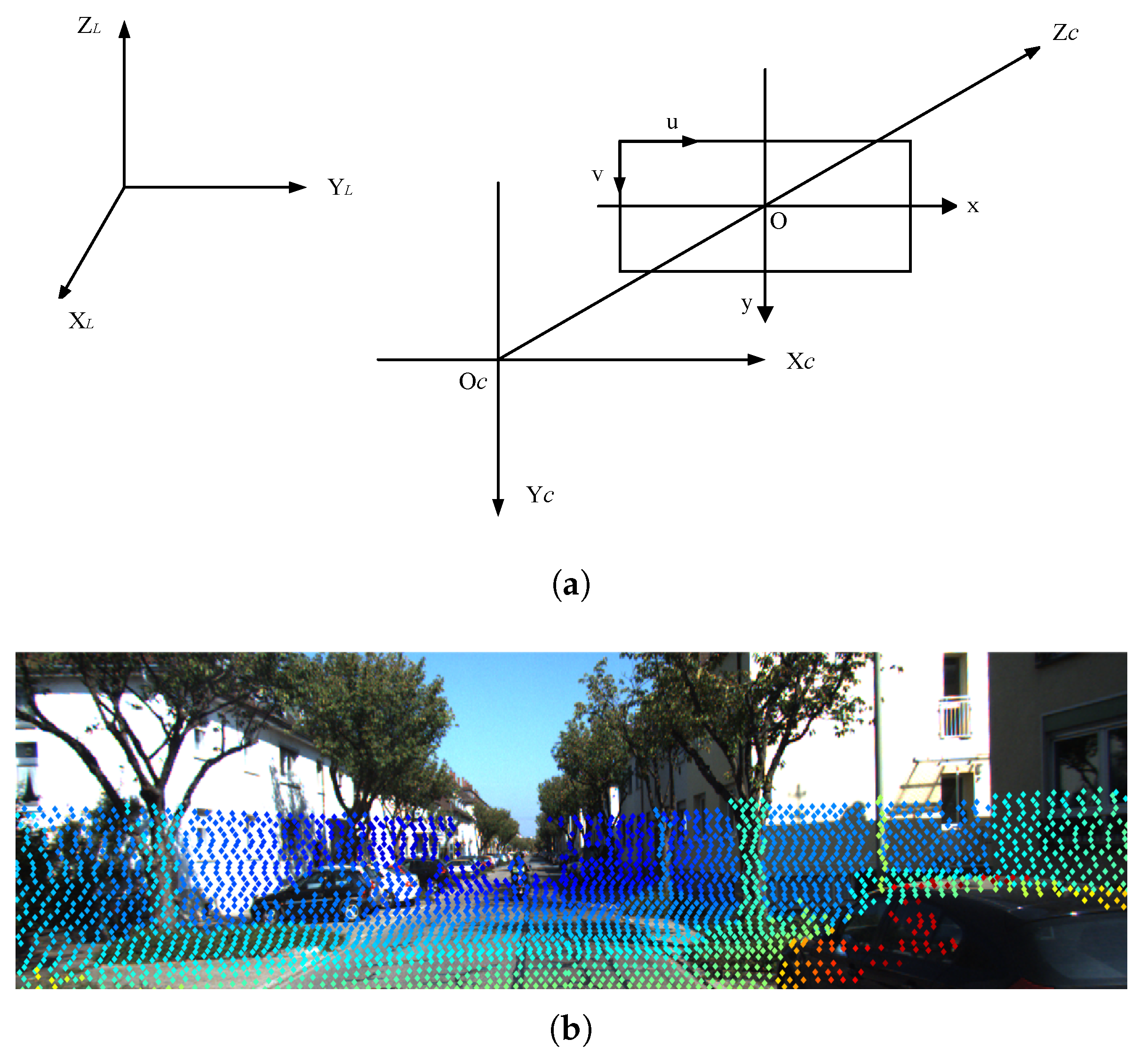
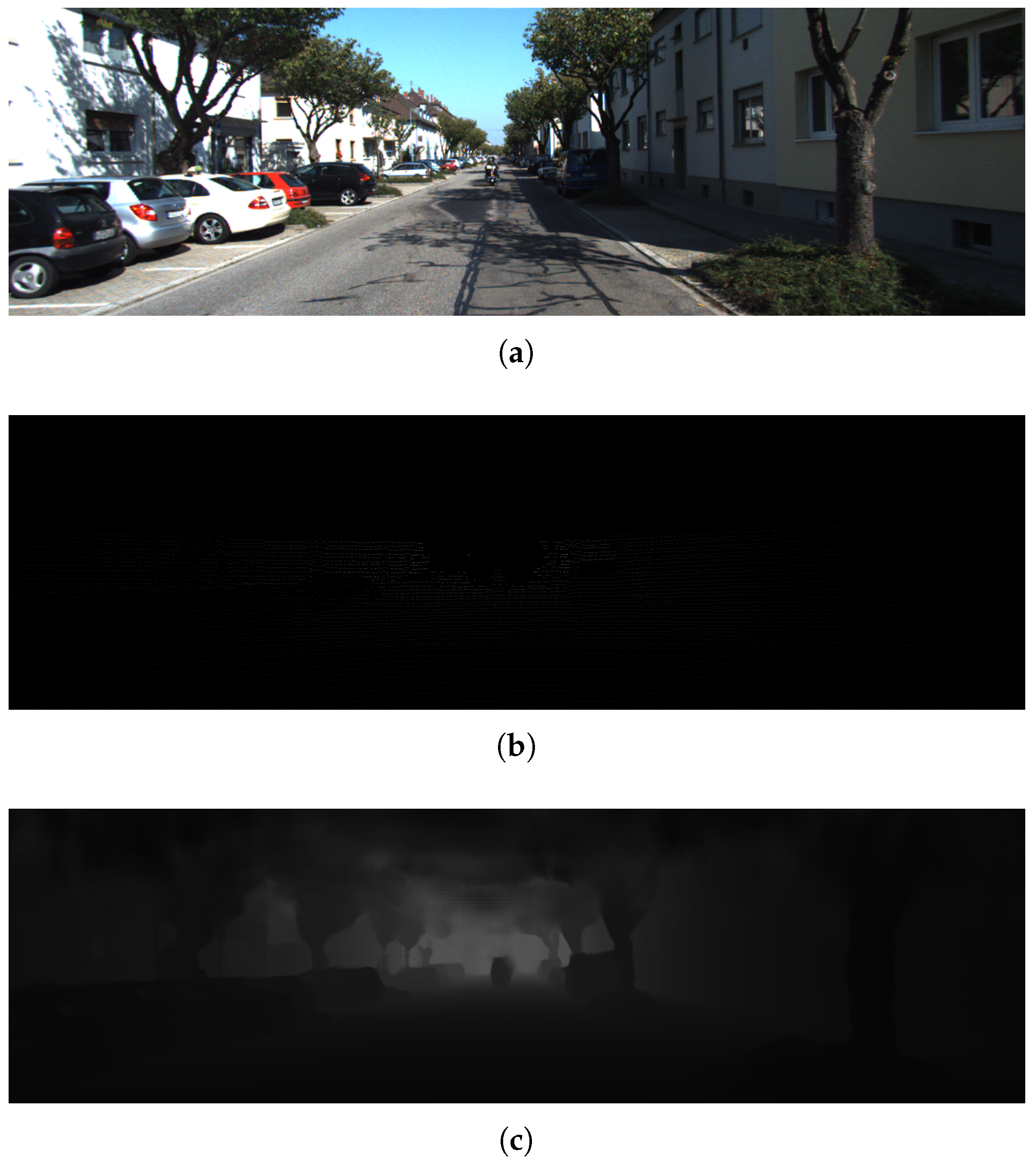
  • By fusing lidar data with camera data, our newly proposed loop-closure detection scheme successfully avoids the common problem found in [8] that loop-closure detection is prone to fail in structured scenes. In comparison with common vision schemes, our proposed scheme can effectively reduce the influence of the illumination on the loop-closure detection with the aid of a depth-completion algorithm, and thus our scheme is more robust in various scenarios.

2. Related Work

For the SLAM problem, the uncertainty of localization and map building can be handled by the state estimation theory, and the uncertainty of the state can be estimated by nonlinear optimization algorithms. In lidar SLAM, a mobile robot obtains the point cloud data of the environment through lidar and, using a point cloud registration algorithm, the method estimates the relative pose and realizes the motion estimation of the mobile robot.As the scale of the map increases, the global consistency of the map will continue to decline, resulting in dislocation and ghosting. To solve this problem, SLAM systems are usually equipped with a loop-closure detection module, which can correct the global pose by detecting whether the mobile robot is located at a previously visited location.
The initial lidar odometry is primarily accomplished by the ICP algorithm. However, the ICP algorithm is limited by its assumptions. Since the point cloud data are usually sparse, it is difficult to a one-to-one correspondence between points. To address its shortcoming, many important works have been proposed. In [18], Aleksandr proposed the G-ICP algorithm to extend the probability model of the locally planar structure to the global one. In [19], the NICP algorithm not only restricted the distance between points but also added constraints on the normal vector and the curvature of the surface where the point cloud was located. In [12], the NDT algorithm was proposed, in which the distribution characteristics of point clouds were utilized to achieve registration. Compared with the ICP algorithm, it did not require the assumption of a corresponding relationship between point clouds and considerably improved the calculation speed and accuracy. To improve the performance of the NDT algorithm, much effort has been spent in [20,21,22]. These methods improved the accuracy of the NDT algorithm by improving the cost function and clustering point clouds. For the dense 3D point cloud, some scholars have proposed to use the characteristic points of the point cloud to realize the lidar odometry, and LOAM is the most representative one.
In traditional lidar-based loop-closure detection, some methods based on point cloud matching [23] do not need to process point cloud data and directly use the registration algorithm for matching. However, they require a lot of calculations in large-scale scenes and require high initial conditions. Methods based on point cloud feature description such as scan context [24], intensity scan context [25] and IRIS [26] can achieve point cloud closed loop detection in large-scale scenes. However, these methods are likely to fail if the scanning angle of the lidar changes. In visual SLAM, a camera can obtain rich environmental texture information, and many mature methods are used to detect and match it, among which the word-bag model is the most widely used. By using DBoW [27] to transform the extracted visual features into bag vectors, another description of the image is obtained, which is used to match the similarity between images. However, the camera-based approach is sensitive to the light and viewpoint and is not particularly stable.

3. Proposed Method

To improve the accuracy of the lidar odometry, gain a more accurate initial pose estimation and use a more robust loop-closure detection algorithm to improve the consistency of the map, a complete 3D lidar SLAM system is proposed, which includes a lidar odometry based on a point cloud segmentation and loop-closure detection on dense depth information.

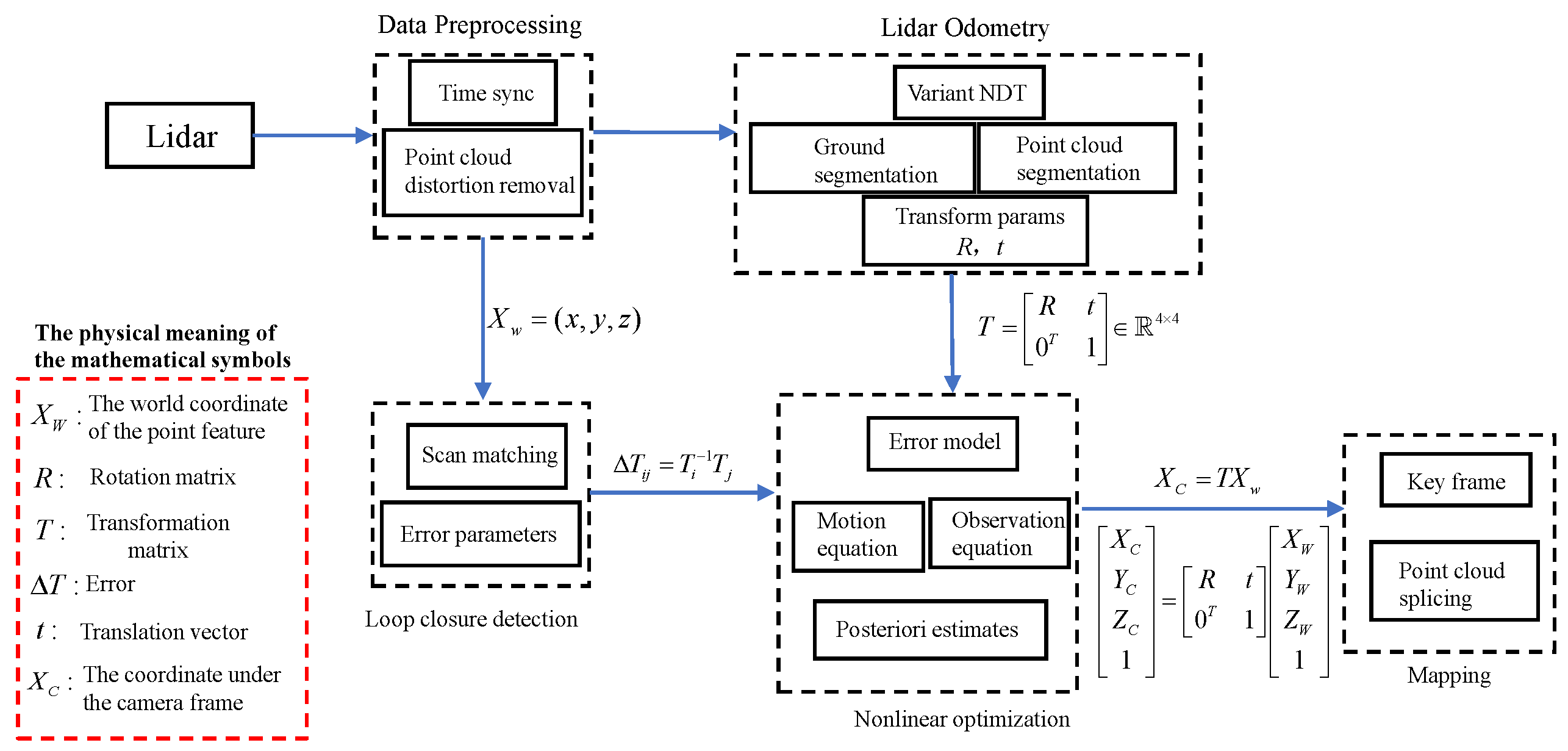
3.1. System Overview

The SLAM system proposed in this paper consists of five modules including data preprocessing, lidar odometry, loop-closure detection, back-end and mapping. The main work of the data pretreatment module is time synchronization and the basic cutting processing of various sensor data. The lidar odometry is realized by using the NDT variant algorithm, by removing ground points from point cloud data and segmenting the point cloud according to whether they belong to the same object. Then, a Gaussian distribution is constructed in each subspace for the initial pose estimation. In the loop detection part, the camera data and lidar data are combined. The global retrieval of local maps is realized by using the depth-completion algorithm and the visual-bag-of-words model. After the corrected pose is obtained, it is sent to the back-end optimization module for calculation. The back-end optimization module uses the G2O [28] library to build the model of nodes and edges and optimize the global pose. The map-building module uses the optimized pose and the saved local map at each moment to obtain a complete point cloud map by relying on the local map. The structure of the whole system is shown in Figure 1.

3.2. Lidar Odometry

In general lidar point cloud data, there are often many points emitted from the ground. Most of the ground points are sparse and have no obvious features, which can be approximated as arcs. However, the vertical right-angle resolution of lidar is large, and the ground points of two adjacent frames of point clouds are usually difficult to overlap. Therefore, removing the ground points in the point cloud can reduce the computational burden and achieve a high point cloud registration accuracy. To do so, we can fit the ground plane and then remove the ground point as shown in Figure 2. The remaining point cloud is preserved for the point cloud registration.
To achieve plane fitting, first, a set of seed points needs to be selected. These seed points are used to generate an initial plane model depicting the ground. By designing an LPR (lowest-points representative), which represents the average of the lowest height points in the point cloud, that is, in the entire N L P R , the LPR guarantees that the plane fitting stage is not affected by measurement noise. The LPR is regarded as the lowest point of the whole point cloud P, while the points in the point cloud whose height is lower than the threshold T h s e e d are regarded as seed points, which constitute the initial seed point set. Thereafter, a plane model is used to estimate the ground mathematical model.
a x + b y + c z + d = 0
n T x = d
where n = [ a , b , c ] T is the plane normal vector, x = [ x , y , z ] T , and the plane normal vector is solved by the covariance matrix C of the initial point set.
C = i = 1 : | S | ( s i s ^ ) ( s i s ^ ) T
where s ^ represents the mean of all points, the spatial distribution of the seed point set is described by covariance matrix C. Since we assume a plane model, the normal vector n perpendicular to the plane represents the direction with the least variance. The matrix C consists of three singular vectors obtained by the singular value decomposition. According to the SVD transformation of the covariance matrix C, the singular vector corresponding to the smallest singular value is the direction of the plane. Therefore, the normal vector n can be obtained by the singular vector corresponding to the smallest singular value. Subsequently, we compare the distance [ x , y , z ] T × n with the preset threshold T h d i s t .
Lidar uses an active sensor, and the data are usually represented as a disordered point cloud. According to the acquisition method of the point cloud data, a 3D point cloud can be projected onto a 2D space. If the scanning of the lidar point cloud is restored, a set of data with an adjacency relationship can be obtained. Then, the distribution information of the point cloud is calculated from the adjacency relation of the point cloud. The distribution characteristics of the point cloud are used to divide the input point cloud space into different subspaces.
The emission position of the point in the lidar data is initially calculated by using the angle between a point in the point cloud and the lidar data. The point is projected onto a 2D plane according to the horizontal scanning distance and vertical resolution of the point cloud. By doing the same calculation for each point in the point cloud, we can obtain the position relation between each point and convert a group of disordered 3D points into a 2D matrix. That is, we project a 3D point cloud onto a 2D plane and get a distance image. The pixel coordinate of the point in the image represents the position of the point cloud, and the pixel value of the point represents the depth information of the point cloud. In the distance image, the adjacency relation between point clouds is used to segment the point cloud space, and point clouds belonging to the same object are split into the same distribution space.
To achieve an efficient segmentation of the point cloud space, it is necessary to ensure that the same objects are divided into the same grid. The adjacency relationship between cloud points is determined according to the scanning characteristics of the lidar system. After the two points A and B with a definite neighbor relationship are obtained, whether A and B belong to the same object can be judged by calculating the included angle β between two adjacent lidar scans. The calculation of β is as shown in Figure 3.
O A and O B are the distances returned by lidar scanning, denoted as d 1 and d 2 , respectively; ψ is the horizontal or vertical right-angle resolution of the lidar system, and the calculation formula is defined as follows:
β = atan 2 ( B H , H A ) = atan 2 d 2 sin ψ , d 1 d 2 cos ψ
The preset threshold θ is used to determine whether two points are from the same object. If β < θ , the two points are regarded as coming from different objects. The result of the point cloud space segmentation is shown in Figure 4. This algorithm can obtain a fast and exact region segmentation under low-density point clouds and satisfies the requirements of the NDT algorithm. In practice, the main problem may be that some objects are oversegmented, but usually, the wall is huge and tilted, so the impact on registration accuracy can be overlooked.
After the point cloud region segmentation, a Gaussian function is adopted to describe the distribution of the point cloud for its clear physical significance. In each point cloud subspace, the mean μ and covariance matrix Σ can be computed as follows:
μ = 1 N c j i = 1 N c j x i
Σ = 1 N c j 1 i = 1 N c j x i μ x i μ T
According to the predicted pose, we rotate and translate the input point cloud y i . Thus, y i is
y i = T p , y i = R x R y R z y i + t
The joint probability of each point is expressed as:
f X , y i = 1 2 π | Σ | exp y i μ T Σ 1 y i μ 2
and we get the combined probability of all the points in Y as
Ψ = i = 1 N y f X , T p , y i
Similarly, we have
max Ψ = min i = 1 N y y i μ T Σ 1 y i μ
Let e i ( p ) = y i μ , F i ( p ) = e i T ( p ) Σ 1 e i ( p ) ; we obtain
min i = 1 N y y i μ T Σ 1 y i μ = min i = 1 N y F i ( p )
We iteratively optimize to find Δ p that minimizes the following function:
i = 1 N y F i ( p + Δ p ) = i = 1 N y e i T ( p + Δ p ) Σ 1 e i ( p + Δ p )
Using Taylor’s formula to extend (12), we obtain
e i ( p + Δ p ) e i ( p ) + d e i d p Δ p = e i + J i Δ p
F i ( p + Δ p ) e i + J i Δ p T Σ 1 e i + J i Δ p = F i ( p ) + 2 b i T Δ p + Δ p T H i Δ p ;
among them, b i T = e i T Σ 1 J i , H i = J i T Σ 1 J i . The above is an optimization problem where we can find Δ p that minimizes Δ F I ( p ) .
Δ p = H i T b i
The model is a piecewise continuous differentiable probability distribution, which can be matched with other point cloud data by the Hessian matrix method [29] without solving the complex correspondence problem directly. The result of the registration is shown in Figure 5; it is completed when the convergence conditions are reached. In general, input point cloud data are directly substituted into the Gaussian distribution established by target point cloud data in engineering. If the distribution of the input point cloud is the same as that of the target point cloud, the probability value of the Gaussian distribution reaches the maximum value. It is worthy to point out that the shape of each Gaussian function can be determined by the parameters of its central point and standard deviation. With a trial-and-error procedure, these two parameters are finally determined.

3.3. Loop Closure Detection

To validate our scheme, a depth-completion algorithm was used to combine the precise location information with the high-resolution color and texture information. When the external parameters of the lidar system and camera are supposed to be known, the lidar data can be correlated with the image data, that is, the corresponding pixels of the 3D point cloud in the pixel coordinate system can be found. It mainly involves the transformation of four coordinate systems, which are the pixel coordinate system ( u , v ) , the image coordinate system ( x , y ) , the camera coordinate system ( X c , Y c , Z c ) and the lidar coordinate system ( X L , Y L , Z L ) .
As shown in Figure 6, the transformation matrix relationship is
P C = T l i d a r C a m · P L
We project a 3D point in the camera coordinate system into the image coordinate system to obtain the 2D point p = u , v , 1 T . The matrix of the projection transformation from the camera coordinate system to the image coordinate system is T p r o j , and the projection relation is:
p = T p r o j · P C
In this transformation, only the data within the range of pixels are kept for the transformation. Finally, points in the image coordinate system are transformed into the pixel coordinate system through the camera’s internal parameter matrix K.
The sparse depth map is commonly obtained by a projection transformation in the 3D point cloud collected by the lidar and other ranging sensors. Even with expensive lidar systems, the sparse depth maps which can be generated are still highly sparse and cluttered around object boundaries. However, cheap cameras can also acquire sufficiently dense environment texture information. The dense depth information can be obtained by combining the color and environmental texture information with the high-precision depth information. Moreover, the strengths of different sensors can be used to deal with more complex scenarios or extreme environmental conditions.
The PENet [30] algorithm was utilized to realize the fusion of the sparse depth information and dense texture information. Although the input contains a color image and a sparse depth image, this algorithm mainly uses color features to predict depth. It is easy to use the structural information in the color image to get depth information around the object. With the help of the point cloud depth completion algorithm, the color and texture information of the image and sparse depth information are transformed into dense depth information, and the depth image with the image resolution is achieved as illustrated in Figure 7. For images with depth information, feature descriptors can be extracted from images in a way similar to a visual closed-loop detection.

3.4. Optimization

Pose optimization is to optimize all observations and states together, and the residual term is the sum of all the residual terms. In practice, each residual will be assigned a weight, that is, the information matrix, which is equivalent to weighting the residual. After considering the information matrix, the entire residual term can be expressed as
F ( x ) = i , j C e i j T Ω i j e i j
and the optimization function is
x * = a r g x m i n F ( x )
Let the observation between the i and j frames be expressed on the Lie group S E ( 3 ) as
Δ T i j = T i 1 T j
When there is an error in the pose, the residual term can be calculated using the left and right sides of the following equation
e i j = ln Δ T i j 1 T i 1 T j = ln exp ξ i j exp ξ i exp ξ j
The Jacobian is found by adding a perturbation to the pose, where the residual is expressed as:
e ^ i j = ln T i j 1 T i 1 exp δ ξ i exp δ ξ j T j
Moreover, to simplify this a little bit further,
e ^ i j = ln T i j 1 T i 1 exp δ ξ i exp δ ξ j T j e i j J r 1 e i j Ad T j 1 δ ξ i + J r 1 e i j Ad T j 1 δ ξ j
The Jacobian of T I is expressed in the following formula:
A i j = e i j δ ξ i = J r 1 e i j Ad T j 1
The Jacobi of the residual with respect to T j is
B i j = e i j δ ξ j = J r 1 e i j Ad T j 1
The total residual term can be expressed as
F ( x + Δ x ) = i , j C F i j ( x + Δ x ) i , j C c i j + 2 b i j T Δ x + Δ x T H i j Δ x = c + 2 b T Δ x + Δ x T H Δ x
To minimize the error, we can use the following equation:
H Δ x = b
Several iterations are carried out until the residual meets the convergence condition, then the cycle is terminated and the optimization is completed.

4. Experiments

In this section, the system accuracy was evaluated. In the following, experiments were conducted to verify the effectiveness of our proposed scheme. Specifically, the effectiveness of the implemented system was verified. To validate our method, the KITTI dataset [31] and the M2DGR dataset [32] were selected. The EVO odometry accuracy assessment tool was used to evaluate the algorithm.

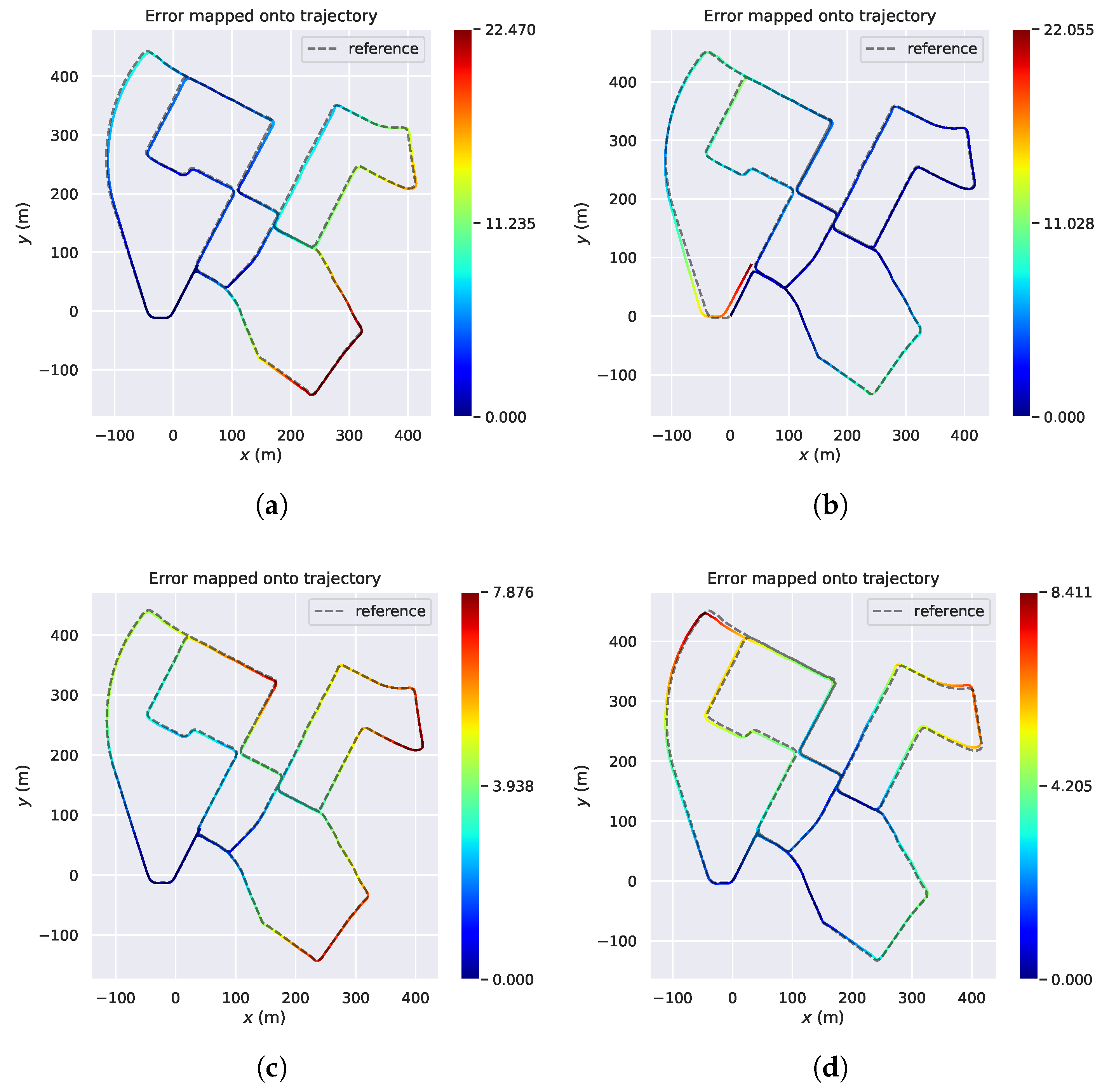
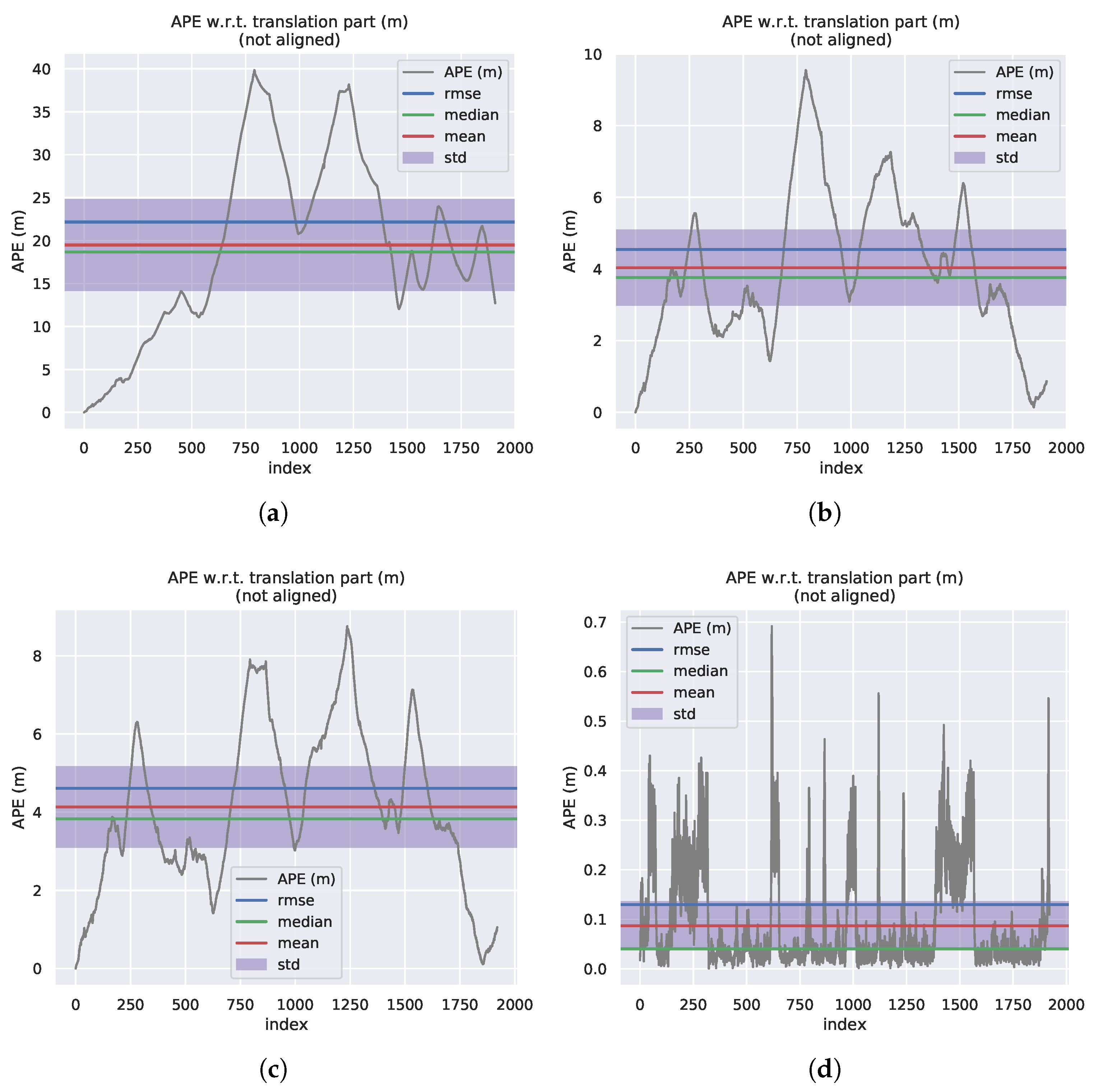
4.1. Accuracy in KITTI Dataset

To illustrate the advantages of the proposed method in an outdoor environment, we conducted experiments on the KITTI dataset. We mainly used 3D point cloud data acquired by the Velodyne HDL-64E lidar system. The trajectory was saved in the KITTI data set format, and the timestamp did not need to be saved, as long as the data to be evaluated corresponded to the ground-truth data one-to-one. In the first experiment, the KITTI dataset was used as the input to the designed SLAM system. The resulting motion trajectories are shown in Figure 8; we compared our scheme with A-LOAM, CT-ICP and HDL-SLAM. For the convenience of the comparison, all experiments were performed on the same experimental platform. The comparison results are shown in Table 1. It can be seen from Figure 8 that the absolute pose errors (abbreviation in uppercase, APE) of A-LOAM, CT-ICP and HDL SLAM were 12.17, 4.54 and 4.61, respectively. It can be seen from the experimental results that the systematic error could be well-controlled in the system proposed in this paper.
The absolute pose error and the relative pose error (abbreviation in uppercase, RPE) are shown in Table 1. It can be seen that the algorithm proposed in this paper had great advantages in both the overall pose error and the relative pose drift. From the motion trajectories in Figure 8, the algorithm proposed in this paper had the smallest gap with the true value.

4.2. Accuracy in M2DGR Dataset

To further demonstrate the robustness of our SLAM system, we conducted experiments in nighttime scenes. The M2DGR dataset contains data collected from multiple nighttime scenes. The absolute pose errors of the motion trajectories of the mobile robot are shown in Figure 9, and the results are recorded in Table 2. It can be seen that our proposed method had the best error control ability. Compared with HDL SLAM, we reduced the relative pose error by 1.72 and the absolute pose error by 1.26. Therefore, our scheme had a good performance in both error control and trajectory offset. The point cloud map was constructed using the M2DGR dataset as shown in Figure 10. Our method was more uniform in the distribution of errors than other algorithms, and the mean and variance of the errors were also minimized.
A-LOAM is an improved version of LOAM that uses the code of LOAM optimized by the Eigen and Ceres libraries. However, as it is only a lidar odometry without loop-closure detection, it cannot be called a SLAM algorithm, so the overall accuracy is poor. The advantage of HDL SLAM lies in the abnormal judgment of the pose during the matching, and some abnormal frames can be discarded. However, when matching, only one point cloud frame is selected as the target point cloud. If the point cloud is too sparse, a large error will be generated. CT-ICP is a new odometry method that ensures the real-time performance of the algorithm, but the back-end optimization is carried out only when loop-closure data are recognized, and the optimization effect is poor for a large scene without loop closure.

5. Conclusions

This paper investigated a SLAM system for mobile robots. To improve the registration accuracy and computation efficiency, a new variant of the NDT algorithm was proposed, which was different from those previously proposed in that it contained a ground-point remover and a point cloud segmentation algorithm. In addition, a loop-closure algorithm included in the depth-completion algorithm made the proposed SLAM system more robust in practical applications. Finally, experimental results were provided to demonstrate the good localization and mapping performance of the proposed SLAM system.

Author Contributions

Writing—original draft preparation, L.Y. and Z.Y.; writing—review, G.L. and C.D.; simulation, Z.Y. All authors have read and agreed to the published version of the manuscript.

Funding

This work was supported by the National Natural Science Foundation of China under grant 61941301, grant 61803090 and grant 11771102, in part by the Natural Science Foundation of Guangdong Province under grants 2019A1515012109, 2021A030310668, 2022A1515010178 and 2022A1515010364, in part by the Science and Technology Foundation of Guangdong Province under grants 2019B090910001 and 2021A0101180005, in part by China Postdoctoral Science Foundation under grant 2018M633353, in part by the Special Program for Key Field of Guangdong Colleges under grant 2019KZDZX1037 and in part by the Scientific and Technical Supporting Programs of Sichuan Province under grant 2019YFG0352.

Institutional Review Board Statement

Not applicable.

Informed Consent Statement

Not applicable.

Data Availability Statement

Not applicable.

Conflicts of Interest

The authors declare no conflict of interest.

References

  1. Akashi, H.; Kumamoto, H. Random sampling approach to state estimation in switching environments. Automatica 1977, 13, 429–434. [Google Scholar] [CrossRef]
  2. Murphy, K.; Russell, S. Rao-Blackwellised Particle Filtering for Dynamic Bayesian Networks; Springer: Berlin/Heidelberg, Germany, 2001; pp. 499–515. [Google Scholar]
  3. Grisetti, G.; Stachniss, C.; Burgard, W. Improved techniques for grid mapping with rao-blackwellized particle filters. IEEE Trans. Robot. 2007, 23, 34–46. [Google Scholar] [CrossRef]
  4. Eliazar, A.; Parr, R. Dp-slam: Fast, robust simultaneous localization and mapping without predetermined landmarks. In Proceedings of the IJCAI, Acapulco, Mexico, 9–15 August 2003; pp. 1135–1142. [Google Scholar]
  5. Choi, K.-S.; Lee, S.-G. Enhanced slam for a mobile robot using extended kalman filter and neural networks. Int. J. Precis. Eng. Manuf. 2010, 11, 255–264. [Google Scholar] [CrossRef]
  6. Huang, G.P.; Mourikis, A.I.; Roumeliotis, S.I. A quadratic-complexity observability-constrained unscented kalman filter for slam. IEEE Trans. Robot. 2013, 29, 1226–1243. [Google Scholar] [CrossRef]
  7. Zhou, H.; Ni, K.; Zhou, Q.; Zhang, T. An SFM algorithm with good convergence that addresses outliers for realizing mono-SLAM. IEEE Trans. Ind. Inform. 2016, 12, 515–523. [Google Scholar] [CrossRef]
  8. Kohlbrecher, S.; Von Stryk, O.; Meyer, J.; Klingauf, U. A flexible and scalable slam system with full 3d motion estimation. In Proceedings of the 2011 IEEE International Symposium on Safety, Security, and Rescue Robotics, Kyoto, Japan, 1–5 November 2011; pp. 155–160. [Google Scholar]
  9. Konolige, K.; Grisetti, G.; Kümmerle, R.; Burgard, W.; Limketkai, B.; Vincent, R. Efficient sparse pose adjustment for 2d mapping. In Proceedings of the 2010 IEEE/RSJ International Conference on Intelligent Robots and Systems, Taipei, Taiwan, 18–22 October 2010; pp. 22–29. [Google Scholar]
  10. Hess, W.; Kohler, D.; Rapp, H.; Andor, D. Real-time loop closure in 2d lidar slam. In Proceedings of the 2016 IEEE International Conference on Robotics and Automation (ICRA), Stockholm, Sweden, 16–21 May 2016; pp. 1271–1278. [Google Scholar]
  11. Besl, P.J.; McKay, N.D. Method for registration of 3-d shapes. Sensor fusion IV: Control paradigms and data structures. Int. Soc. Opt. Photonics 1992, 1611, 586–606. [Google Scholar]
  12. Magnusson, M. The Three-Dimensional Normal-Distributions Transform: An Efficient Representation for Registration, Surface Analysis, and Loop Detection. Ph.D. Thesis, Örebro Universitet, Örebro, Sweden, 2009. [Google Scholar]
  13. Zhang, J.; Singh, S. Loam: Lidar odometry and mapping in real-time. Robot. Sci. Syst. 2014, 2, 1–9. [Google Scholar]
  14. Shan, T.; Englot, B. Lego-loam: Lightweight and ground-optimized lidar odometry and mapping on variable terrain. In Proceedings of the 2018 IEEE/RSJ International Conference on Intelligent Robots and Systems (IROS), Madrid, Spain, 1–5 October 2018; pp. 4758–4765. [Google Scholar]
  15. Gao, H.; Zhang, X.; Wen, J.; Yuan, J.; Fang, Y. Autonomous indoor exploration via polygon map construction and graph-based slam using directional endpoint features. IEEE Trans. Autom. Sci. Eng. 2018, 16, 1531–1542. [Google Scholar] [CrossRef]
  16. Jung, S.; Choi, D.; Song, S.; Myung, H. Bridge inspection using unmanned aerial vehicle based on hg-slam: Hierarchical graph-based slam. Remote Sens. 2020, 12, 3022. [Google Scholar] [CrossRef]
  17. Lin, J.; Zheng, C.; Xu, W.; Zhang, F. R2live: A robust, real-time, lidar-inertial-visual tightly-coupled state estimator and mapping. IEEE Robot. Autom. Lett. 2021, 6, 7469–7476. [Google Scholar] [CrossRef]
  18. Segal, A.; Haehnel, D.; Thrun, S. Generalized-icp. Robot. Sci. Syst. 2009, 2, 435. [Google Scholar]
  19. Serafin, J.; Grisetti, G. Nicp: Dense normal based point cloud registration. In Proceedings of the 2015 IEEE/RSJ International Conference on Intelligent Robots and Systems (IROS), Hamburg, Germany, 28 September–3 October 2015; pp. 742–749. [Google Scholar]
  20. Hong, H.; Lee, B. Dynamic scaling factors of covariances for accurate 3d normal distributions transform registration. In Proceedings of the 2018 IEEE/RSJ International Conference on Intelligent Robots and Systems (IROS), Madrid, Spain, 1–5 October 2018; pp. 1190–1196. [Google Scholar]
  21. Zaganidis, A.; Magnusson, M.; Duckett, T.; Cielniak, G. Semantic-assisted 3d normal distributions transform for scan registration in environments with limited structure. In Proceedings of the 2017 IEEE/RSJ International Conference on Intelligent Robots and Systems (IROS), Vancouver, BC, Canada, 24–28 September 2017; pp. 4064–4069. [Google Scholar]
  22. Schulz, C.; Zell, A. Real-time graph-based slam with occupancy normal distributions transforms. In Proceedings of the 2020 IEEE International Conference on Robotics and Automation (ICRA), Paris, France, 31 May–31 August 2020; pp. 3106–3111. [Google Scholar]
  23. Rusinkiewicz, S.; Levoy, M. Efficient variants of the icp algorithm. In Proceedings of the Third International Conference on 3-D Digital Imaging and Modeling, Quebec City, QC, Canada, 28 May–1 June 2001; pp. 145–152. [Google Scholar]
  24. Kim, G.; Kim, A. Scan context: Egocentric spatial descriptor for place recognition within 3d point cloud map. In Proceedings of the 2018 IEEE/RSJ International Conference on Intelligent Robots and Systems (IROS), Madrid, Spain, 1–5 October 2018; pp. 4802–4809. [Google Scholar]
  25. Wang, H.; Wang, C.; Xie, L. Intensity scan context: Coding intensity and geometry relations for loop closure detection. In Proceedings of the 2020 IEEE International Conference on Robotics and Automation (ICRA), Paris, France, 31 May–31 August 2020; pp. 2095–2101. [Google Scholar]
  26. Wang, Y.; Sun, Z.; Xu, C.Z.; Sarma, S.E.; Yang, J.; Kong, H. Lidar iris for loop-closure detection. In Proceedings of the 2020 IEEE/RSJ International Conference on Intelligent Robots and Systems (IROS), Las Vegas, NV, USA, 24 October–24 January 2021; pp. 5769–5775. [Google Scholar]
  27. Gálvez-López, D.; Tardos, J.D. Bags of binary words for fast place recognition in image sequences. IEEE Trans. Robot. 2012, 28, 1188–1197. [Google Scholar] [CrossRef]
  28. Suger, B.; Tipaldi, G.D.; Spinello, L.; Burgard, W. An approach to solving large-scale slam problems with a small memory footprint. In Proceedings of the 2014 IEEE International Conference on Robotics and Automation (ICRA), Hong Kong, China, 31 May–7 June 2014; pp. 3632–3637. [Google Scholar]
  29. Chen, P.; Peng, Y.; Wang, S. The Hessian matrix of Lagrange function. Linear Algebra Its Appl. 2017, 531, 537–546. [Google Scholar] [CrossRef]
  30. Hu, M.; Wang, S.; Li, B.; Ning, S.; Fan, L.; Gong, X. Penet: Towards precise and efficient image guided depth completion. In Proceedings of the 2021 IEEE International Conference on Robotics and Automation (ICRA), Xi’an, China, 30 May–5 June 2021; pp. 13656–13662. [Google Scholar]
  31. Geiger, A.; Lenz, P.; Urtasun, R. Are we ready for autonomous driving? The kitti vision benchmark suite. In Proceedings of the 2012 IEEE Conference on Computer Vision and Pattern Recognition, Providence, RI, USA, 16–21 June 2012; pp. 3354–3361. [Google Scholar]
  32. Yin, J.; Li, A.; Li, T.; Yu, W.; Zou, D. M2dgr: A multi-sensor and multi-scenario slam dataset for ground robots. IEEE Robot. Autom. Lett. 2021, 7, 2266–2273. [Google Scholar] [CrossRef]
Figure 1. An overview of the SLAM algorithm proposed in this paper.
Mathematics 11 02211 g001
Figure 2. Using a ground segmentation algorithm to remove useless ground points.
Mathematics 11 02211 g002
Figure 3. Assuming that the sensor is located at O, and the lines O A and O B represent two laser beams, points A and B produce a line to estimate the surface of the object (if they all belong to the same object).
Mathematics 11 02211 g003
Figure 4. Region segmentation using point cloud spatial distribution characteristics and local adjacency relationship, different colors represent point clouds divided into different subspaces. (The more dark the color, the more dense feature points).
Mathematics 11 02211 g004
Figure 5. Using the matching algorithm proposed in this section to register the two frames’ point clouds.
Mathematics 11 02211 g005
Figure 6. Projecting the point cloud data into the image space. (a) The relationship between the various coordinate systems; (b) the projected result.
Mathematics 11 02211 g006
Figure 7. Converting a sparse depth image and an RGB image to a dense depth image using PENet. (a) RGB image; (b) sparse depth image; (c) dense depth image.
Mathematics 11 02211 g007
Figure 8. Motion trajectories obtained using different loop-closure detection algorithms in the KITTI dataset. (a) A-LOAM; (b) CT-ICP; (c) HDL SLAM; (d) ours.
Mathematics 11 02211 g008
Figure 9. APE curves obtained using different SLAM algorithms in the M2DGR dataset. (a) A-LOAM; (b) CT-ICP; (c) HDL SLAM; (d) ours.
Mathematics 11 02211 g009
Figure 10. The point cloud map of the M2DGR dataset constructed using the SLAM algorithm proposed in this paper.
Mathematics 11 02211 g010
Table 1. Comparison of trajectory accuracy obtained by different SLAM algorithms under the KITTI dataset.
A-LOAMCT-ICPHDL SLAMOurs
APE(m)12.1714034.5425284.6120942.029666
RPE(%)2.5126802.3191011.8194291.786136
Table 2. Comparison of trajectory accuracy obtained by different SLAM algorithms under the M2DGR dataset.
A-LOAMCT-ICPHDL SLAMOurs
APE(m)8.3821804.0440643.4479701.725925
RPE(%)3.0696322.8551112.7259251.469667
Disclaimer/Publisher’s Note: The statements, opinions and data contained in all publications are solely those of the individual author(s) and contributor(s) and not of MDPI and/or the editor(s). MDPI and/or the editor(s) disclaim responsibility for any injury to people or property resulting from any ideas, methods, instructions or products referred to in the content.

