
On Targeted Control over Trajectories of Dynamical Systems Arising in Models of Complex Networks


Abstract
:1. Introduction
2. GRN System
3. Description of the State Space for System (2)
3.1. Attractors
3.2. Influence of Parameters on the Structure of the Phase Plane of 2D GRN Systems
- There is an invariant set with the following properties:
- 1a
- The vector field defined by the system (8) is directed inward on the border of
- 1b
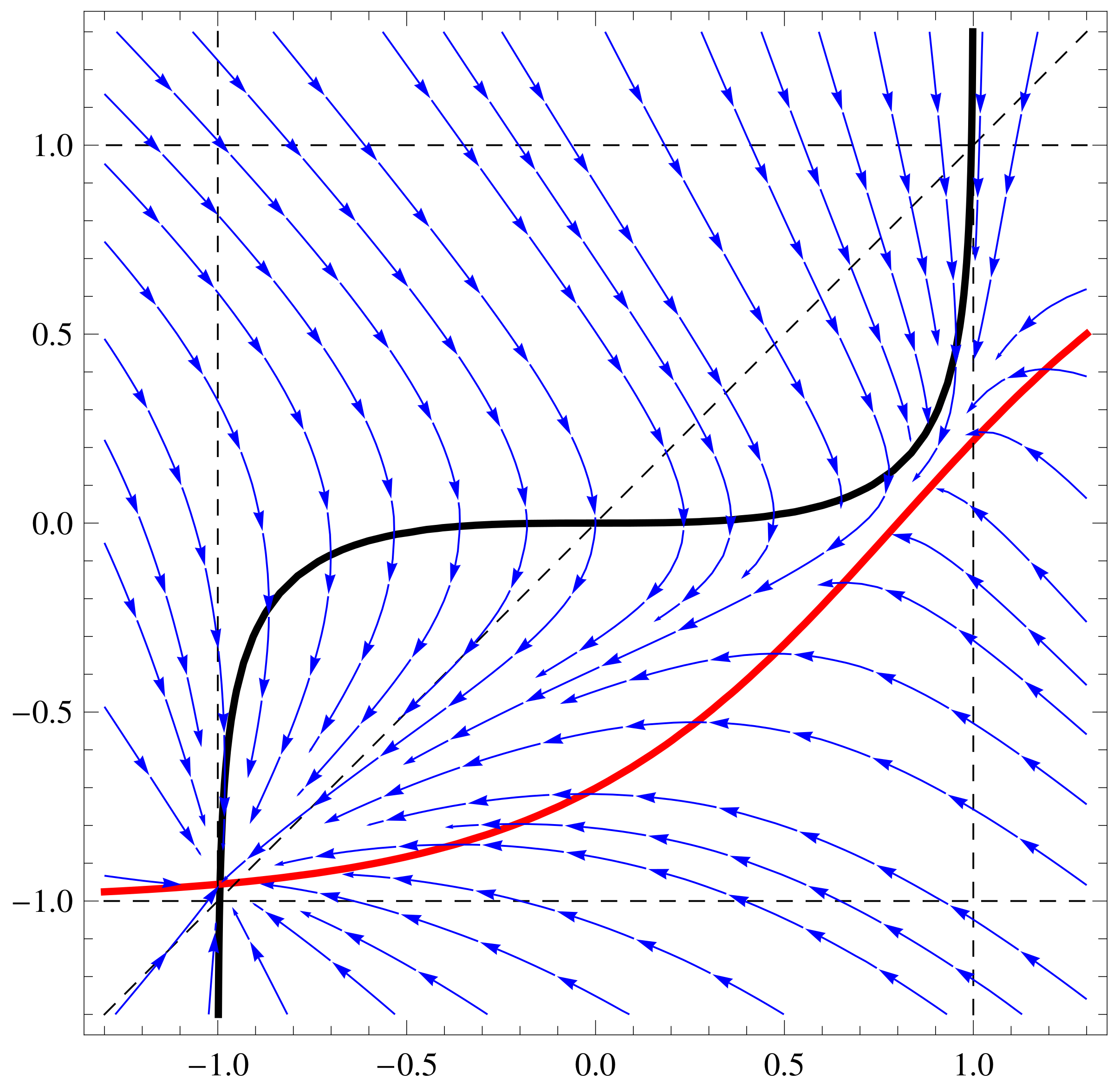
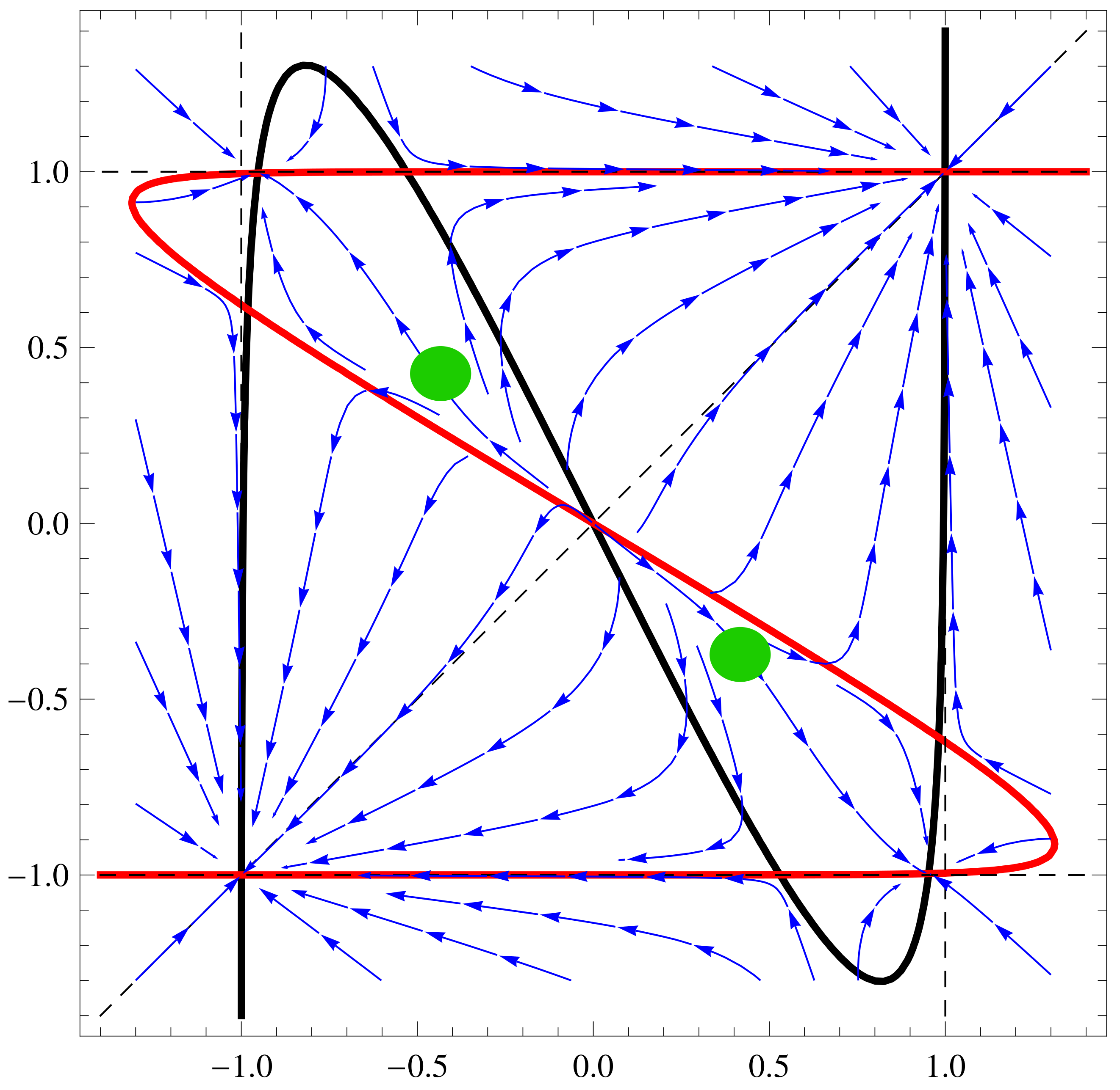
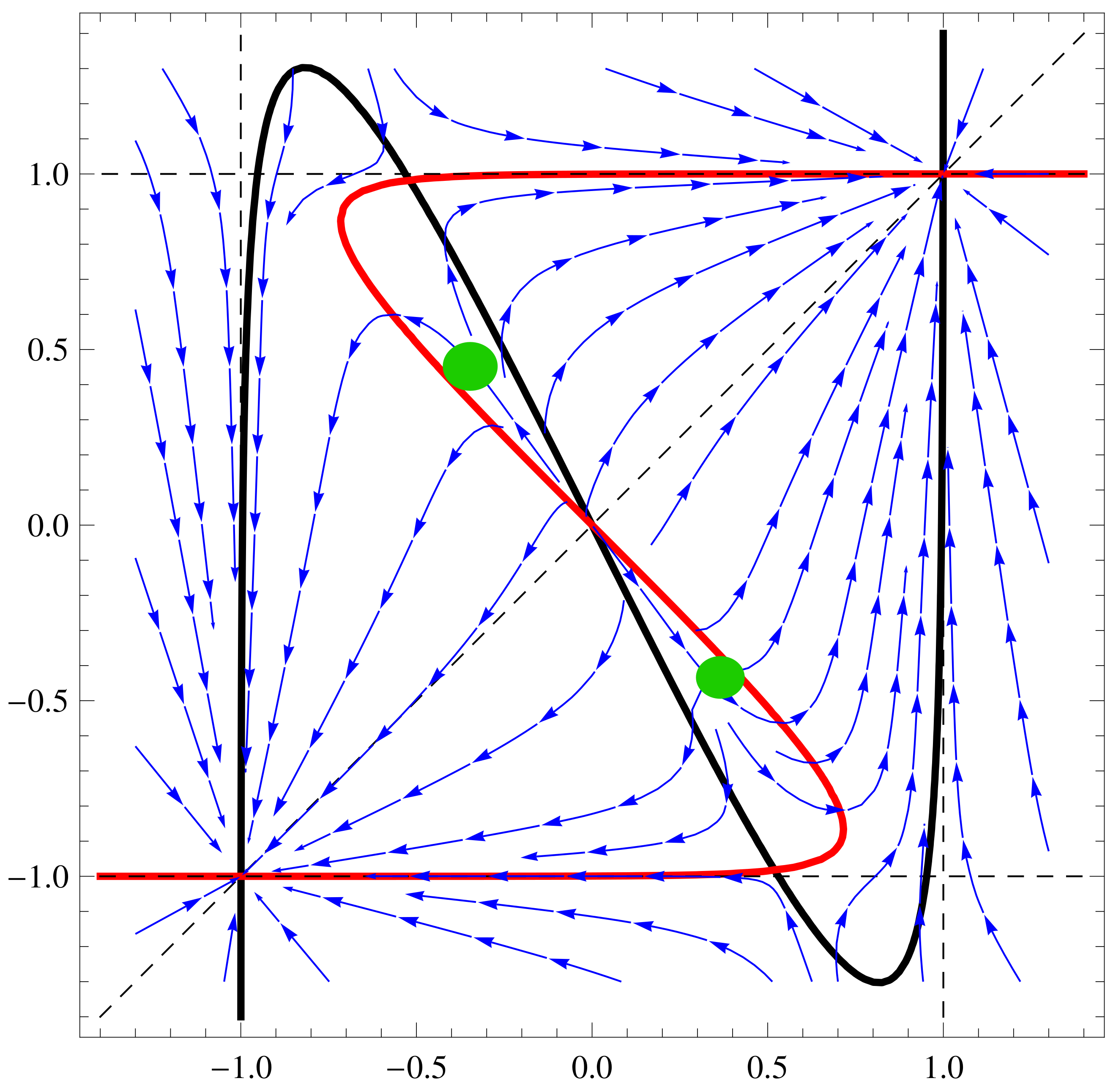
- The nullclines (9) can intersect only in
- 1c
- The nullclines intersect at least once. The total number of intersections is finite. For the 2D case, the maximal number of critical points is nine. For this, both nullclines have to be Z-shaped;
- By changing , the nullclines can be shifted; by changing , the first nullcline can be shifted in the vertical direction; by changing , the second nullcline is moved horizontally, preserving shape;
- By changing , the shapes of the nullclines can be changed; for sufficiently large values of , the three segments of a sigmoid curve, representing a nullcline, become almost straight. In this case, the system (8) is almost piece-wise linear; for the study of the case of piece-wise linear system consult [24];
- By changing , the parallelepiped can be made stretched or compressed; for , it is a unit square;
- Signs of elements of the regulatory matrixare of great importance. The typical cases are
- 5a
- Activation: , , , ;
- 5b
- Inhibition: , ,
- 5c
- Mixed: , , ;
3.3. Inhibition Case in 2D GRN Systems
3.4. Controllability by Changing
3.5. Controllability by Changing Both
4. Driving the System from One State to Another One—ANN Case
Controllability by Changing an Element of A
5. Conclusions
Author Contributions
Funding
Data Availability Statement
Acknowledgments
Conflicts of Interest
Appendix A
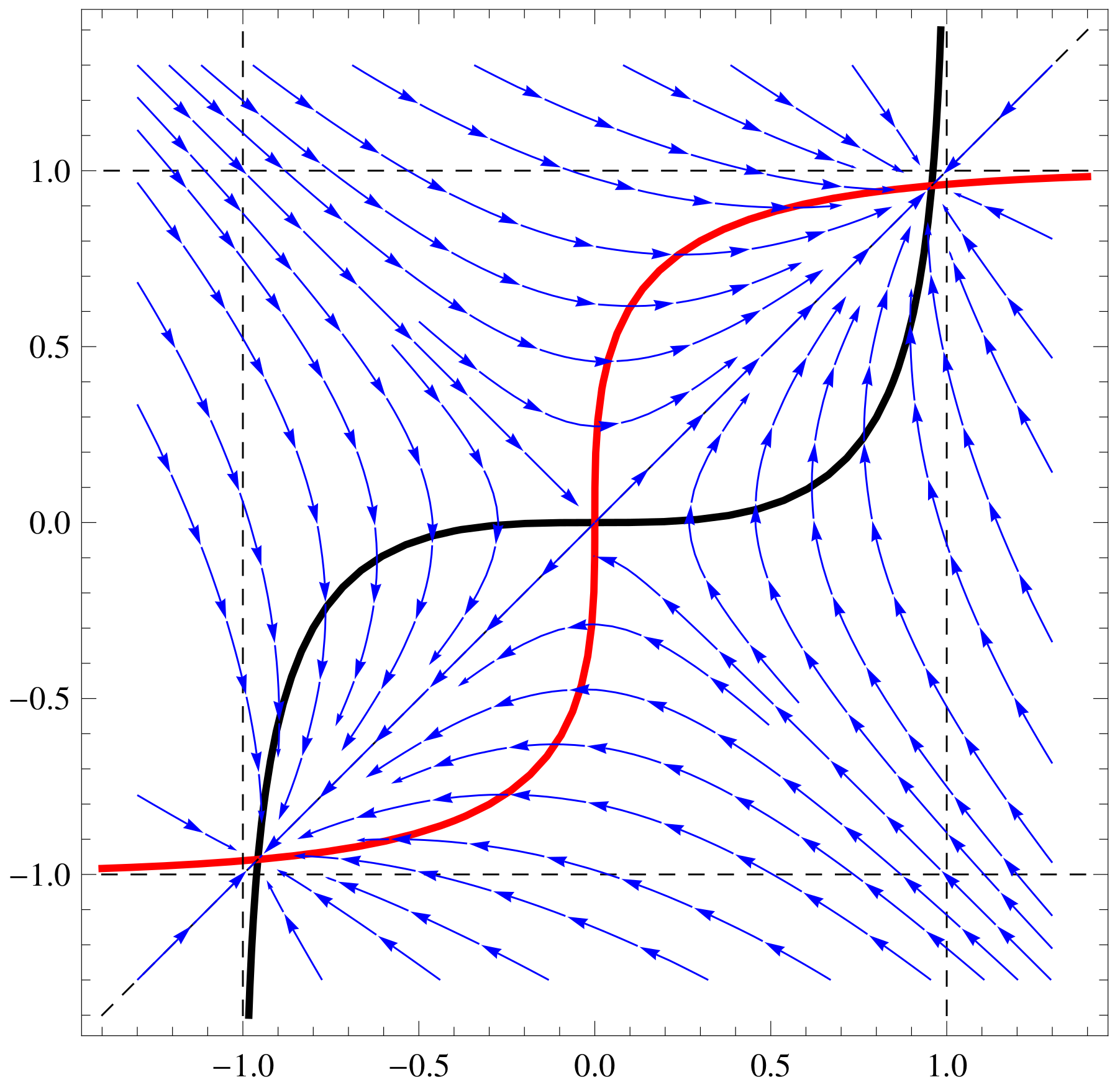
a11=1;a12=1;a21=1;a22=1;b1=1;b2=1; f1[x_,y_]:=Tanh[a11 x+a12 y]-b1
x; f2[x_,y_]:=Tanh[a21 x+a22 y]-b2 y;
ContourPlot[{f1[x,y]==0,f2[x,y]==0,x==y, x==1, x==-1, y==1,
y==-1},{x,-1.4,1.4},{y,-1.4,1.4},ContourStyle->
{{Thick,Black},{Thick,Red},Dashed, Dashed, Dashed, Dashed,
Dashed},AxesLabel-> {Style[x,15],Style[y,15]}]
a11=1;a12=1;a21=5;a22=-5;b1=1;b2=1;
ContourPlot[{f1[x,y]==0,f2[x,y]==0,x==y, x==1, x==-1, y==1,
y==-1},{x,-1.4,1.4},{y,-1.4,1.4},ContourStyle->
{{Thick,Black},{Thick,Red},Dashed, Dashed, Dashed, Dashed,
Dashed},AxesLabel-> {Style[x,15],Style[y,15]}]
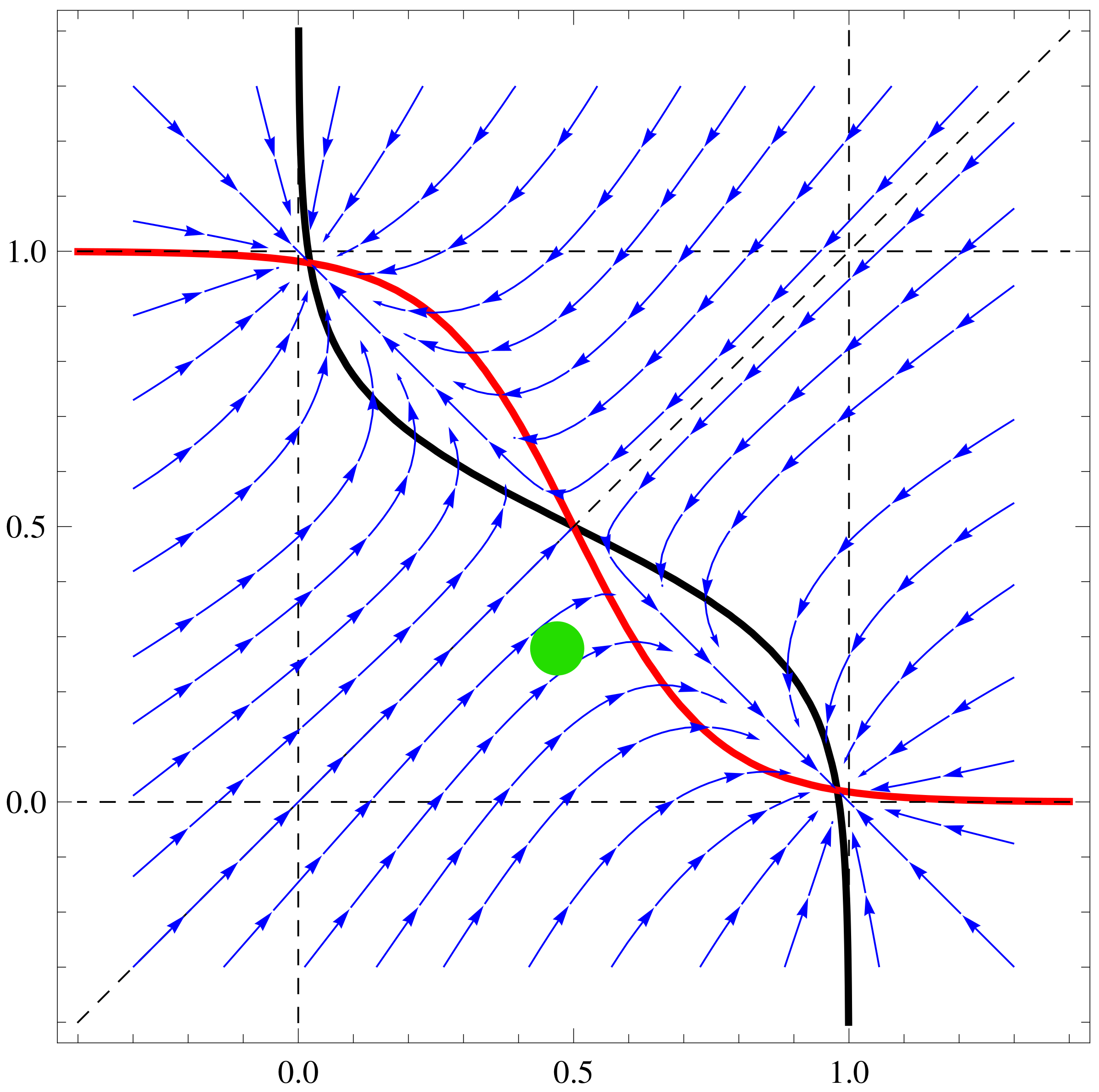
Clear[x,y];
a11=1;a12=2;a21=1;a22=0.1;b1=1;b2=1;\[CapitalTheta]1=0.1;
\[CapitalTheta]2=0.8;
\[Mu]1=1; \[Mu]2=1; f1[x_,y_]:=Tanh[\[Mu]1 (a11 x+a12
y-\[CapitalTheta]1)]-b1 x; f2[x_,y_]:=Tanh[\[Mu]2 (a21 x+a22
y-\[CapitalTheta]2)]-b2 y;
nc2=ContourPlot[{f1[x,y]==0,f2[x,y]==0,x==y,x==1, x==-1, y==1,
y==-1},{x,-1.3,1.3},{y,-1.3,1.3},ContourStyle->
{{Thick,Black},{Thick,Red},Dashed,Dashed,Dashed,Dashed,Dashed},
AxesLabel->{Style[x,15],Style[y,15]}]
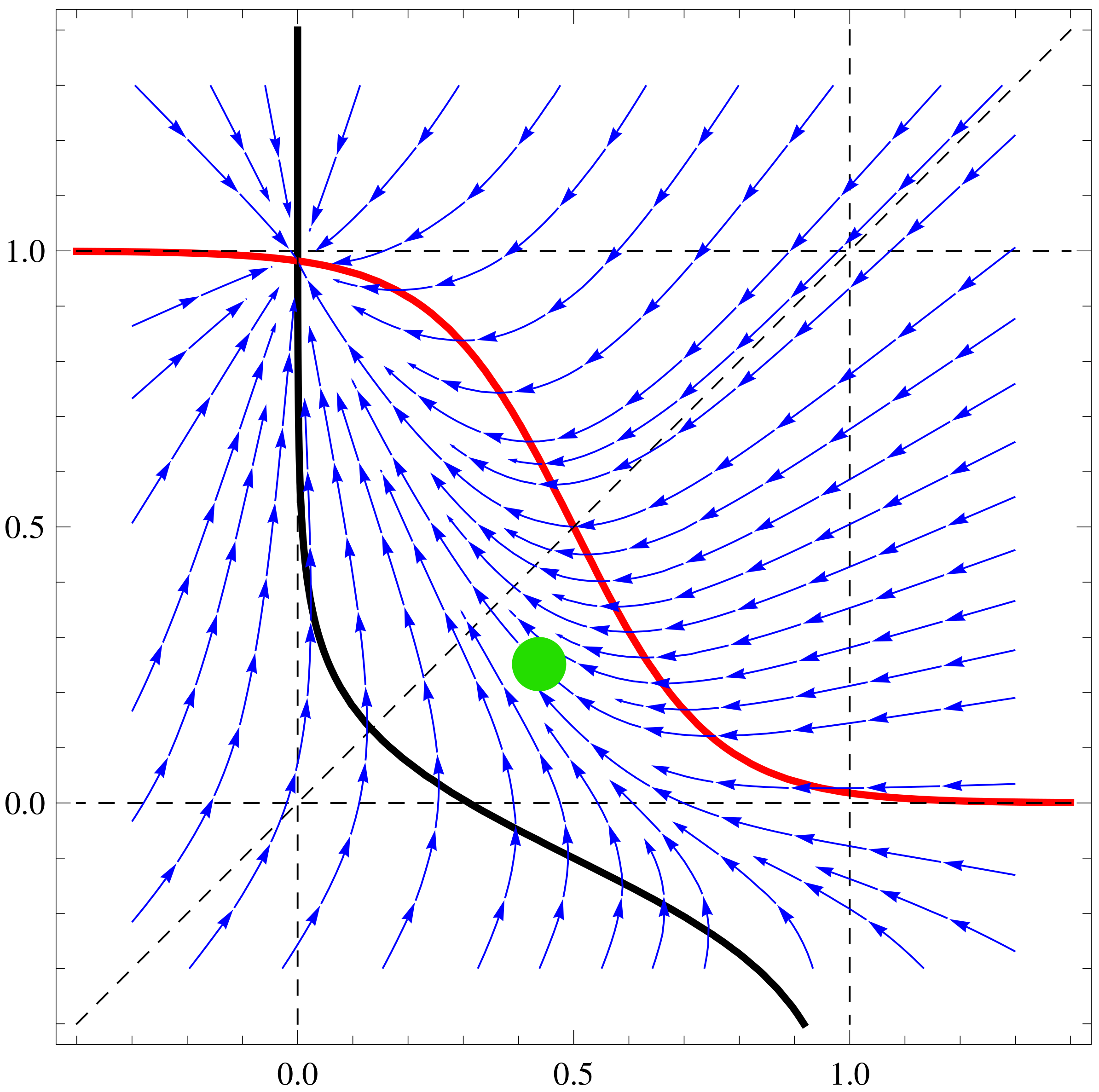
a11=3;a12=1;a21=3;a22=6;b1=1;b2=1; f1[x_,y_]:=Tanh[a11 x+a12 y]-b1
x; f2[x_,y_]:=Tanh[a21 x+a22 y]-b2 y;
nc1=ContourPlot[{f1[x,y]==0,f2[x,y]==0,x==y, x==1, x==-1, y==1,
y==-1},{x,-1.4,1.4},{y,-1.4,1.4},ContourStyle->
{{Thick,Black},{Thick,Red},Dashed, Dashed, Dashed, Dashed,
Dashed},AxesLabel-> {Style[x,15],Style[y,15]}]
sp1=StreamPlot[{ f1[x,y], f2[x,y]}, {x, -1.3, 1.3}, {y, -1.3, 1.3},
Axes -> True, Frame->True, AxesLabel -> {Style["x",Black, FontSize->
16],Style["y",Black,Italic,FontSize-> 16]}, StreamPoints ->40,
StreamStyle-> {Blue}]
Show[nc1, sp1]
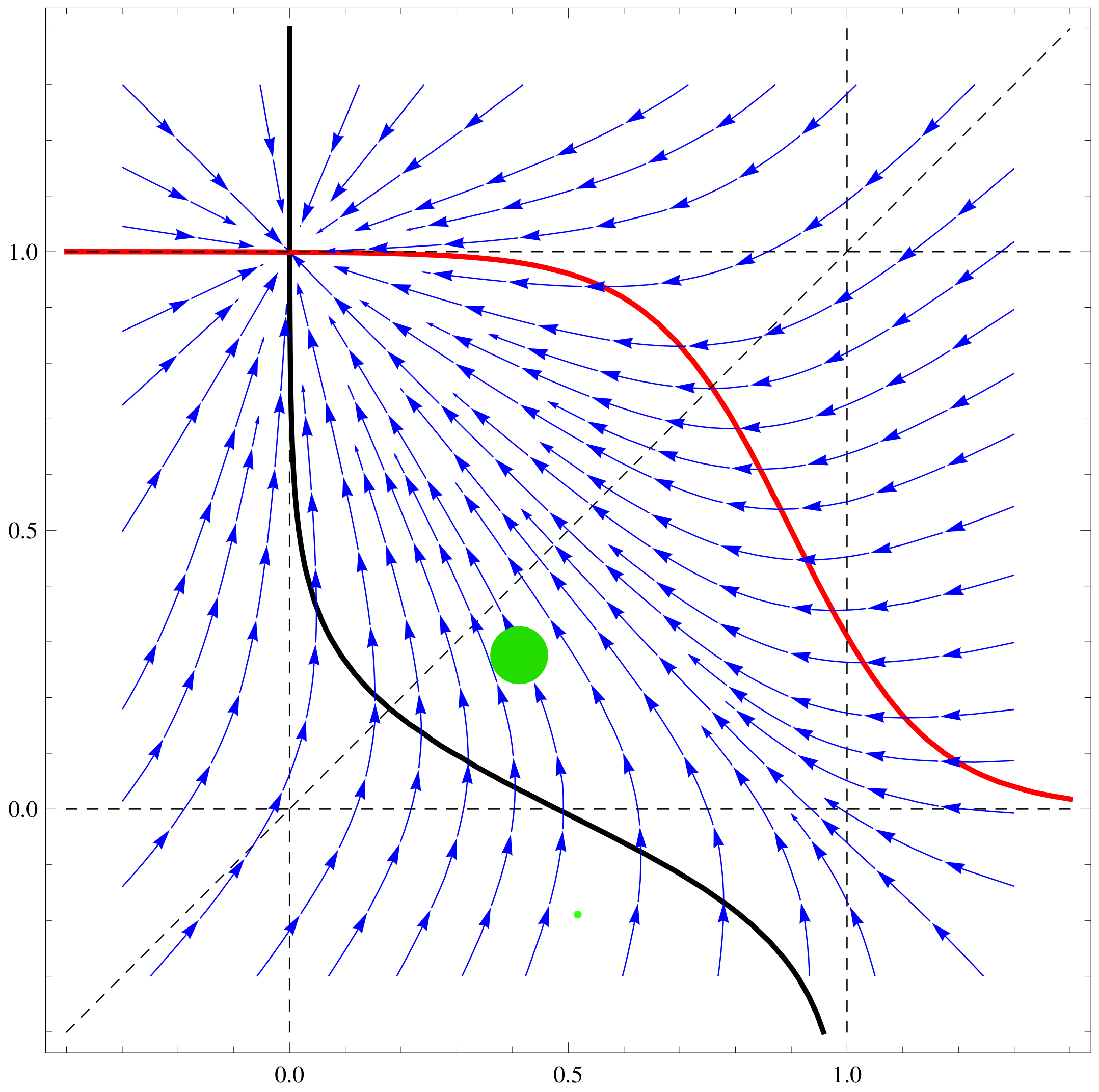
a11=3;a12=1;a21=3;a22=4;b1=1;b2=1; f1[x_,y_]:=Tanh[a11 x+a12 y]-b1
x; f2[x_,y_]:=Tanh[a21 x+a22 y]-b2 y;
nc2=ContourPlot[{f1[x,y]==0,f2[x,y]==0,x==y, x==1, x==-1, y==1,
y==-1},{x,-1.4,1.4},{y,-1.4,1.4},ContourStyle->
{{Thick,Black},{Thick,Red},Dashed, Dashed, Dashed, Dashed,
Dashed},AxesLabel-> {Style[x,15],Style[y,15]}]
sp2=StreamPlot[{ f1[x,y], f2[x,y]}, {x, -1.3, 1.3}, {y, -1.3, 1.3},
Axes -> True, Frame->True, AxesLabel -> {Style["x",Black, FontSize->
16],Style["y",Black,Italic,FontSize-> 16]}, StreamPoints ->40,
StreamStyle-> {Blue}]
Show[nc2, sp2]
References
- Sayama, H. Introduction to the Modeling and Analysis of Complex Systems. Milne Open Textbooks. 14. 2015. Available online: https://knightscholar.geneseo.edu/oer-ost/14 (accessed on 14 February 2023).
- De Jong, H. Modeling and Simulation of Genetic Regulatory Systems: A Literature Review. J. Comput. Biol. 2002, 9, 67–103. [Google Scholar] [CrossRef] [PubMed]
- Brokan, E.; Sadyrbaev, F.Z. On controllability of nonlinear dynamical network. AIP Conf. Proc. 2019, 2116, 040005. [Google Scholar] [CrossRef]
- Koizumi, Y.; Miyamura, T.; Arakawa, S.I.; Oki, E.; Shiomoto, K.; Murata, M. Adaptive Virtual Network Topology Control Based on Attractor Selection. J. Light. Technol. 2010, 28, 1720–1731. [Google Scholar] [CrossRef]
- Furusawa, C.; Kaneko, K. A generic mechanism for adaptive growth rate regulation. PLoS Comput. Biol. 2008, 4, e3. [Google Scholar] [CrossRef]
- Cornelius, S.P.; Kath, W.L.; Motter, A.E. Realistic control of network dynamic. Nat. Commun. 2013, 4, 1942. [Google Scholar] [CrossRef]
- Wang, L.-Z.; Su, R.-Q.; Huang, Z.-G.; Wang, X.; Wang, W.-X.; Grebogi, C.; Lai, Y.-C. A geometrical approach to control and controllability of nonlinear dynamical networks. Nat. Commun. 2016, 7, 11323. [Google Scholar] [CrossRef]
- Samuilik, I.; Sadyrbaev, F. On trajectories of a system modeling evolution of genetic networks. Math. Eng. 2023, 20, 2232–2242. [Google Scholar] [CrossRef]
- Barabási, A.-L.; Oltvai, Z.N. Network biology: Understanding the cell’s functional organization. Nat. Rev. Genet. 2004, 5, 101–113. [Google Scholar] [CrossRef]
- Dehmamy, N.; Milanlouei, S.; Barabási, A.-L. A structural transition in physical networks. Nature 2018, 563, 676–680. [Google Scholar] [CrossRef]
- Liu, Y.-Y.; Slotine, J.-J.; Barabási, A.-L. Observability of complex systems. Proc. Natl. Acad. Sci. USA 2013, 110, 2460–2465. [Google Scholar] [CrossRef]
- Liu, Y.-Y.; Slotine, J.-J.; Barabási, A.-L. Controllability of complex networks. Nature 2011, 473, 167–173. [Google Scholar] [CrossRef] [PubMed]
- Slotine, J.J.; Li, W. Applied Nonlinear Control; Prentice Hall: Hoboken, NJ, USA, 1991. [Google Scholar]
- Sadyrbaev, F.; Samuilik, I.; Sengileyev, V. On modelling of genetic regulatory networks. WSEAS Trans. Electron. 2021, 12, 72–80. [Google Scholar] [CrossRef]
- Samuilik, I.; Sadyrbaev, F. On a dynamical model of genetic networks. WSEAS Trans. Bus. Econ. 2023, 20, 104–112. [Google Scholar] [CrossRef]
- Brokan, E.; Sadyrbaev, F.Z. On Attractors in Gene Regulatory Systems. AIP Conf. Proc. 2017, 1809, 020010. [Google Scholar] [CrossRef]
- Brokan, E.; Sadyrbaev, F. Attraction in n-dimensional differential systems from network regulation theory. Math. Methods Appl. Sci. 2018, 41, 7498–7509. [Google Scholar] [CrossRef]
- Brokan, E.; Sadyrbaev, F. On a differential system arising in the network control theory. Nonlinear Anal. Model. Control 2016, 21, 5. [Google Scholar] [CrossRef]
- Ogorelova, D.; Sadyrbaev, F.; Sengileyev, V. Control in inhibitory genetic regulatory networks. Contemp. Math. 2020, 1, 393–400. [Google Scholar] [CrossRef]
- Vinayagama, A.; Gibsonb, T.E.; Lee, H.-J.; Yilmazeld, B.; Roeseld, C.; Hua, Y.; Kwona, Y.; Sharma, A.; Liu, Y.-Y.; Perrimona, N.; et al. Controllability Analysis of the Directed Human Protein Interaction Network Identifies Disease Genes and Drug Targets. Proc. Natl. Acad. Sci. USA 2016, 113, 4976–4981. [Google Scholar] [CrossRef]
- Vohradský, J. Neural network model of gene expression. FASEB J. 2001, 15, 846–854. [Google Scholar] [CrossRef]
- Wuensche, A. Genomic regulation modeled as a network with basins of attraction. Proc. Pac. Symp. Biocomput. 1998, 3, 89–102. [Google Scholar]
- Wilson, H.R.; Cowan, J.D. Excitatory and inhibitory interactions in localized populations of model neurons. Biophys. J. 1972, 12, 1–24. [Google Scholar] [CrossRef] [PubMed]
- Edwards, R.; Ironi, L. Periodic solutions of gene networks with steep sigmoidal regulatory functions. Physic D 2014, 282, 1–15. [Google Scholar] [CrossRef]
- Sadyrbaev, F. Planar differential systems arising in network regulation theory. Adv. Math. Model. Appl. 2019, 4, 70–78. [Google Scholar]
- Kozlovska, O.; Sadyrbaev, F. Models of genetic networks with given properties. WSEAS Trans. Comp. Res. 2022, 10, 43–49. [Google Scholar] [CrossRef]
- Sprott, J.C. Elegant Chaos: Algebraically Simple Chaotic Flow; World Scientific: Singapore, 2010. [Google Scholar]
- Iglesias, P.A.; Ingalls, B.P. (Eds.) Control Theory and Systems Biology; MIT Press: Cambridge, MA, USA; London, UK, 2010. [Google Scholar]


Disclaimer/Publisher’s Note: The statements, opinions and data contained in all publications are solely those of the individual author(s) and contributor(s) and not of MDPI and/or the editor(s). MDPI and/or the editor(s) disclaim responsibility for any injury to people or property resulting from any ideas, methods, instructions or products referred to in the content. |
© 2023 by the authors. Licensee MDPI, Basel, Switzerland. This article is an open access article distributed under the terms and conditions of the Creative Commons Attribution (CC BY) license (https://creativecommons.org/licenses/by/4.0/).
Share and Cite
Ogorelova, D.; Sadyrbaev, F.; Samuilik, I. On Targeted Control over Trajectories of Dynamical Systems Arising in Models of Complex Networks. Mathematics 2023, 11, 2206. https://doi.org/10.3390/math11092206
Ogorelova D, Sadyrbaev F, Samuilik I. On Targeted Control over Trajectories of Dynamical Systems Arising in Models of Complex Networks. Mathematics. 2023; 11(9):2206. https://doi.org/10.3390/math11092206
Chicago/Turabian StyleOgorelova, Diana, Felix Sadyrbaev, and Inna Samuilik. 2023. "On Targeted Control over Trajectories of Dynamical Systems Arising in Models of Complex Networks" Mathematics 11, no. 9: 2206. https://doi.org/10.3390/math11092206