Article

Dynamics in the Reduced Mean-Field Model of Neuron–Glial Interaction

by
Sergey M. Olenin
,
Tatiana A. Levanova
* and
Sergey V. Stasenko
*
Control Theory Department, Institute of Information Technologies, Mathematics and Mechanics, Lobachevsky State University of Nizhny Novgorod, Nizhny Novgorod 603022, Russia
*
Authors to whom correspondence should be addressed.
Mathematics 2023, 11(9), 2143; https://doi.org/10.3390/math11092143
Submission received: 31 March 2023 / Revised: 24 April 2023 / Accepted: 1 May 2023 / Published: 3 May 2023

Abstract

:
The goal of this study is to propose a new reduced phenomenological model that describes the mean-field dynamics arising from neuron–glial interaction, taking into account short-term synaptic plasticity and recurrent connections in the presence of astrocytic modulation of the synaptic connection. Using computer simulation and numerical methods of nonlinear dynamics, it is shown that the proposed model reproduces a rich set of patterns of population activity, including spiking, bursting and chaotic temporal patterns. These patterns can coexist for specific regions in the parameter space of the model. The main focus of this study was on bifurcation mechanisms that lead to the occurrence of the described types of mean-field dynamics. The proposed phenomenological model can be used to reproduce various patterns of population activity of neurons in a wide range of studies of dynamic memory and information processing. One of the possible applications of such research is the development of new effective methods for the treatment of neurological diseases associated with neuron–glial interactions.

1. Introduction

The study of the synchronization of neural activity in the brain is one of the key directions in modern neurobiology and neurodynamics. In a healthy brain, cognitive processes require the precise integration of neural activity at specific spatiotemporal scales [1,2]. Changes in patterns of synchronous population activity can be observed in some neurological and psychiatric disorders [2].
One of the most interesting and important patterns of synchronous population activity is bursting activity, which is involved in many informational and physiological processes: restoration of synaptic transmission after its disruption [3], release of a neurotransmitter [3], formation of long-term potentiation [3], selectivity of synaptic communication [4], encoding of sensory inputs and increasing information capacity [5,6,7,8,9,10], and many others. It also can underlie pathophysiological processes, e.g., epilepsy [11,12].
Epilepsy affects more than 50 million people worldwide; that is approximately 1 % of the world’s population [13]. The epileptic process is characterized by high spatial and temporal variability [14]. Various biological changes that occur during epileptogenesis are currently described, including neurodegeneration [15], axonal and dendritic plasticity, structural and functional changes in receptors, ion channels, transporters, and enzymes involved in excitatory and inhibitory neurotransmission [16], reorganization of the extracellular matrix [17], and others. These changes may differ qualitatively and quantitatively depending on the triggering event. While most epilepsy research has focused on the intrinsic properties of neurons and the function of the neural network, evidence for a non-neural contribution to epilepsy has increasingly emerged over the past two decades [18,19]. Data show that neuron-surrounding cells, such as astrocytes, microglia and the extracellular matrix can be critically altered in epilepsy [20,21,22] and even be involved in the etiology of the disease. However, this requires more careful study. Recent studies also show that the infection of astrocytes with the COVID-19 virus can lead to impaired physiological processes and brain functions [23,24,25].
Previously, it was shown in a wide range of studies that glial cells are involved in the regulation of synaptic dynamics, see [26,27,28,29,30]. On the basis of these data, a hypothesis of the so-called tripartite synapse was put forward [31]. According to this concept, in addition to the ‘bipartite’ information transfer between the pre- and postsynaptic neurons, astrocytes exchange information with the synaptic neuronal elements, responding to synaptic activity and, in turn, regulating synaptic transmission. Specifically, a neurotransmitter can reach metabotropic glutamate receptors on the surface of the astrocyte membrane, leading to their activation and the subsequent release of gliotransmitters. The gliotransmitter, in its turn, can change the probability of neurotransmitter release by the presynaptic neuron. Thus, a feedback loop is formed [32].
The mechanisms for the formation of synchronous population activity can be explained using mathematical models [33,34]; the most interesting of them is taking into account astrocytic modulation of neuronal activity [35,36,37,38,39]. Thus, such models can shed light on information processing systems [40,41,42] and help to develop methods and approaches for epilepsy treatment [43] through targeted physiological effects on astrocytic dynamics [44].
In this paper, we propose a new phenomenological mathematical model that describes the population dynamics of neurons. The proposed model is based on the Tsodyks–Markram [45] model and takes into account the main features of the neuron–glial interaction through a tripartite synapse. The presented model is a simplification of the previously proposed model [36]. The main attention in our study is given to scenarios for the emergence of complex patterns of population activity. In particular, it has been demonstrated that facilitation of synaptic communication by astrocytes can lead to bursting activity. We also investigate the regions of multistability of different types of dynamics that are observed for the proposed model. The obtained results will help to contribute to the understanding of the complex dynamics of neural networks and become the basis for the development of models of brain pathologies (for example, epileptogenesis), as well as models that describe the functional states of the brain in the process of information processing, learning and memory.

2. The Model

The simplified phenomenological model we propose is based on the Wilson–Cowan [46] model, which describes the dynamics of the excitatory and inhibitory populations of neurons, and the Tsodyks–Markram [47] model of short-term synaptic plasticity, which can be written as a three-dimensional ODE system of the following form:
τ E ˙ = E + α ln 1 + exp J u x E + I 0 α , x ˙ = 1 x τ D u x E , u ˙ = U u τ F + U ( 1 u ) E ,
Here, E ( t ) is the average neuronal activity of the excitatory population (in Hz), J is the strength of recurrent connections, and τ is the time constant of the rate dynamics. Parameter I 0 specifies the inhibitory action from the recurrent network E ( t ) . The parameter α determines the threshold for increasing the average activity of neurons in the excitatory population.
The variable x ( t ) models the amount of available neurotransmitter (glutamate). Presynaptic resources are finite, and each of them can be both available and unavailable for release. The total fraction of the available neurotransmitter is x ( t ) , and the fraction of the inaccessible neurotransmitter is ( 1 x ( t ) ) . The neurotransmitter is consumed in case of the presence of network activity E ( t ) > 0 , which, in turn, leads to short-term synaptic depression. The parameter τ D specifies the characteristic time of synaptic depression.
The variable u ( t ) describes the change in the probability of neurotransmitter release from the presynaptic terminal. The fraction 1 u ( t ) has a low release probability. The fraction u ( t ) has a high release probability. The term U E ( t ) represents the velocity of transition from a state with a low probability of neurotransmitter release to a state with a high probability of neurotransmitter release. In the original model, the parameter U is a constant that specifies the base level u ( t ) . The parameter τ F describes the characteristic time of neurotransmitter release.

2.1. Astrocytic Dynamics

To describe the dynamics of a glial cell (astrocyte), we used the approach proposed by the authors in [39]. It involves an additional variable y ( t ) , which describes the concentration of the gliotransmitter released as a result of a cascade of biochemical reactions during neuron–glial interaction. The change in this concentration is described by an equation of the form:
y ˙ = y τ y + β σ y ( x ) ,
where β is the released part of the gliotransmitter.
The characteristic relaxation time of the gliotransmitter τ y is 1 s, and σ y ( x ) is a sigmoid function of the form:
σ y ( x ) = 1 1 + e 20 ( x x t h r ) ,
where x t h r is the astrocyte activation threshold.

2.2. Neuron–Glial Interaction

The release of the gliotransmitter results in a change in the baseline probability of neurotransmitter release. Experimental studies show that, depending on the type of presynaptic receptors to which the gliotransmitter will bind, the probability of release in the presence of the gliotransmitter can either increase (potentiation) or decrease (depression) [32,48,49,50]. In our model, the change in release probability in the presence of a gliotransmitter is described as follows:
U ( y ) = U 0 + Δ U 0 1 + e 50 ( y y t h r )
Here: U 0 is the probability of neurotransmitter (glutamate) release in the absence of astrocytic influence; Δ U 0 is the change in the release probability due to the action of the gliotransmitter on the presynaptic terminal; and y t h r is the threshold value that determines the change in the release probability due to the action of the gliotransmitter on the presynaptic terminal.

2.3. Reduced Model

Let us describe in detail the difference between the full model proposed in [36] and the reduced model proposed in this study. The full model considers a four-dimensional system of ordinary differential equations, including variables for neuronal activity (E), neurotransmitter (x), gliotransmitter (y), and release probability (u) with synaptic potentiation and depression from the Tsodyks–Markram model. When reducing the model to a three-dimensional model, we proceeded from the fact that the times of astrocyte activity are an order of magnitude longer than the change time of the variable, u, which allows us to consider it as a constant depending on the activity of astrocyte, y. In addition, such reduction makes it possible to exclude the synaptic potentiation associated with the variable, u, from the model as well as to fully consider the astrocytic synaptic potentiation at times exceeding the classical synaptic potentiation of the Tsodyks–Markram model by an order of magnitude, which also affects a wider repertoire of patterns of population activity. This allows us to write the proposed model in the following form:
τ E ˙ = E + α ln ( 1 + exp J U ( y ) x E + I 0 α ) x ˙ = 1 x τ D U ( y ) x E y ˙ = y τ y + β σ y ( X )
Note that the proposed reduced model does not include the mechanism of synaptic facilitation. The formation of various patterns of population activity in the proposed model is controlled exclusively by astrocytic dynamics.
The parameters I 0 and U 0 were chosen as the control parameters. The values of the remaining parameters were fixed as follows: τ = 0.013 , τ D = 0.08 , α = 1.58 , J = 3.07 , Δ U 0 = 0.305 , τ y = 3.3 , β = 0.3 , x t h r = 0.75 , and y t h r = 0.4 .

3. Methods

This section presents methods used for numerical study of the proposed model.

3.1. Two-Parameter Maps and the Inheritance Scheme

For two-parameter maps, such as a map of population activity and a map of the Lyapunov exponent, we used the following algorithm for the partition of the parameter space and inheritance scheme. The selected area of the parameter plane ( I 0 , U 0 ) was divided into 200 × 200 nodes. Thus, each node of the resulting grid corresponds to a certain combination of the values of the parameters I 0 and U 0 . For each node, the trajectory of the system (5) was calculated. To accelerate the convergence to a stable dynamic, and also due to the multistability of the system in the sense of the coexistence of several attractors in its phase space for a pair of values of the parameters I 0 and U 0 , the initial conditions at the internal points of the grid were chosen using the inheritance scheme, which implies that the state obtained as a result of applying the algorithm at the previous point was used as the starting point at each subsequent grid point. Note that in all numerical experiments, the scheme of inheritance from the right grid boundary to the left one was used. To eliminate the transient process, 35 × 10 4 from the first integration steps of the system (5) were discarded. Then, a specific characteristic value was estimated for each map. As a result of these calculations, a marker of a certain color was assigned to the corresponding point.

3.2. Map of Lyapunov Spectrum

Each point of the map the Lyapunov spectrum was estimated using the Benettin [51] method on the interval 10 6 . A detailed description of the calculation of the maps of the largest Lyapunov exponent can be found, e.g., in [52,53,54,55].

3.3. Map of Population Activity

The maps of the regimes of regions of chaotic activity were found in the same manner as described in the previous subsection. Other regions (spiking and bursting activity) were found on the basis of time series analysis for corresponding parameter values on the plane ( I 0 , U 0 ) depending on the Lyapunov spectrum, level of activity, interspike intervals and presence of burst. The description of the calculation of similar maps of activity can be found in [56].

3.4. Detection of Multistability

The detection of multistability was based on the automated method that identifies attractors and their basins of attraction proposed in [57]. Note that numerical procedure does not require any prior knowledge of the number, location, or nature of the attractors. The algorithm relies on Poincare’s recurrence theorem. It states that a trajectory on an attracting set will sooner or later visit the same regions of the state space. The first step is to locate the attractors by searching for recurrences on a discrete state space grid. The second step is to match the initial conditions with attractors, which is undertaken after the attractors have been located and labeled. These tasks are executed by pairing the dynamic system with a finite state machine. A detailed description of the method, as well as several examples of its usage are given in [57,58,59].

3.5. Poincare Map and One-Dimensional Analysis

A Poincare map (also known as a first return map) of an autonomous system of ordinary differential equations is produced by considering successive intersections of a trajectory with a codimension-one surface (a Poincare section) of the phase space. Here, we used a classical approach that consists of two parts. The first one solves (5) using a suitable integration algorithm. As a result, a set of numerically computed grid points along an approximate trajectory is produced. The second part allows us to determine when the surface is intersected. In our numerical experiments, x = 0.75 was chosen as the Poincare secant.
In order to examine how the Poincare map depends on the value of control parameter I 0 , we fixed U 0 and divided a range I 0 [ 1.4 , 1.709 ] into 3 × 10 3 points. We started from the value of the governing parameter I 0 = 1.4 and sequentially decreased it to the value I 0 = 1.709 . During the calculation process, the same inheritance scheme as in Section 3.1 (from the right boundary of the grid to the left one) was used. At each point, the system (5) was integrated. The first 25 × 10 4 iterations were discarded to eliminate the transitional processes after which the last 10 3 iterations were saved and plotted on a diagram.

4. Results

This section presents the results of the numerical study of the proposed model. In Section 4.1, a map of patterns of population activity and a map of the Lyapunov spectrum are obtained, and the regions of existence of all patterns of activity on the plane of control parameters of the parameters ( I 0 , U 0 ) are found. Section 4.2 presents a study of scenarios for the appearance and disappearance of the specified types of population activity. Note that the analytical study of the system (5) is difficult due to the fact that the equations for finding equilibrium states are transcendental and only allow an approximate solution.

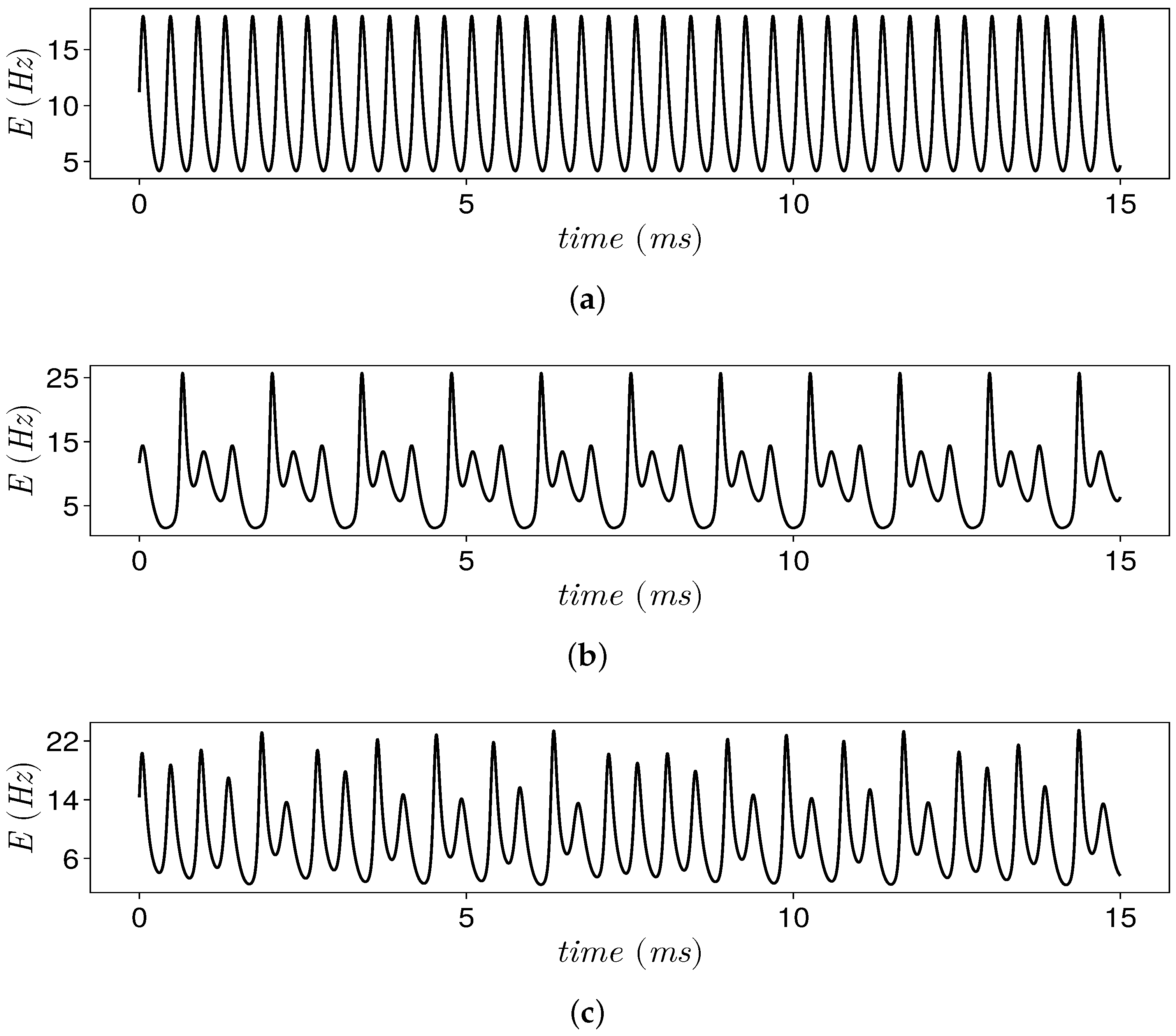
4.1. Patterns of Population Activity

To study and classify the patterns of population activity that can be reproduced by the model (5), a map of population activity was calculated on the plane of control parameters ( I 0 , U 0 ): I 0 [ 1.40 ; 1.709 ] , U 0 [ 0.30 ; 0.47 ] . (Figure 1a). Here, the red marker corresponds to the regions of chaotic activity, the blue marker corresponds to the regions of regular spiking activity, and the green marker corresponds to the regions of bursting activity. This map is accompanied by the map of the Lyapunov spectrum (Figure 1b).
The proposed reduced model, depending on the values of the control parameters I 0 and U 0 , can demonstrate a rich set of patterns of population activity, including regular spiking activity (Figure 2a) and bursting activity (Figure 2b), as well as chaotic activity (Figure 2c).
In the system (5), regions of multistability [60] were found, where several attractors coexist simultaneously in the phase space. For fixed U 0 = 0.3 , multistability can be observed, e.g., for I 0 [ 1.62 ; 1.59 ]. Depending on the chosen initial conditions, the phase point will be attracted to one of them, which, in turn, determines the pattern of population activity that will be observed. Figure 3 shows an example of coexistence of two attractors in the phase space of the system (5): a stable limit cycle (blue marker) and a strange chaotic attractor (red marker). This stable limit cycle is a mathematical image of regular bursting population activity, while the chaotic attractor is a mathematical image of a chaotic population activity. The chaotic regime was confirmed by calculating the spectrum of Lyapunov exponents. Note that multistability is a general property of such types of models and can be observed both in the original full model [36] and in the reduced model proposed in the present study.

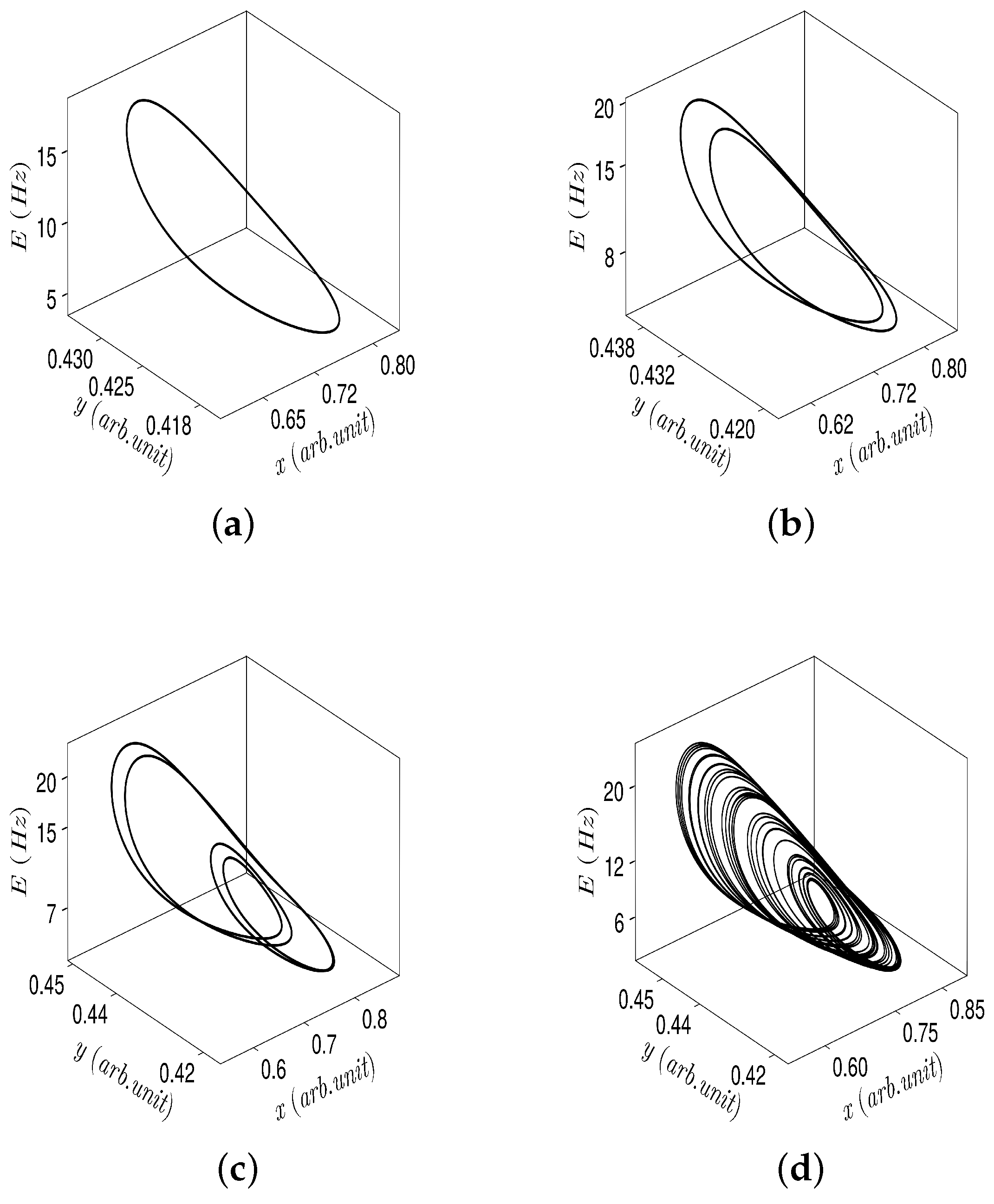
4.2. Bifurcation Analysis

Figure 4 presents a detailed one-parameter bifurcation analysis of the appearance of chaotic population activity in the system under consideration. Let us describe the main bifurcations that occur when the control parameter I 0 changes. The value of the second control parameter is fixed.
As can be seen from Figure 4 and Figure 5, when the value of parameter I 0 decreases, the limit cycle (corresponding to regular spiking activity), that was born earlier as a result of the Andronov–Hopf bifurcation from a stable equilibrium, undergoes a cascade of period-doubling bifurcations when the control parameter I 0 reaches the threshold value I 0 −1.497, see Figure 6. The multi-pass limit cycles that appear as a result of doubling bifurcations are mathematical images of regular bursting activity. When the threshold value I 0 −1.497 is reached, a strange attractor appears in the phase space of the system (5).
With a further decrease in the value of I 0 , the strange attractor is destroyed after which the trajectories go into a stable limit cycle, which appeared earlier in the vicinity of the chaotic attractor as a result of the Andronov–Hopf bifurcation.

4.3. Discussion

Note that the appearance of bursting and chaotic activity does not depend on the complexity of the local dynamics of neurons and glial cells and is determined only by the presence of a feedback loop between the presynaptic neuron and the glial cell. The demonstrated effects of neuron-like dynamics and neuron–glial interaction are quite general, as they do not imply specific characteristics of neuron–glial interaction, neural network architecture, or the dynamics of individual neurons. It should be noted that in the proposed model, we consider only the enhancement (potentiation) of synaptic transmission by astrocytes. The development of these studies can be considered within the framework of a simplified model of rhythmogenesis of bidirectional astrocytic regulation of neuronal activity [61].
Comparing our findings to the dynamics of the original full model [36], we observed the same types of patterns of population activity (spiking activity, bursting activity and chaotic activity). Nevertheless, the bifurcation mechanisms of transition to chaos differ. This fact highlights the connection between different types of synaptic potentiation and a particular way of transition to synchronous population patterns.

5. Conclusions

In this study, a new reduced mean-field model of neuron–glial interaction is proposed, which makes it possible to reproduce various types of population activity, such as spiking, bursting and chaotic synchronous patterns. The novelty of this study lies in the method of reducing the previously proposed model of bursting activity based on the classical Tsodyks–Markram model. The proposed model allows us to take into account the influence of glial cells on the dynamics of the system without consideration of the synaptic depression. Using two-parameter analysis, regions in the parameter space corresponding to the main types of population activity were identified. It was shown that for a certain range of values of governing parameters, patterns of regular and chaotic activity can coexist. The bifurcation mechanisms that lead to transition from one type of activity to another were investigated in detail.
The proposed mean-field model can be used to reproduce various patterns of population activity of neurons in a wide range of studies of dynamic memory and information processing. One of the possible applications of such research is the development of new effective methods for the treatment of neurological diseases associated with neuron–glial interaction.

Author Contributions

Conceptualization, S.V.S. and T.A.L.; methodology, S.V.S. and T.A.L.; software, S.M.O.; validation, S.V.S. and T.A.L.; formal analysis, S.M.O.; investigation, S.V.S., T.A.L. and S.M.O.; data curation, S.V.S., T.A.L. and S.M.O.; writing—original draft preparation, S.V.S., T.A.L. and S.M.O.; writing—review and editing, S.V.S., T.A.L. and S.M.O.; visualization, S.M.O.; supervision, S.V.S. and T.A.L.; project administration, S.V.S. and T.A.L.; funding acquisition, T.A.L. All authors have read and agreed to the published version of the manuscript.

Funding

This work was supported by the Russian Science Foundation (Project No. 19-72-10128).

Data Availability Statement

The data sets generated and/or analyzed during the current study are available from the corresponding author on reasonable request.

Acknowledgments

We are grateful to H.G.E. Meijer, C. Rackauckas and G. Datseris for their help with numerical calculations.

Conflicts of Interest

The authors declare no conflict of interest.

References

  1. Varela, F.; Lachaux, J.; Rodriguez, E.; Martinerie, J. The brainweb: Phase synchronization and large-scale integration. Nat. Rev. Neurosci. 2001, 2, 229–239. [Google Scholar] [CrossRef]
  2. Uhlhaas, P.; Singer, W. Neural synchrony in brain disorders: Relevance for cognitive dysfunctions and pathophysiology. Neuron 2006, 52, 155–168. [Google Scholar] [CrossRef] [PubMed]
  3. Lisman, J. Bursts as a unit of neural information: Making unreliable synapses reliable. Trends Neurosci. 1997, 20, 38–43. [Google Scholar] [CrossRef] [PubMed]
  4. Izhikevich, E.; Desai, N.; Walcott, E.; Hoppensteadt, F. Bursts as a unit of neural information: Selective communication via resonance. Trends Neurosci. 2003, 26, 161–167. [Google Scholar] [CrossRef] [PubMed]
  5. Gabbiani, F.; Metzner, W.; Wessel, R.; Koch, C. From stimulus encoding to feature extraction in weakly electric fish. Nature 1996, 384, 564–567. [Google Scholar] [CrossRef]
  6. Oswald, A.; Chacron, M.; Doiron, B.; Bastian, J.; Maler, L. Parallel processing of sensory input by bursts and isolated spikes. J. Neurosci. 2004, 24, 4351–4362. [Google Scholar] [CrossRef]
  7. Lesica, N.; Stanley, G. Encoding of natural scene movies by tonic and burst spikes in the lateral geniculate nucleus. J. Neurosci. 2004, 24, 10731–10740. [Google Scholar] [CrossRef]
  8. Reinagel, P.; Godwin, D.; Sherman, S.; Koch, C. Encoding of visual information by LGN bursts. J. Neurophysiol. 1999, 81, 2558–2569. [Google Scholar] [CrossRef]
  9. Segev, R.; Baruchi, I.; Hulata, E.; Ben-Jacob, E. Hidden neuronal correlations in cultured networks. Phys. Rev. Lett. 2004, 92, 118102. [Google Scholar] [CrossRef]
  10. Hulata, E.; Baruchi, I.; Segev, R.; Shapira, Y.; Ben-Jacob, E. Self-regulated complexity in cultured neuronal networks. Phys. Rev. Lett. 2004, 92, 198105. [Google Scholar] [CrossRef]
  11. Avoli, M.; Olivier, A. Bursting in human epileptogenic neocortex is depressed by an N-methyl-D-aspartate antagonist. Neurosci. Lett. 1987, 76, 249–254. [Google Scholar] [CrossRef] [PubMed]
  12. Hofer, K.T.; Kandracs, Á.; Tóth, K.; Hajnal, B.; Bokodi, V.; Toth, E.Z.; Erőss, L.; Entz, L.; Bago, A.G.; Fabo, D.; et al. Bursting of excitatory cells is linked to interictal epileptic discharge generation in humans. Sci. Rep. 2022, 12, 6280. [Google Scholar] [CrossRef]
  13. Ioannou, P.; Foster, D.L.; Sander, J.W.; Dupont, S.; Gil-Nagel, A.; Dragon O’Flaherty, E.; Alvarez-Baron, E.; Medjedovic, J. The burden of epilepsy and unmet need in people with focal seizures. Brain Behav. 2022, 12, e2589. [Google Scholar] [CrossRef] [PubMed]
  14. Lehnertz, K. Epilepsy: Extreme Events in the Human Brain. In Extreme Events in Nature and Society; Albeverio, S., Jentsch, V., Kantz, H., Eds.; The Frontiers Collection; Springer: Berlin/Heidelberg, Germany, 2006; pp. 123–143. ISBN 978-3-540-28610-3. [Google Scholar]
  15. Dingledine, R.; Varvel, N.H.; Dudek, F.E. When and How Do Seizures Kill Neurons, and Is Cell Death Relevant to Epileptogenesis? Adv. Exp. Med. Biol. 2014, 813, 109–122. [Google Scholar] [CrossRef] [PubMed]
  16. Devinsky, O.; Vezzani, A.; Najjar, S.; De Lanerolle, N.C.; Rogawski, M.A. Glia and epilepsy: Excitability and inflammation. Trends Neurosci. 2013, 36, 174–184. [Google Scholar] [CrossRef] [PubMed]
  17. Kim, S.Y.; Porter, B.E.; Friedman, A.; Kaufer, D. A potential role for glia-derived extracellular matrix remodeling in postinjury epilepsy. J. Neurosci. Res. 2016, 94, 794–803. [Google Scholar] [CrossRef] [PubMed]
  18. Patel, D.C.; Tewari, B.P.; Chaunsali, L.; Sontheimer, H. Neuron–glia interactions in the pathophysiology of epilepsy. Nat. Rev. Neurosci. 2019, 20, 282–297. [Google Scholar] [CrossRef] [PubMed]
  19. Shen, W.; Pristov, J.B.; Nobili, P.; Nikolić, L. Can glial cells save neurons in epilepsy? Neural Regen. Res. 2022, 18, 1417–1422. [Google Scholar] [CrossRef]
  20. Tian, G.; Azmi, H.; Takano, T.; Xu, Q.; Peng, W.; Lin, J.; Oberheim, N.; Lou, N.; Wang, X.; Zielke, H. An astrocytic basis of epilepsy. Nat. Med. 2005, 11, 973–981. [Google Scholar] [CrossRef]
  21. Seifert, G.; Steinhäuser, C. Neuron–astrocyte signaling and epilepsy. Exp. Neurol. 2013, 244, 4–10. [Google Scholar] [CrossRef]
  22. Henning, L.; Unichenko, P.; Bedner, P.; Steinhauser, C.; Henneberger, C. Overview article astrocytes as initiators of epilepsy. Neurochem. Res. 2023, 48, 1091–1099. [Google Scholar] [CrossRef] [PubMed]
  23. Crunfli, F.; Carregari, V.C.; Veras, F.P.; Silva, L.S.; Nogueira, M.H.; Antunes, A.S.L.M.; Vendramini, P.H.; Valença, A.G.F.; Brandão-Teles, C.; da Silva Zuccoli, G.; et al. Morphological, cellular, and molecular basis of brain infection in COVID-19 patients. Proc. Natl. Acad. Sci. USA 2022, 119, e2200960119. [Google Scholar] [CrossRef] [PubMed]
  24. Hanson, B.A.; Visvabharathy, L.; Ali, S.T.; Kang, A.K.; Patel, T.R.; Clark, J.R.; Lim, P.H.; Orban, Z.S.; Hwang, S.S.; Mattoon, D.; et al. Plasma Biomarkers of Neuropathogenesis in Hospitalized Patients with COVID-19 and Those with Postacute Sequelae of SARS-CoV-2 Infection. Neurol.-Neuroimmunol. Neuroinflamm. 2022, 9, 1–11. [Google Scholar] [CrossRef] [PubMed]
  25. Stasenko, S.; Hramov, A.; Kazantsev, V. Loss of neuron network coherence induced by virus-infected astrocytes: A model study. Sci. Rep. 2023, 13, 6401. [Google Scholar] [CrossRef] [PubMed]
  26. Sibille, J.; Zapata, J.; Teillon, J.; Rouach, N. Astroglial calcium signaling displays short-term plasticity and adjusts synaptic efficacy. Front. Cell. Neurosci. 2015, 189. [Google Scholar] [CrossRef]
  27. Haydon, P.G.; Nedergaard, M. How do astrocytes participate in neural plasticity? Cold Spring Harb. Perspect. Biol. 2015, 7, a020438. [Google Scholar] [CrossRef]
  28. Halassa, M.M.; Haydon, P.G. Integrated brain circuits: Astrocytic networks modulate neuronal activity and behavior. Annu. Rev. Physiol. 2010, 72, 335–355. [Google Scholar] [CrossRef]
  29. Jolivet, R.; Coggan, J.S.; Allaman, I.; Magistretti, P.J. Multi-timescale modeling of activity-dependent metabolic coupling in the neuron-glia-vasculature ensemble. PLoS Comput. Biol. 2015, 11, e1004036. [Google Scholar] [CrossRef]
  30. Linne, M.L.; Aćimović, J.; Saudargiene, A.; Manninen, T. Neuron–Glia Interactions and Brain Circuits. In Computational Modelling of the Brain: Modelling Approaches to Cells, Circuits and Networks; Springer International Publishing: Cham, Switzerland, 2022; pp. 87–103. [Google Scholar] [CrossRef]
  31. Araque, A.; Parpura, V.; Sanzgiri, R.P.; Haydon, P.G. Glutamate-dependent astrocyte modulation of synaptic transmission between cultured hippocampal neurons. Eur. J. Neurosci. 1998, 10, 2129–2142. [Google Scholar] [CrossRef]
  32. Araque, A.; Parpura, V.; Sanzgiri, R.P.; Haydon, P.G. Tripartite synapses: Glia, the unacknowledged partner. Trends Neurosci. 1999, 22, 208–215. [Google Scholar] [CrossRef]
  33. Markram, H.; Tsodyks, M. Redistribution of synaptic efficacy between neocortical pyramidal neurons. Nature 1996, 382, 807–810. [Google Scholar] [CrossRef]
  34. Masquelier, T.; Deco, G. Network bursting dynamics in excitatory cortical neuron cultures results from the combination of different adaptive mechanism. PLoS ONE 2013, 8, e75824. [Google Scholar] [CrossRef]
  35. Barabash, N.; Levanova, T.; Stasenko, S. STSP model with neuron-glial interaction produced bursting activity. In Proceedings of the 2021 Third International Conference Neurotechnologies and Neurointerfaces (CNN), Kaliningrad, Russia, 13–15 September 2021; pp. 12–15. [Google Scholar] [CrossRef]
  36. Barabash, N.; Levanova, T.; Stasenko, S. Rhythmogenesis in the mean field model of the neuron–glial network. Eur. Phys. J. Spec. Top. 2023, 1–6. [Google Scholar] [CrossRef]
  37. Stasenko, S.V.; Lazarevich, I.A.; Kazantsev, V.B. Quasi-synchronous neuronal activity of the network induced by astrocytes. Procedia Comput. Sci. 2020, 169, 704–709. [Google Scholar] [CrossRef]
  38. Pankratova, E.V.; Kalyakulina, A.I.; Stasenko, S.V.; Gordleeva, S.Y.; Lazarevich, I.A.; Kazantsev, V.B. Neuronal synchronization enhanced by neuron–astrocyte interaction. Nonlinear Dyn. 2019, 97, 647–662. [Google Scholar] [CrossRef]
  39. Lazarevich, I.A.; Stasenko, S.V.; Kazantsev, V.B. Synaptic multistability and network synchronization induced by the neuron–glial interaction in the brain. JETP Lett. 2017, 105, 210–213. [Google Scholar] [CrossRef]
  40. Stasenko, S.V.; Kazantsev, V.B. Dynamic Image Representation in a Spiking Neural Network Supplied by Astrocytes. Mathematics 2023, 11, 561. [Google Scholar] [CrossRef]
  41. Gordleeva, S.Y.; Tsybina, Y.A.; Krivonosov, M.I.; Ivanchenko, M.V.; Zaikin, A.A.; Kazantsev, V.B.; Gorban, A.N. Modeling working memory in a spiking neuron network accompanied by astrocytes. Front. Cell. Neurosci. 2021, 15, 631485. [Google Scholar] [CrossRef]
  42. Tsybina, Y.; Kastalskiy, I.; Krivonosov, M.; Zaikin, A.; Kazantsev, V.; Gorban, A.N.; Gordleeva, S. Astrocytes mediate analogous memory in a multi-layer neuron–astrocyte network Neural. Comput. Appl. 2022, 34, 9147–9160. [Google Scholar] [CrossRef]
  43. Volman, V.; Bazhenov, M.; Sejnowski, T.J. Computational models of neuron-astrocyte interaction in epilepsy. Front. Comput. Neurosci. 2012, 6, 58. [Google Scholar] [CrossRef]
  44. Eid, T. Transforming Glia to Neurons Effectively Treats Temporal Lobe Seizures. Epilepsy Curr. 2022, 22, 130–131. [Google Scholar] [CrossRef]
  45. Mongillo, G.; Barak, O.; Tsodyks, M. Synaptic theory of working memory. Science 2008, 319, 1543–1546. [Google Scholar] [CrossRef]
  46. Wilson, H.R.; Cowan, J.D. Excitatory and inhibitory interactions in localized populations of model neurons. Biophys. J. 1972, 12, 1–24. [Google Scholar] [CrossRef]
  47. Tsodyks, M.; Pawelzik, K.; Markram, H. Neural networks with dynamic synapses. Neural Comput. 1998, 10, 821–835. [Google Scholar] [CrossRef] [PubMed]
  48. Perea, G.; Navarrete, M.; Araque, A. Tripartite synapses: Astrocytes process and control synaptic information. Trends Neurosci. 2009, 32, 421–431. [Google Scholar] [CrossRef]
  49. Agulhon, C.; Petravicz, J.; McMullen, A.; Sweger, E.; Minton, S.; Taves, S.; Casper, K.; Fiacco, T.; McCarthy, K. What is the role of astrocyte calcium in neurophysiology? Neuron 2008, 59, 932–946. [Google Scholar] [CrossRef] [PubMed]
  50. Barres, B. The mystery and magic of glia: A perspective on their roles in health and disease. Neuron 2008, 60, 430–440. [Google Scholar] [CrossRef] [PubMed]
  51. Benettin, G.; Galgani, L.; Giorgilli, A.; Strelcyn, J.M. Lyapunov characteristic exponents for smooth dynamical systems and for Hamiltonian systems; a method for computing all of them. Part 1: Theory. Meccanica 1980, 15, 9–20. [Google Scholar] [CrossRef]
  52. Borisov, A.V.; Jalnine, A.Y.; Kuznetsov, S.P.; Sataev, I.R.; Sedova, J.V. Dynamical phenomena occurring due to phase volume compression in nonholonomic model of the rattleback. Regul. Chaotic Dyn. 2012, 17, 512–532. [Google Scholar] [CrossRef]
  53. Borisov, A.V.; Kazakov, A.O.; Sataev, I.R. The reversal and chaotic attractor in the nonholonomic model of Chaplygin’s top. Regul. Chaotic Dyn. 2014, 19, 718–733. [Google Scholar] [CrossRef]
  54. Kazakov, A. On bifurcations of Lorenz attractors in the Lyubimov–Zaks model. Chaos Interdiscip. J. Nonlinear Sci. 2021, 31, 093118. [Google Scholar] [CrossRef] [PubMed]
  55. Karatetskaia, E.; Shykhmamedov, A.; Kazakov, A. Shilnikov attractors in three-dimensional orientation-reversing maps. Chaos Interdiscip. J. Nonlinear Sci. 2021, 31, 011102. [Google Scholar] [CrossRef] [PubMed]
  56. Levanova, T.A.; Kazakov, A.O.; Osipov, G.V.; Kurths, J. Dynamics of ensemble of inhibitory coupled Rulkov maps. Eur. Phys. J. Spec. Top. 2016, 225, 147–157. [Google Scholar] [CrossRef]
  57. Datseris, G.; Wagemakers, A. Effortless estimation of basins of attraction. Chaos Interdiscip. J. Nonlinear Sci. 2022, 32, 023104. [Google Scholar] [CrossRef] [PubMed]
  58. Datseris, G. DynamicalSystems. jl: A Julia software library for chaos and nonlinear dynamics. J. Open Source Softw. 2018, 3, 598. [Google Scholar] [CrossRef]
  59. Datseris, G.; Parlitz, U. Nonlinear Dynamics: A Concise Introduction Interlaced with Code; Springer Nature: Berlin/Heidelberg, Germany, 2022. [Google Scholar]
  60. Pisarchik, A.N.; Hramov, A.E. Multistability in Physical and Living Systems; Springer: Berlin/Heidelberg, Germany, 2022; Volume 2, pp. 1–408. [Google Scholar] [CrossRef]
  61. Gordleeva, S.Y.; Stasenko, S.V.; Semyanov, A.V.; Dityatev, A.E.; Kazantsev, V.B. Bi-directional astrocytic regulation of neuronal activity within a network. Front. Comput. Neurosci. 2012, 6, 92. [Google Scholar] [CrossRef]
Figure 1. (a) Map of population activity patterns on the parameter plane ( I 0 , U 0 ), I 0 [−1.40; −1.709], U 0 [ 0.30 ; 0.47 ] . The red marker corresponds to regions of chaotic activity, the blue marker corresponds to regions of regular spiking activity, and the green marker corresponds to regions of regular bursting activity. (b) Map of Lyapunov spectrum. The green marker corresponds to the (0, −, −) spectrum, the light blue marker corresponds to the (0, 0, −) spectrum, and the red marker corresponds to the (+, 0, −) spectrum.
Mathematics 11 02143 g001
Figure 2. Time series for variable E ( t ) . (a) Regular spiking activity, I 0 = −1.4. (b) Regular bursting activity, I 0 = −1.65. (c) Chaotic activity, I 0 = 1.59 . The value of the parameter that sets the probability of neurotransmitter release is fixed, U 0 = 0.3 .
Mathematics 11 02143 g002
Figure 3. (a) A stable limit cycle (blue marker) and a chaotic attractor (red marker) coexisting in the phase space of the system (5). (b) Time series. Regular (blue marker) and chaotic (red marker) population activity. Control parameter values: I 0 = −1.6, U 0 = 0.3 .
Mathematics 11 02143 g003
Figure 4. Bifurcation diagram and Lyapunov spectrum, I 0 [−1.4; −1.709], U 0 = 0.3 .
Mathematics 11 02143 g004
Figure 5. Bifurcation diagram and Lyapunov spectrum, I 0 [−1.4; −1.709], U 0 = 0.35 .
Mathematics 11 02143 g005
Figure 6. Phase portraits of the system (5) for different values of I 0 : (a) I 0 = −1.4—limit cycle, (b) I 0 = −1.49854042—two-period limit cycle, (c) I 0 = −1.56203902—four-period limit cycle, and (d) I 0 = −1.59—chaotic attractor. In all cases U 0 = 0.3 .
Mathematics 11 02143 g006
Disclaimer/Publisher’s Note: The statements, opinions and data contained in all publications are solely those of the individual author(s) and contributor(s) and not of MDPI and/or the editor(s). MDPI and/or the editor(s) disclaim responsibility for any injury to people or property resulting from any ideas, methods, instructions or products referred to in the content.

