A NumericalInvestigation for a Class of Transient-State Variable Coefficient DCR Equations

Abstract

In this paper, a combined Laplace transform (LT) and boundary element method (BEM) is used to find numerical solutions to problems of anisotropic functionally graded media that are governed by the transient diffusion–convection–reaction equation. First, the variable coefficient governing equation is reduced to a constant coefficient equation. Then, the Laplace-transformed constant coefficients equation is transformed into a boundary-only integral equation. Using a BEM, the numerical solutions in the frame of the Laplace transform may then be obtained from this integral equation. Then, the solutions are inversely transformed numerically back to the original time variable using the Stehfest formula. The numerical solutions are verified by showing their accuracy and steady state. For symmetric problems, the symmetry of solutions is also justified. Moreover, the effects of the anisotropy and inhomogeneity of the material on the solutions are also shown, to suggest that it is important to take the anisotropy and inhomogeneity into account when performing experimental studies.

1. Introduction

Insights on flow in porous media may be obtained from [1,2,3,4]. Over the last ten years, functionally graded materials (FGMs) have become a popular research topic, and many studies have been conducted on FGMs for various applications. FGMs are defined by authors as materials that are inhomogeneous and have properties such as thermal conductivity, hardness, toughness, ductility, and corrosion resistance, which change spatially in a continuous manner. Commonly, the properties of the considered material for a specific application are represented by the coefficients of the governing equation. In this case, the coefficients should be constant if—and only if—the material is homogeneous.

The diffusion convection reaction (DCR) equation is usually used as the governing equation for many applications in engineering, medicine, biology, and ecology. Several studies have been conducted to find numerical solutions to the DCR equation. These studies include Fendoğlu et al. [5] in 2018, Wang and Ang [6] in 2018, Sheu et al. [7] in 2000, Xu [8] in 2018, and AL-Bayati and Wrobel [9] in 2019, who considered the DCR equation with constant coefficients. Samec and Škerget [10] in 2004, Rocca et al. [11] in 2005, and AL-Bayati and Wrobel [12,13] in 2018 studied the DCR equation with variable velocity. Martinez et al. [14] in 2013 used nonstandard finite difference schemes based on Green’s function formulations for reaction–diffusion–convection systems. Only a limited number of studies on the steady-state equation of variable coefficients have been performed (see, for example, [15]).

This paper is aimed at studying problems that are governed by a DCR equation with variable coefficients. Specifically, this paper will extend the recently published work of [15] on the steady-state DCR equation to the unsteady-state DCR equation of variable coefficients (for anisotropic functionally graded materials) of the form

$$\frac{\partial }{\partial x_i}\left[d_{ij}\left(\mathbf{x}\right)\frac{\partial c\left(\mathbf{x},t\right)}{\partial x_j}\right]-\frac{\partial }{\partial x_i}\left[v_i\left(\mathbf{x}\right)c\left(\mathbf{x},t\right)\right]-k\left(\mathbf{x}\right)c\left(\mathbf{x},t\right)=\alpha \left(\mathbf{x},t\right)\frac{\partial c\left(\mathbf{x},t\right)}{\partial t}$$

(1)

The continuously varying coefficients $d_{ij},v_i,k,\alpha$ in (1) represent the anisotropic diffusivity, velocity, decay reaction, and change rate coefficients of the medium of interest, respectively. Therefore, Equation (1) is relevant for FGMs. Equation (1) covers a wider class of problems since it applies to anisotropic and inhomogeneous media, nonetheless including the case of isotropic diffusion taking place when $d_{11}=d_{22},d_{12}=0$ as well as the case of homogeneous media that appear when the coefficients $d_{ij}\left(\mathbf{x}\right)$, $v_i\left(\mathbf{x}\right)$, $k\left(\mathbf{x}\right)$ and $\alpha \left(\mathbf{x},t\right)$ are constant.

2. The Governing Equation, Initial and Boundary Conditions

Referring to the Cartesian frame $O{x}_1{x}_2$, we will discuss the initial boundary value problems governed by (1) where $\mathbf{x}=\left(x_1,x_2\right)$. The coefficient $\left[d_{ij}\right]$$\left(i,j=1,2\right)$ is a real positive definite symmetrical matrix. Moreover, in (1), the summation convention for repeated indices applies, so (1) can explicitly be written as

$$\begin{array}{ccc}& & \frac{\partial }{\partial x_1}\left(d_{11}\frac{\partial c}{\partial x_1}\right)+\frac{\partial }{\partial x_1}\left(d_{12}\frac{\partial c}{\partial x_2}\right)+\frac{\partial }{\partial x_2}\left(d_{12}\frac{\partial c}{\partial x_1}\right)+\frac{\partial }{\partial x_2}\left(d_{22}\frac{\partial c}{\partial x_2}\right)\hfill \\ & & -\frac{\partial }{\partial x_1}\left(v_{1}c\right)-\frac{\partial }{\partial x_2}\left(v_{2}c\right)-kc=\alpha \frac{\partial c}{\partial t}\hfill \end{array}$$

(2)

By knowing the coefficients of $d_{ij}\left(\mathbf{x}\right),v_i\left(\mathbf{x}\right),k\left(\mathbf{x}\right),\alpha \left(\mathbf{x},t\right)$, solutions $c\left(\mathbf{x},t\right)$ to (1) and its derivatives will be sought within the time interval $t\ge 0$ and region $\mathsf{\Omega }$ in $R^2$, with boundary $\partial \mathsf{\Omega }$ consisting of a finite number of piecewise smooth curves. On $\partial {\mathsf{\Omega }}_1$, the dependent variable $c\left(\mathbf{x},t\right)$ is specified, and

$$F\left(\mathbf{x},t\right)=d_{ij}\left(\mathbf{x}\right)\frac{\partial c\left(\mathbf{x},t\right)}{\partial x_i}{n}_j$$

(3)

is specified on $\partial {\mathsf{\Omega }}_2$, where $\partial \mathsf{\Omega }=\partial {\mathsf{\Omega }}_1\cup \partial {\mathsf{\Omega }}_2$ and $\mathbf{n}=\left(n_1,n_2\right)$ represents the outward pointing normal to $\partial \mathsf{\Omega }$. The initial condition is

$$c\left(\mathbf{x},0\right)=0$$

(4)

3. Derivation of an Integral Equation

We restrict the coefficients $d_{ij},v_i,k,\alpha$ to be of the form

$$\begin{array}{ccc}\hfill d_{ij}\left(\mathbf{x}\right)& =& {\widehat{d}}_{ij}h\left(\mathbf{x}\right)\hfill \end{array}$$

(5)

$$\begin{array}{ccc}\hfill v_i\left(\mathbf{x}\right)& =& {\widehat{v}}_{i}h\left(\mathbf{x}\right)\hfill \end{array}$$

(6)

$$\begin{array}{ccc}\hfill k\left(\mathbf{x}\right)& =& \widehat{k}h\left(\mathbf{x}\right)\hfill \end{array}$$

(7)

$$\begin{array}{ccc}\hfill \alpha \left(\mathbf{x},t\right)& =& \widehat{\alpha }\left(t\right)h\left(\mathbf{x}\right)\hfill \end{array}$$

(8)

where $h\left(\mathbf{x}\right)$ is a differentiable function; ${\widehat{d}}_{ij},{\widehat{v}}_i,\widehat{k}$ are constants; and $\widehat{\alpha }\left(t\right)$ is a function of time t. The substitution of (5)–(8) into (1) gives

$${\widehat{d}}_{ij}\frac{\partial }{\partial x_i}\left(h\frac{\partial c}{\partial x_j}\right)-{\widehat{v}}_i\frac{\partial \left(hc\right)}{\partial x_i}-\widehat{k}hc=\widehat{\alpha }h\frac{\partial c}{\partial t}$$

(9)

Assume

$$c\left(\mathbf{x},t\right)=h^{-1/2}\left(\mathbf{x}\right)\psi \left(\mathbf{x},t\right)$$

(10)

Therefore, using (5) and (10) in (3) gives

$$F\left(\mathbf{x},t\right)=-F_h\left(\mathbf{x}\right)\psi \left(\mathbf{x},t\right)+h^{1/2}\left(\mathbf{x}\right)F_{\psi }\left(\mathbf{x},t\right)$$

(11)

where

$$F_h\left(\mathbf{x}\right)={\widehat{d}}_{ij}\frac{\partial h^{1/2}\left(\mathbf{x}\right)}{\partial x_j}{n}_i{F}_{\psi }\left(\mathbf{x},t\right)={\widehat{d}}_{ij}\frac{\partial \psi \left(\mathbf{x},t\right)}{\partial x_j}{n}_i$$

(12)

Moreover, Equation (9) can be written as

$${\widehat{d}}_{ij}\frac{\partial }{\partial x_i}\left[h\frac{\partial \left(h^{-1/2}\psi \right)}{\partial x_j}\right]-{\widehat{v}}_i\frac{\partial \left(h^{1/2}\psi \right)}{\partial x_i}-\widehat{k}{h}^{1/2}\psi =\widehat{\alpha }h\frac{\partial \left(h^{-1/2}\psi \right)}{\partial t}$$

(13)

That is,

$${\widehat{d}}_{ij}\frac{\partial }{\partial x_i}\left[h\left(h^{-1/2}\frac{\partial \psi }{\partial x_j}+\psi \frac{\partial h^{-1/2}}{\partial x_j}\right)\right]-{\widehat{v}}_i\left(h^{1/2}\frac{\partial \psi }{\partial x_i}+\psi \frac{\partial h^{1/2}}{\partial x_i}\right)-\widehat{k}{h}^{1/2}\psi =\widehat{\alpha }h\left(h^{-1/2}\frac{\partial \psi }{\partial t}\right)$$

(14)

or

$${\widehat{d}}_{ij}\frac{\partial }{\partial x_i}\left(h^{1/2}\frac{\partial \psi }{\partial x_j}+h\psi \frac{\partial h^{-1/2}}{\partial x_j}\right)-{\widehat{v}}_i\left(h^{1/2}\frac{\partial \psi }{\partial x_i}+\psi \frac{\partial h^{1/2}}{\partial x_i}\right)-\widehat{k}{h}^{1/2}\psi =\widehat{\alpha }{h}^{1/2}\frac{\partial \psi }{\partial t}$$

(15)

Using the identity

$$\frac{\partial h^{-1/2}}{\partial x_i}=-h^{-1}\frac{\partial h^{1/2}}{\partial x_i}$$

(16)

implies

$${\widehat{d}}_{ij}\frac{\partial }{\partial x_i}\left(h^{1/2}\frac{\partial \psi }{\partial x_j}-\psi \frac{\partial h^{1/2}}{\partial x_j}\right)-{\widehat{v}}_i\left(h^{1/2}\frac{\partial \psi }{\partial x_i}+\psi \frac{\partial h^{1/2}}{\partial x_i}\right)-\widehat{k}{h}^{1/2}\psi =\widehat{\alpha }{h}^{1/2}\frac{\partial \psi }{\partial t}$$

(17)

Rearranging and neglecting some zero terms gives

$$h^{1/2}\left({\widehat{d}}_{ij}\frac{{\partial }^2\psi }{\partial x_i\partial x_j}-{\widehat{v}}_i\frac{\partial \psi }{\partial x_i}\right)-\psi \left({\widehat{d}}_{ij}\frac{{\partial }^2{h}^{1/2}}{\partial x_i\partial x_j}+{\widehat{v}}_i\frac{\partial h^{1/2}}{\partial x_i}\right)-\widehat{k}{h}^{1/2}\psi =\widehat{\alpha }{h}^{1/2}\frac{\partial \psi }{\partial t}$$

(18)

so that if h satisfies

$${\widehat{d}}_{ij}\frac{{\partial }^2{h}^{1/2}}{\partial x_i\partial x_j}+{\widehat{v}}_i\frac{\partial h^{1/2}}{\partial x_i}-\lambda h^{1/2}=0$$

(19)

where $\lambda$ is a constant, then the transformation (10) takes the variable coefficient Equation (1) into a constant coefficient equation:

$${\widehat{d}}_{ij}\frac{{\partial }^2\psi }{\partial x_i\partial x_j}-{\widehat{v}}_i\frac{\partial \psi }{\partial x_i}-\left(\lambda +\widehat{k}\right)\psi =\widehat{\alpha }\frac{\partial \psi }{\partial t}$$

(20)

Taking the Laplace transform of (10), (11), (20) and applying the initial condition (4), we obtain

$${\psi }^{*}\left(\mathbf{x},s\right)=h^{1/2}\left(\mathbf{x}\right)c^{*}\left(\mathbf{x},s\right)$$

(21)

$$F_{{\psi }^{*}}\left(\mathbf{x},s\right)=\left[F^{*}\left(\mathbf{x},s\right)+F_h\left(\mathbf{x}\right){\psi }^{*}\left(\mathbf{x},s\right)\right]h^{-1/2}\left(\mathbf{x}\right)$$

(22)

$${\widehat{d}}_{ij}\frac{{\partial }^2{\psi }^{*}}{\partial x_i\partial x_j}-{\widehat{v}}_i\frac{\partial {\psi }^{*}}{\partial x_i}-\left(\lambda +\widehat{k}+s{\widehat{\alpha }}^{*}\right){\psi }^{*}=0$$

(23)

Using the Gauss divergence theorem, Equation (23) can be transformed into a boundary integral equation:

$$\begin{array}{ccc}\hfill \eta \left(\mathit{\zeta }\right){\psi }^{*}\left(\mathit{\zeta },s\right)& =& {\int }_{\partial \mathsf{\Omega }}\left\{F_{{\psi }^{*}}\left(\mathbf{x},s\right)\Phi \left(\mathbf{x},\mathit{\zeta }\right)-\left[F\left(\mathbf{x}\right)\Phi \left(\mathbf{x},\mathit{\zeta }\right)\right.\right.\hfill \\ & & \left.\left.+\Gamma \left(\mathbf{x},\mathit{\zeta }\right)\right]{\psi }^{*}\left(\mathbf{x},s\right)\right\}dS\left(\mathbf{x}\right)\hfill \end{array}$$

(24)

where $\eta =0$ if $\zeta \notin \mathsf{\Omega }$, $\eta =1/2$ if $\zeta \in \partial \mathsf{\Omega }$, $\eta =1$ if $\zeta \in \mathsf{\Omega }$, $F_v\left(\mathbf{x}\right)={\widehat{v}}_i{n}_i\left(\mathbf{x}\right)$. For 2D problems, the fundamental solutions $\Phi (\mathbf{x},\mathit{\zeta })$ and $\Gamma (\mathbf{x},\mathit{\zeta })$ are given as

$$\begin{array}{ccc}\hfill \Phi (\mathbf{x},\mathit{\zeta })& =& \frac{{\rho }_i}{2\pi D}exp\left(-\frac{\dot{\mathbf{v}}.\dot{\mathbf{R}}}{2D}\right)K_0\left(\mu \dot{R}\right)\hfill \end{array}$$

(25)

$$\begin{array}{ccc}\hfill \Gamma (\mathbf{x},\mathit{\zeta })& =& {\widehat{d}}_{ij}\frac{\partial \Phi \left(\mathbf{x},\mathit{\zeta }\right)}{\partial x_j}{n}_i\hfill \end{array}$$

(26)

where

$$\begin{array}{ccc}\hfill \mu & =& \sqrt{{\left(\dot{v}/2D\right)}^2+\left[\left(\lambda +\widehat{k}+s{\widehat{\alpha }}^{*}\right)/D\right]}\hfill \end{array}$$

(27)

$$\begin{array}{ccc}\hfill D& =& \left[{\widehat{d}}_{11}+2{\widehat{d}}_{12}{\rho }_r+{\widehat{d}}_{22}\left({\rho }_r^2+{\rho }_i^2\right)\right]/2\hfill \end{array}$$

(28)

$$\begin{array}{ccc}\hfill \dot{\mathbf{R}}& =& \dot{\mathbf{x}}-\dot{\mathit{\zeta }}\hfill \end{array}$$

(29)

$$\begin{array}{ccc}\hfill \dot{\mathbf{x}}& =& \left(x_1+{\rho }_r{x}_2,{\rho }_i{x}_2\right)\hfill \end{array}$$

(30)

$$\begin{array}{ccc}\hfill \dot{\mathit{\zeta }}& =& \left({\zeta }_1+{\rho }_r{\zeta }_2,{\rho }_i{\zeta }_2\right)\hfill \end{array}$$

(31)

$$\begin{array}{ccc}\hfill \dot{\mathbf{v}}& =& \left({\widehat{v}}_1+{\rho }_r{\widehat{v}}_2,{\rho }_i{\widehat{v}}_2\right)\hfill \end{array}$$

(32)

$$\begin{array}{ccc}\hfill \dot{R}& =& \sqrt{{\left(x_1+{\rho }_r{x}_2-{\zeta }_1-{\rho }_r{\zeta }_2\right)}^2+{\left({\rho }_i{x}_2-{\rho }_i{\zeta }_2\right)}^2}\hfill \end{array}$$

(33)

$$\begin{array}{ccc}\hfill \dot{v}& =& \sqrt{{\left({\widehat{v}}_1+{\rho }_r{\widehat{v}}_2\right)}^2+{\left({\rho }_i{\widehat{v}}_2\right)}^2}\hfill \end{array}$$

(34)

and ${\rho }_r$ and ${\rho }_i$ are the real and the positive imaginary parts of the complex root $\rho$ of the quadratic equation ${\widehat{d}}_{11}+2{\widehat{d}}_{12}\rho +{\widehat{d}}_{22}{\rho }^2=0$, respectively, and $K_0$ is the modified Bessel function. Using (21) and (22) in (24) yields

$$\eta h^{1/2}{c}^{*}={\int }_{\partial \mathsf{\Omega }}\left\{\left(h^{-1/2}\Phi \right)F^{*}+\left[\left(F_h-F_v{h}^{1/2}\right)\Phi -h^{1/2}\Gamma \right]c^{*}\right\}dS$$

(35)

Equation (35) provides a boundary integral equation for determining the numerical solutions of $c^{*}$ and its derivatives at all points of $\mathsf{\Omega }$. The derivative solutions $\partial c^{*}/\partial {\xi }_1$ and $\partial c^{*}/\partial {\xi }_2$ can be determined using the following equations:

$$\frac{\partial c^{*}}{\partial {\zeta }_1}=h^{-1/2}\left[{\int }_{\partial \mathsf{\Omega }}\left\{\left(h^{-1/2}\frac{\partial \Phi }{\partial {\zeta }_1}\right)F^{*}+\left[\left(F_h-F_v{h}^{1/2}\right)\frac{\partial \Phi }{\partial {\zeta }_1}-h^{1/2}\frac{\partial \Gamma }{\partial {\zeta }_1}\right]c^{*}\right\}dS-c^{*}\frac{\partial h^{1/2}}{\partial {\zeta }_1}\right]$$

(36)

$$\frac{\partial c^{*}}{\partial {\zeta }_2}=h^{-1/2}\left[{\int }_{\partial \mathsf{\Omega }}\left\{\left(h^{-1/2}\frac{\partial \Phi }{\partial {\zeta }_2}\right)F^{*}+\left[\left(F_h-F_v{h}^{1/2}\right)\frac{\partial \Phi }{\partial {\zeta }_2}-h^{1/2}\frac{\partial \Gamma }{\partial {\zeta }_2}\right]c^{*}\right\}dS-c^{*}\frac{\partial h^{1/2}}{\partial {\zeta }_2}\right]$$

(37)

Knowing the solutions of $c^{*}\left(\mathbf{x},s\right)$ and its derivatives $\partial c^{*}/\partial x_1$ and $\partial c^{*}/\partial x_2$ from (35), the numerical Laplace transform inversion technique using the Stehfest formula is then employed to find the values of $c\left(\mathbf{x},t\right)$ and its derivatives $\partial c/\partial x_1$ and $\partial c/\partial x_2$. The Stehfest formula is

$$\begin{array}{ccc}\hfill c\left(\mathbf{x},t\right)& \simeq & \frac{ln2}{t}\sum _{m=1}^N{V}_m{c}^{*}\left(\mathbf{x},s_m\right)\hfill \\ \hfill \frac{\partial c\left(\mathbf{x},t\right)}{\partial x_1}& \simeq & \frac{ln2}{t}\sum _{m=1}^N{V}_m\frac{\partial c^{*}\left(\mathbf{x},s_m\right)}{\partial x_1}\hfill \\ \hfill \frac{\partial c\left(\mathbf{x},t\right)}{\partial x_2}& \simeq & \frac{ln2}{t}\sum _{m=1}^N{V}_m\frac{\partial c^{*}\left(\mathbf{x},s_m\right)}{\partial x_2}\hfill \end{array}$$

(38)

where

$$\begin{array}{ccc}\hfill s_m& =& \frac{ln2}{t}m\hfill \end{array}$$

(39)

$$\begin{array}{ccc}\hfill V_m& =& {\left(-1\right)}^{\frac{N}{2}+m}\sum _{k=\left[\frac{m+1}{2}\right]}^{min\left(m,\frac{N}{2}\right)}\frac{k^{N/2}\left(2k\right)!}{\left(\frac{N}{2}-k\right)!k!\left(k-1\right)!\left(m-k\right)!\left(2k-m\right)!}\hfill \end{array}$$

(40)

Possible multiparameter solutions $h\left(\mathbf{x}\right)$ to (19) are

$$\begin{array}{ccc}\hfill h\left(\mathbf{x}\right)& =& \begin{array}{c}\left\{\begin{array}{c}\mathrm{constant},\lambda =0\hfill \\ {\left[exp\left({\beta }_0+{\beta }_i{x}_i\right)\right]}^2,{\widehat{d}}_{ij}{\beta }_i{\beta }_j+{\widehat{v}}_i{\beta }_i-\lambda =0\hfill \end{array}\right.\hfill \end{array}\hfill \end{array}$$

(41)

If the flow is incompressible, that is, the divergence of the velocity is zero, then

$$\frac{\partial v_i\left(\mathbf{x}\right)}{\partial x_i}=0$$

(42)

Therefore, the governing Equation (1) reduces to

$$\frac{\partial }{\partial x_i}\left[d_{ij}\left(\mathbf{x}\right)\frac{\partial c\left(\mathbf{x},t\right)}{\partial x_j}\right]-v_i\left(\mathbf{x}\right)\frac{\partial c\left(\mathbf{x},t\right)}{\partial x_i}-k\left(\mathbf{x}\right)c\left(\mathbf{x},t\right)=\alpha \left(\mathbf{x}\right)\frac{\partial c\left(\mathbf{x},t\right)}{\partial t}$$

(43)

Moreover, from (6), we obtain

$$\frac{\partial v_i\left(\mathbf{x}\right)}{\partial x_i}=2h^{1/2}\left(\mathbf{x}\right){\widehat{v}}_i\frac{\partial h^{1/2}\left(\mathbf{x}\right)}{\partial x_i}=0$$

(44)

so that

$${\widehat{v}}_i\frac{\partial h^{1/2}\left(\mathbf{x}\right)}{\partial x_i}=0$$

(45)

Therefore, Equation (19) reduces to

$${\widehat{d}}_{ij}\frac{{\partial }^2{h}^{1/2}}{\partial x_i\partial x_j}-\lambda h^{1/2}=0$$

(46)

Thus, for incompressible flow, possible multiparameter functions $h\left(\mathbf{x}\right)$ satisfying (46) are

$$\begin{array}{ccc}\hfill h\left(\mathbf{x}\right)& =& \begin{array}{c}\left\{\begin{array}{c}{\left({\beta }_0+{\beta }_i{x}_i\right)}^2,\lambda =0\hfill \\ {\left[cos\left({\beta }_0+{\beta }_i{x}_i\right)+sin\left({\beta }_0+{\beta }_i{x}_i\right)\right]}^2,{\widehat{d}}_{ij}{\beta }_i{\beta }_j+\lambda =0\hfill \\ {\left[exp\left({\beta }_0+{\beta }_i{x}_i\right)\right]}^2,{\widehat{d}}_{ij}{\beta }_i{\beta }_j-\lambda =0\hfill \end{array}\right.\hfill \end{array}\hfill \end{array}$$

(47)

4. Numerical Examples

We will examine multiple analytical and nonanalytical test problems to demonstrate the accuracy and effectiveness of the mixed Laplace transform and a boundary element method used in deriving the boundary integral Equation (35). We will also analyze the efficiency, accuracy, and consistency of the combined LT-BEM method.

We assume each problem belongs to a system that is valid in spatial and temporal domains and is governed by Equation (1). The system is also assumed to satisfy the initial condition (4) and some boundary conditions, as mentioned in Section 2. The characteristics of the system, which are represented by the coefficients $d_{ij}\left(\mathbf{x}\right),v_i\left(\mathbf{x}\right),k\left(\mathbf{x}\right),\alpha \left(\mathbf{x},t\right)$ in Equation (1), are assumed to be of forms (5)–(8). They represent, respectively, the diffusivity or conductivity, the velocity of flow existing in the system, the reaction coefficient, and the change rate of the unknown or dependent variable $c\left(\mathbf{x},t\right)$.

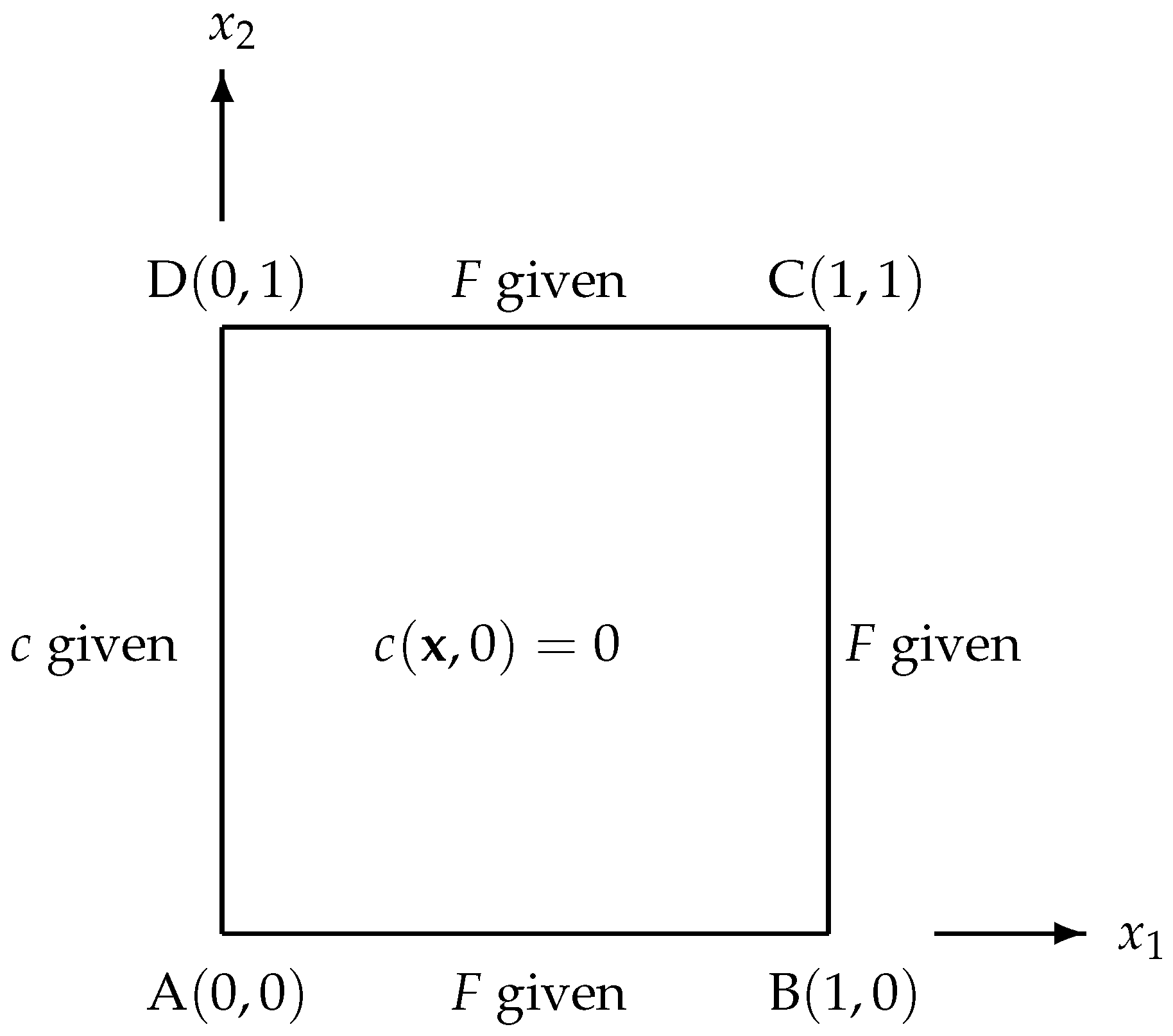
A standard BEM with constant elements is employed to obtain numerical results. For simplicity, a unit square depicted in Figure 1 and Figure 2 is taken as the geometrical domain for all problems. A total of 320 elements of equal length, namely 80 elements on each side of the unit square, are used.

A FORTRAN script is developed to compute the numerical solutions. A subroutine that evaluates the values of the coefficients $V_m,m=1,2,\dots ,N$ of the Stehfest formula in (38) for any number N is embedded in the script.

Table 1. Values of $V_m$ of the Stehfest formula for $N=6,8,10,12$.

${\mathit{V}}_{\mathit{m}}$	$\mathit{N}=6$	$\mathit{N}=8$	$\mathit{N}=10$	$\mathit{N}=12$
$V_1$	1	$-1/3$	$1/12$	$-1/60$
$V_2$	$-49$	$145/3$	$-385/12$	$961/60$
$V_3$	366	$-906$	1279	$-1247$
$V_4$	$-858$	16,394/3	−46,871/3	82,663/3
$V_5$	810	−43,130/3	505,465/6	−1,579,685/6
$V_6$	$-270$	18,730	−236,957.5	1,324,138.7
$V_7$		−35,840/3	1,127,735/3	−58,375,583/15
$V_8$		8960/3	−1,020,215/3	21,159,859/3
$V_9$			16,4062.5	−8,005,336.5
$V_{10}$			−32,812.5	5,552,830.5
$V_{11}$				−215,5507.2
$V_{12}$				359,251.2

shows the values of $V_m$ for $N=6,8,10,12$ resulting from the subroutine.

4.1. A Test Problem

The problems will consider three types of inhomogeneity functions $h\left(\mathbf{x}\right)$, namely the exponential function of form (41) with the compressible flow, and the quadratic and trigonometric functions of form (47) with incompressible flow. For all test problems, we take coefficients ${\widehat{d}}_{ij}$ and $\widehat{k}$

$${\widehat{d}}_{ij}=\left[\begin{array}{cc}1& 0.35\\ 0.35& 0.25\end{array}\right],\widehat{k}=0.5$$

(48)

and a set of boundary conditions (see Figure 1)

F is given on side AB, BC, CD

c is given on side AD

For each problem, numerical solutions of c and its derivatives $\partial c/\partial x_1$ and $\partial c/\partial x_2$ are sought at $19\times 19$ interior points $\left(x_1,x_2\right)=\left\{0.05,0.1,0.15,\dots ,0.9,0.95\right\}\times \left\{0.05,0.1,0.15,\dots ,0.9,0.95\right\}$ and 9 time-steps $t=0.0004,\frac{\pi }{8},\frac{\pi }{4},\frac{3\pi }{8},\frac{\pi }{2},\frac{5\pi }{8},\frac{3\pi }{4},\frac{7\pi }{8},\pi$. The value $t=0.0004$ is the approximating value of $t=0$ as the singularity of the Stehfest formula. The individual relative error $E_I$ at each interior point and the aggregate relative error $E_A$ of the numerical solutions are computed using the formulas

$$\begin{array}{ccc}\hfill E_I& =& \left|\frac{c_{n,i}-c_{a,i}}{c_{a,i}}\right|\hfill \end{array}$$

(49)

$$\begin{array}{ccc}\hfill E_A& =& {\left[\frac{{\sum }_{i=1}^{19\times 19}{\left(c_{n,i}-c_{a,i}\right)}^2}{{\sum }_{i=1}^{19\times 19}{c}_{a,i}^2}\right]}^{\frac{1}{2}}\hfill \end{array}$$

(50)

where $c_n$ and $c_a$ are the numerical and analytical solutions of c or its derivatives, respectively.

• Case 1:

First, we suppose that the function $h\left(\mathbf{x}\right)$ is an exponential function:

$$h\left(\mathbf{x}\right)={\left[exp\left(1+0.15x_1-0.25x_2\right)\right]}^2$$

(51)

that is, the material under consideration is exponentially graded material. We choose

$$\begin{array}{ccc}\hfill {\widehat{v}}_i& =& \left(1,1\right)\hfill \end{array}$$

(52)

$$\begin{array}{ccc}\hfill \widehat{\alpha }\left(t\right)& =& 0.192625t\hfill \end{array}$$

(53)

so that the system has a compressible flow, as the divergence of the velocity $v_i\left(x\right)$ does not equal zero. In order for $h\left(\mathbf{x}\right)$ to satisfy (41), then $\lambda =-0.088125$. The analytical solution $c\left(\mathbf{x},t\right)$ for this problem is

$$c\left(\mathbf{x},t\right)=\frac{texp\left[-\left(0.2x_1+0.3x_2\right)\right]}{exp\left(1+0.15x_1-0.25x_2\right)}.$$

(54)

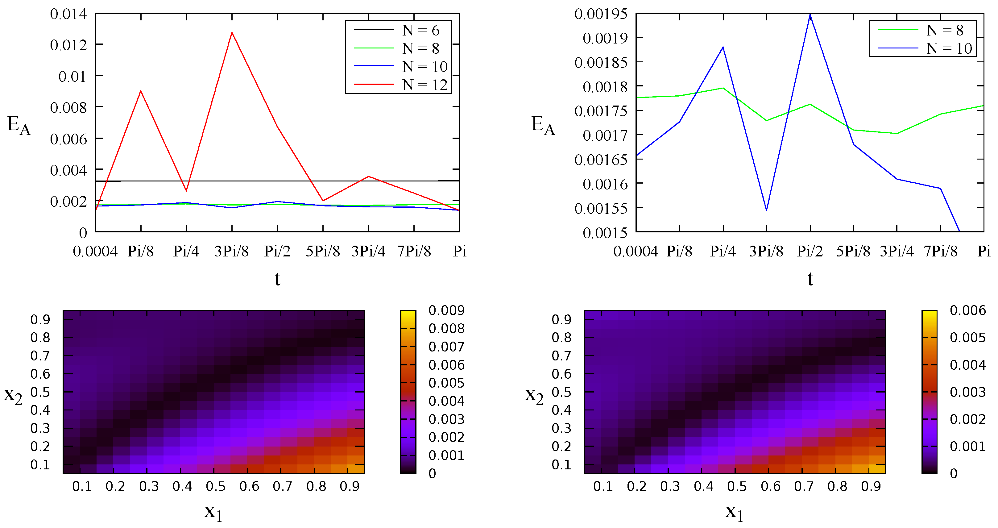
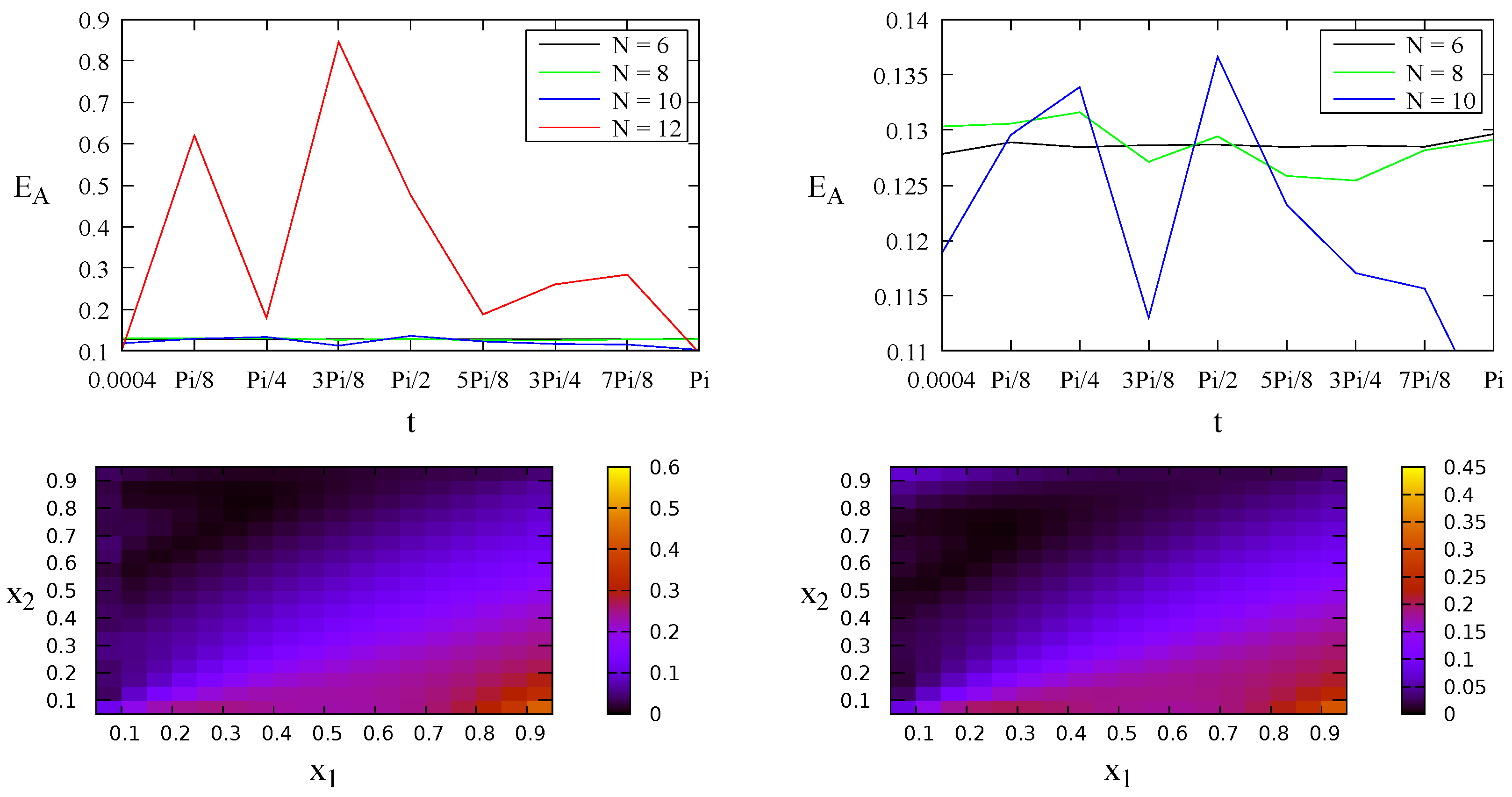
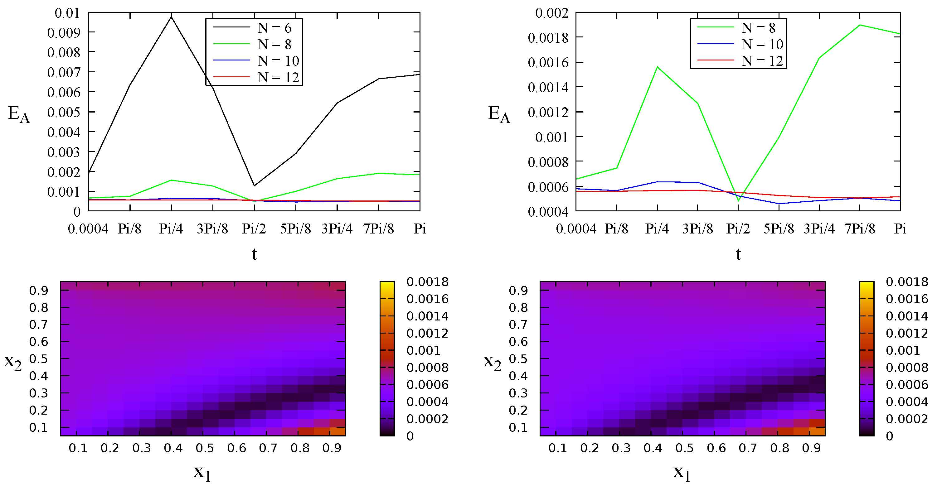
Figure 3 (top row) shows the aggregate relative errors $E_A$ of the numerical solutions c obtained using $N=6,8,10,12$ for the Stehfest formula (38). It indicates convergence of the Stehfest formula when the value of N changes from $N=6$ to $N=10$. For this specific case (Case 1), the value of N is optimized at $N=10$. Increasing N to $N=12$ does not give more accurate solutions. According to Hassanzadeh and Pooladi-Darvish [16], increasing N will increase the accuracy up to a point, and then the accuracy will decline due to round-off errors. The bottom row of Figure 3 depicts individual relative errors $E_I$ for the $19\times 19$ interior points at time $t=\pi /2$ (left) and $t=\pi$ (right), with $N=10$ as the optimized value of N. It indicates that the errors $E_I$ decrease as t changes from $t=\pi /2$ to $t=\pi$. This result agrees with the result of the aggregate relative error $E_A$ in the top row of Figure 3.

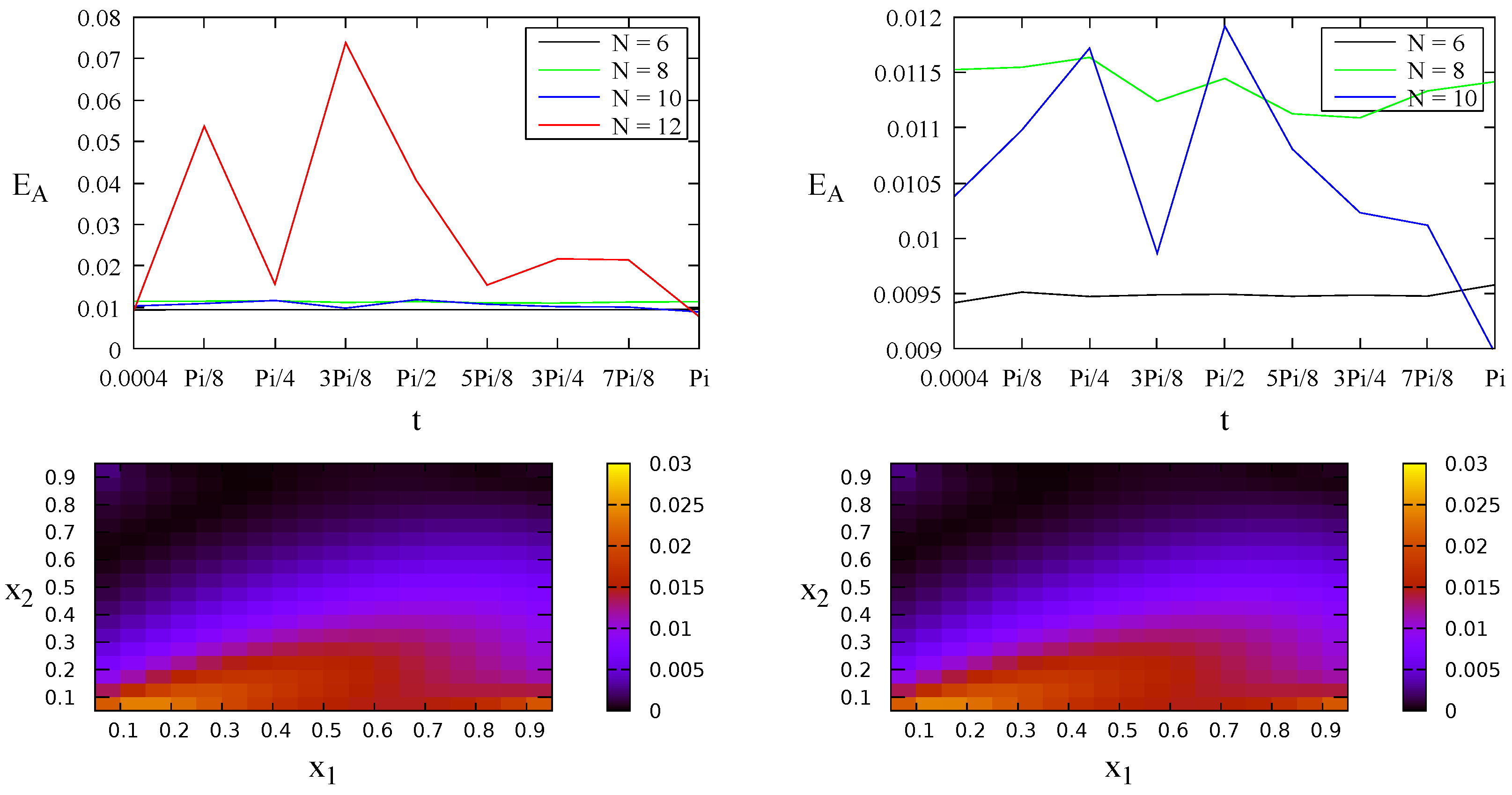
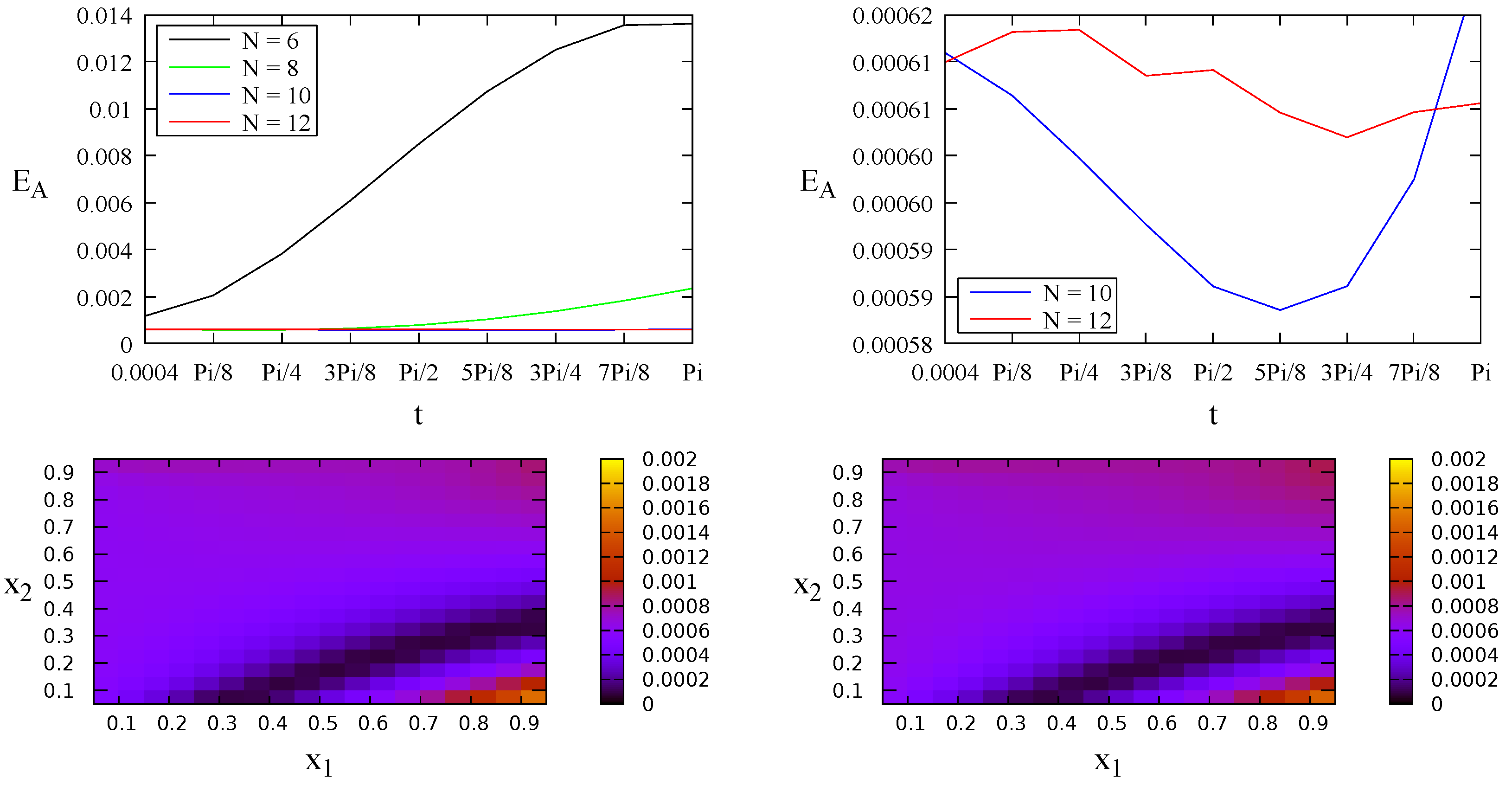
For the derivative solution $\partial c/\partial x_1$, Figure 4 (top row) shows that $N=6$ is the optimized value of N for the aggregate relative errors $E_A$. The bottom row of Figure 4 depicts individual relative errors $E_I$ with $N=6$. It indicates that the errors $E_I$ stay steady as t changes from $t=\pi /2$ to $t=\pi$. This result agrees with the result of the aggregate relative error $E_A$ in the top row of Figure 4.

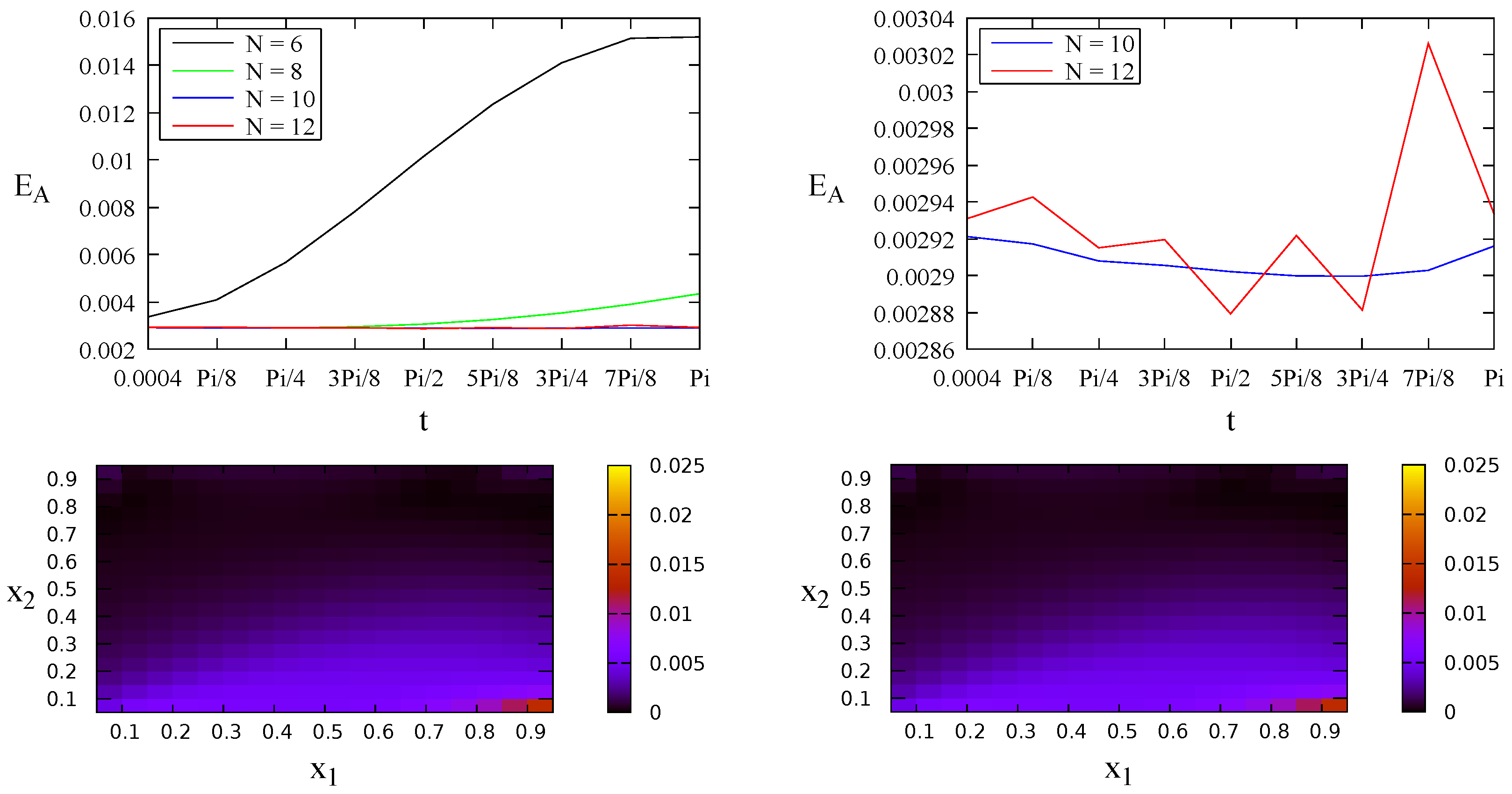
Meanwhile, for the derivative solution $\partial c/\partial x_2$, Figure 5 (top row) shows that $N=10$ is the optimized value of N for the aggregate relative errors $E_A$. The bottom row of Figure 5 depicts individual relative errors $E_I$ with $N=10$.

• Case 2:

Next, we choose an analytical solution:

$$c\left(\mathbf{x},t\right)=\frac{exp\left[-\left(0.2x_1+0.3x_2\right)\right]}{1+0.15x_1-0.25x_2}sin\sqrt{t}$$

(55)

Suppose the function $h\left(\mathbf{x}\right)$ and the coefficients are

$$\begin{array}{ccc}\hfill h\left(\mathbf{x}\right)& =& {\left(1+0.15x_1-0.25x_2\right)}^2\hfill \end{array}$$

(56)

$$\begin{array}{ccc}\hfill {\widehat{v}}_i& =& \left(1,0.6\right)\hfill \end{array}$$

(57)

$$\begin{array}{ccc}\hfill \widehat{\alpha }\left(t\right)& =& -0.031\sqrt{t}tan\left(\sqrt{t}\right)\hfill \end{array}$$

(58)

Therefore, the considered system involves a quadratically graded material with an incompressible flow. From (47), we have the parameter $\lambda =0$.

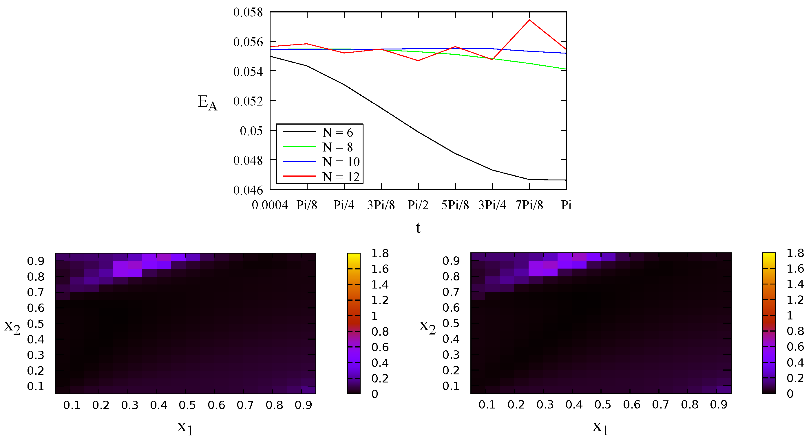
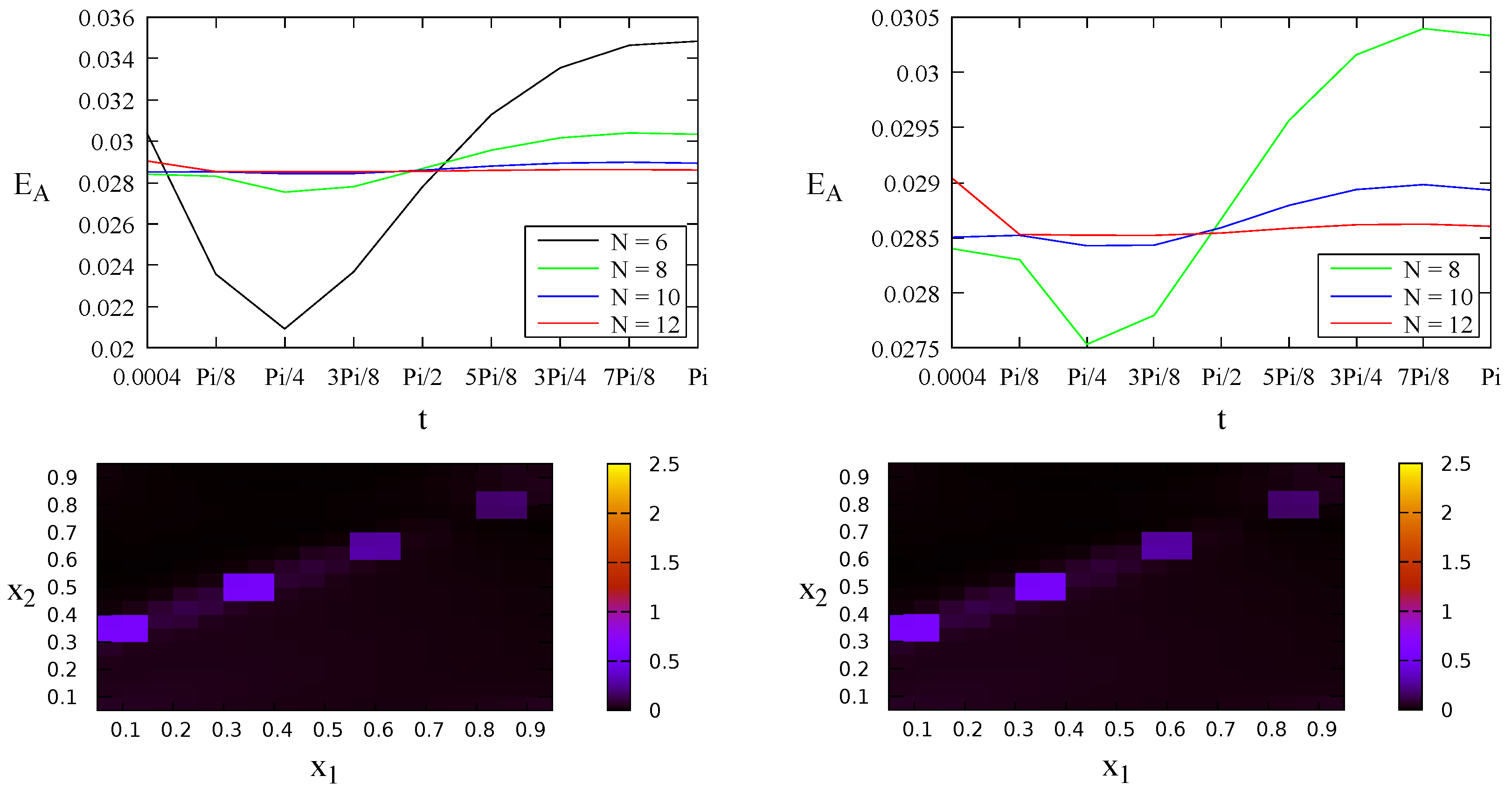
Figure 6 (top row) indicates that $N=10$ is the optimized value of N for the aggregate relative errors $E_A$ of the numerical solutions of c. Increasing N to $N=12$ gives worse solutions. The bottom row of Figure 6 depicts individual relative errors $E_I$ with $N=10$.

$N=10$ is also the optimized value of N for the aggregate relative errors $E_A$ of the numerical solutions $\partial c/\partial x_1$. This result is shown in Figure 7 (top row). The bottom row of Figure 7 depicts individual relative errors $E_I$ with $N=10$.

Meanwhile, for the derivative solution $\partial c/\partial x_2$, Figure 8 (top row) shows that $N=6$ is the optimized value of N for the aggregate relative errors $E_A$. The bottom row of Figure 8 depicts individual relative errors $E_I$ with $N=6$.

• Case 3:

Now, we consider a trigonometrically graded material with a grading function of

$$h\left(\mathbf{x}\right)={\left[cos\left(1+0.15x_1-0.25x_2\right)\right]}^2$$

(59)

We choose

$${\widehat{v}}_i=\left(1,0.6\right),\widehat{\alpha }\left(t\right)=0.003625\left[1-exp\left(t\right)\right]$$

(60)

so that the system has an incompressible flow, as the divergence of the velocity $v_i\left(x\right)$ equals zero. From (47) we have $\lambda =-0.011875$. The analytical solution of $c\left(\mathbf{x},t\right)$ for this problem is

$$c\left(\mathbf{x},t\right)=\frac{exp\left[-\left(0.2x_1+0.3x_2\right)\right]\left[1-exp\left(-t\right)\right]}{cos\left(1+0.15x_1-0.25x_2\right)}$$

(61)

Based on the results in Figure 9, Figure 10 and Figure 11 (top rows) we assume that $N=12$ is the optimized value for the aggregate relative errors $E_A$ of the solutions of c and the derivatives $\partial c/\partial x_1$ and $\partial c/\partial x_2$. The corresponding individual relative errors $E_I$ are shown in the bottom row of each figure.

4.2. A Problem without Analytical Solution

Further, we will show that the anisotropy and inhomogeneity of materials give an impact on the solutions. We will use ${\widehat{d}}_{ij},{\widehat{v}}_i,\widehat{k},h\left(\mathbf{x}\right)$ in Case 3 of Section 4.1 for this problem, which are

$$\begin{array}{ccc}\hfill {\widehat{d}}_{ij}& =& \left[\begin{array}{cc}1& 0.35\\ 0.35& 0.25\end{array}\right]\hfill \end{array}$$

(62)

$$\begin{array}{ccc}\hfill {\widehat{v}}_i& =& \left(1,0.6\right)\hfill \end{array}$$

(63)

$$\begin{array}{ccc}\hfill \widehat{k}& =& 0.5\hfill \end{array}$$

(64)

$$\begin{array}{ccc}\hfill h\left(\mathbf{x}\right)& =& {\left[cos\left(1+0.15x_1-0.25x_2\right)\right]}^2\hfill \end{array}$$

(65)

We choose

$$\widehat{\alpha }\left(t\right)=1$$

(66)

As we aim to show the impacts of anisotropy and inhomogeneity of the material, we need to consider the case of homogeneous material and the case of isotropic material. We assume that when the material is homogeneous, then

$$h\left(\mathbf{x}\right)=1$$

(67)

and when an isotropic material is under consideration, then

$${\widehat{d}}_{ij}=\left[\begin{array}{cc}1& 0\\ 0& 1\end{array}\right]$$

(68)

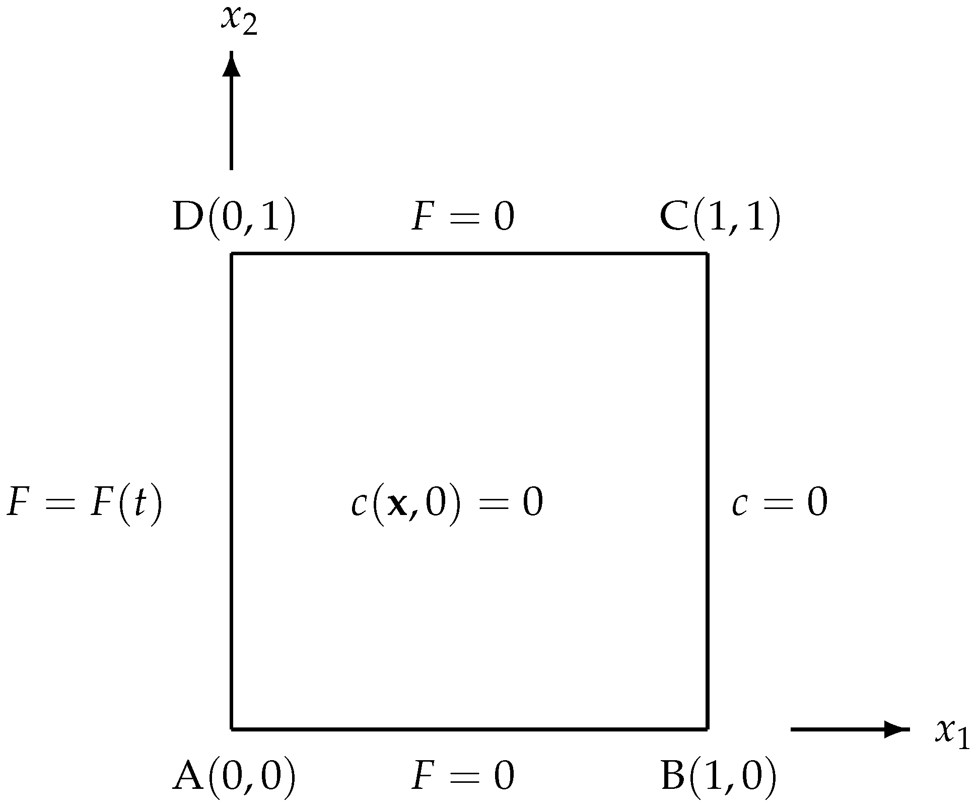
The boundary conditions are (see Figure 2)

$F=0$ on side AB

$c=0$ on side BC

$F=0$ on side CD

$F=F\left(t\right)$ on side AD

where $F\left(t\right)$ is associated with four cases, namely

Case 1:	$F\left(t\right)=1$
Case 2:	$F\left(t\right)=exp\left(-t\right)$
Case 3:	$F\left(t\right)=t$
Case 4:	$F\left(t\right)=t/\left(t+0.01\right)$

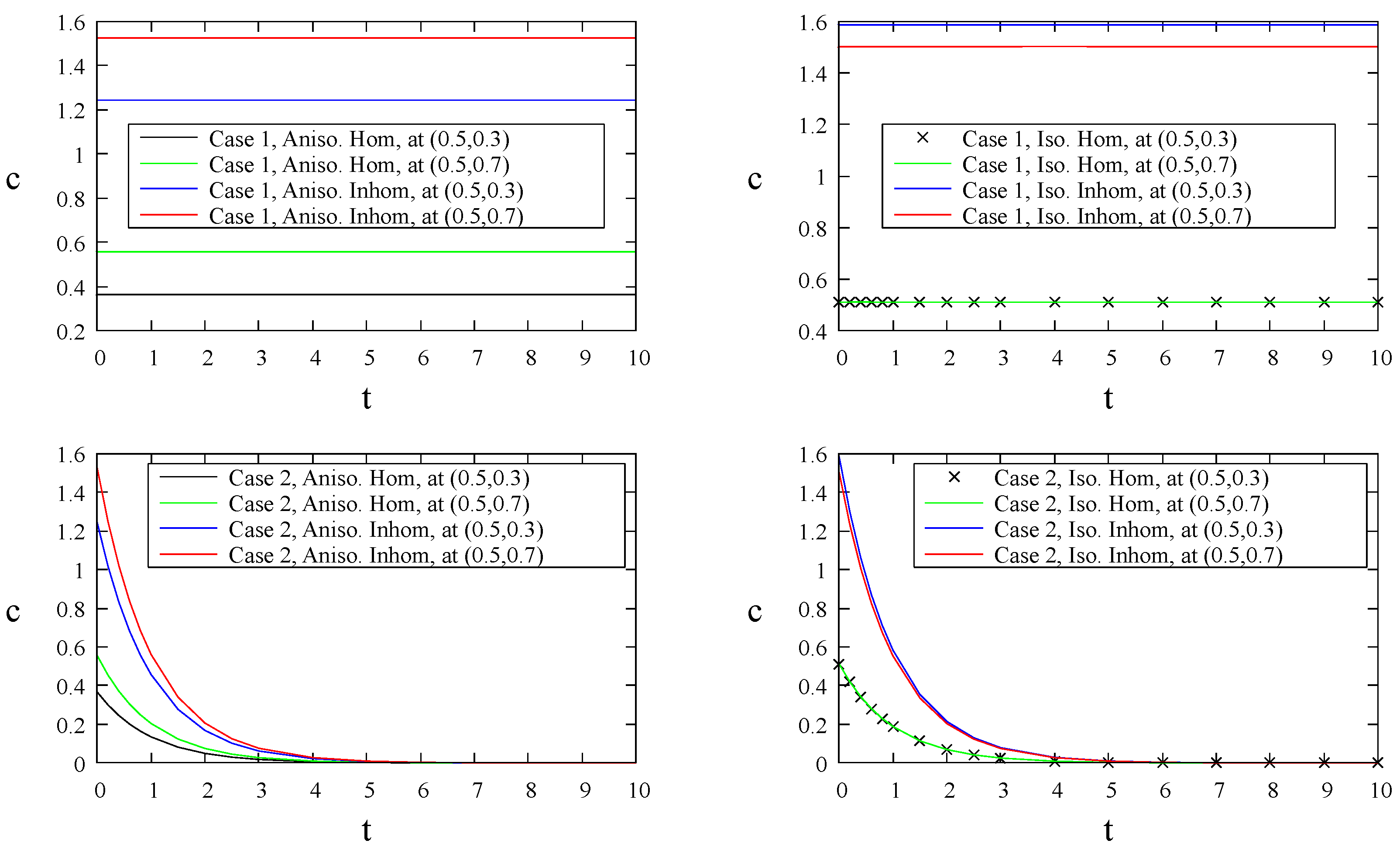
Figure 12 shows that for all cases, when the material is isotropic and homogeneous, the solutions $c\left(0.5,0.3,t\right)$ and $c\left(0.5,0.7,t\right)$ coincide. This is to be expected, as the problem is geometrically symmetric at $x_2=0.5$ when the material is isotropic and homogeneous. Furthermore, the results in Figure 12 also indicate that the material’s anisotropy and inhomogeneity affect the solutions. Once we change the material from homogeneous to inhomogeneous, or from isotropic to anisotropic, then the solution will not be symmetric anymore. Moreover, as is also expected, the variation of the solution with respect to t mimics the time function $F\left(t\right)$ as the boundary condition on side AD.

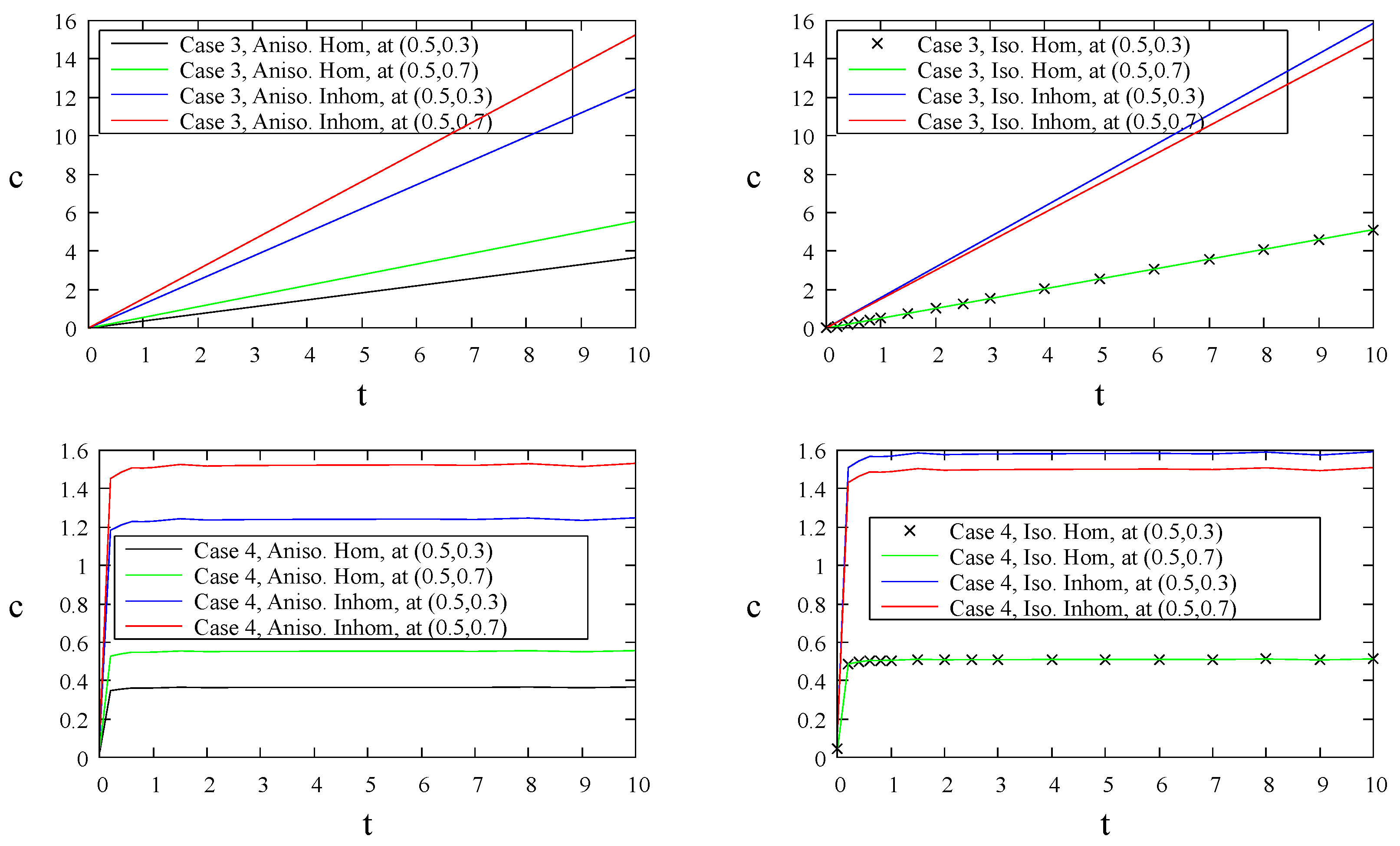
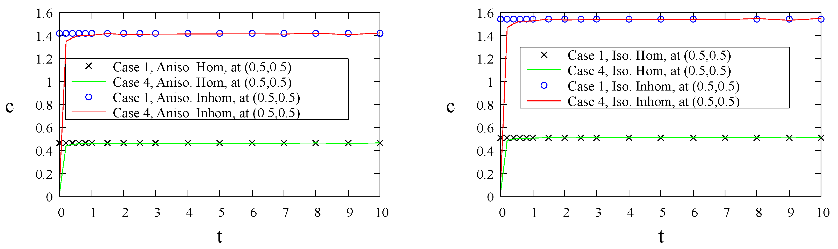
Meanwhile, the results in Figure 13 show that Case 1 of $F\left(t\right)=1$ and Case 4 of $F\left(t\right)=t/\left(t+0.01\right)$ have the same steady-state solution. This is to be expected, as both the functions $F\left(t\right)=1$ and $F\left(t\right)=t/\left(t+0.01\right)$ will converge to 1 when t approaches infinity.

5. Conclusions

Two-dimensional transient problems for anisotropic FGMs governed by a diffusion–convection–reaction equation of variable coefficients of the form (1) have been considered. The coefficients $d_{ij}\left(\mathbf{x}\right),v_i\left(\mathbf{x}\right),k\left(\mathbf{x}\right),\alpha \left(\mathbf{x},t\right)$ are restricted to take forms (5), (6), (7) and (8), respectively. By assuming that the gradation function $h\left(\mathbf{x}\right)$ satisfies (19), and by using the transformation (10), the variable coefficient Equation (1) is reduced to a constant coefficient Equation (20), which can be written in the form of the boundary-only integral Equation (35) and solved using a standard BEM for the solutions $c^{*}$. These BEM solutions are then numerically inverse transformed using the Stehfest formula (38) to obtain the solutions c.

Some problems of three types of gradation function $h\left(\mathbf{x}\right)$, namely trigonometric, exponential, and quadratic functions, have been solved. Based on the results obtained, we may conclude that the analysis of the reduction to the constant coefficient equation (in Section 3) for deriving the boundary-only integral Equation (35) is valid, and the combined BEM and Stehfest formula is quite accurate.

References

- Bear, J. Dynamics of Fluids in Porous Media; American Elsevier Publishing Company, Inc.: New York, NY, USA, 1972. [Google Scholar]
- Fredlund, D.G.; Rahardjo, H. Soil Mechanics for Unsaturated Soils; John Wiley & Sons: Hoboken, NY, USA, 1993. [Google Scholar]
- Charbeneau, R.J.; Sherif, S.A. Groundwater Hydraulics and Pollutant Transport. Appl. Mech. Rev. 2002, 55, B38–B39. [Google Scholar] [CrossRef]
- Yan, G.; Li, Z.; Galindo Torres, S.A.; Scheuermann, A.; Li, L. Transient Two-Phase Flow in Porous Media: A Literature Review and Engineering Application in Geotechnics. Geotechnics 2022, 2, 32–90. [Google Scholar] [CrossRef]
- Fendoglu, H.; Bozkaya, C.; Tezer-Sezgin, M. DBEM and DRBEM solutions to 2D transient convection-diffusion-reaction type equations. Eng. Anal. Bound. Elem. 2018, 93, 124–134. [Google Scholar] [CrossRef]
- Wang, X.; Ang, W.-T. A complex variable boundary element method for solving a steady-state advection–diffusion–reaction equation. Appl. Math. Comput. 2018, 321, 731–744. [Google Scholar] [CrossRef]
- Sheu, T.W.H.; Wang, S.K.; Lin, R.K. An Implicit Scheme for Solving the Convection–Diffusion–Reaction Equation in Two Dimensions. J. Comput. Phys. 2000, 164, 123–142. [Google Scholar] [CrossRef]
- Xu, M. A modified finite volume method for convection-diffusion-reaction problems. Int. J. Heat Mass Transf. 2018, 117, 658–668. [Google Scholar] [CrossRef]
- AL-Bayati, S.A.; Wrobel, L.C. Radial integration boundary element method for two-dimensional non-homogeneous convection–diffusion–reaction problems with variable source term. Eng. Anal. Bound. Elem. 2019, 101, 89–101. [Google Scholar] [CrossRef]
- Samec, N.; Škerget, L. Integral formulation of a diffusive–convective transport equation for reacting flows. Eng. Anal. Bound. Elem. 2004, 28, 1055–1060. [Google Scholar] [CrossRef]
- Rocca, A.L.; Rosales, A.H.; Power, H. Radial basis function Hermite collocation approach for the solution of time dependent convection–diffusion problems. Eng. Anal. Bound. Elem. 2005, 29, 359–370. [Google Scholar] [CrossRef]
- AL-Bayati, S.A.; Wrobel, L.C. The dual reciprocity boundary element formulation for convection-diffusion-reaction problems with variable velocity field using different radial basis functions. Int. J. Mech. Sci. 2018, 145, 367–377. [Google Scholar] [CrossRef]
- AL-Bayati, S.A.; Wrobel, L.C. A novel dual reciprocity boundary element formulation for two-dimensional transient convection–diffusion–reaction problems with variable velocity. Eng. Anal. Bound. Elem. 2018, 94, 60–68. [Google Scholar] [CrossRef]
- Hernandez-Martinez, E.; Puebla, H.; Valdes-Parada, F.; Alvarez-Ramirez, J. Nonstandard finite difference schemes based on Green’s function formulations for reaction–diffusion–convection systems. Chem. Eng. Sci. 2013, 94, 245–255. [Google Scholar] [CrossRef]
- Azis, M.I. Standard-BEM solutions to two types of anisotropic-diffusion convection reaction equations with variable coefficients. Eng. Anal. Bound. Elem. 2019, 105, 87–93. [Google Scholar] [CrossRef]
- Hassanzadeh, H.; Pooladi-Darvish, M. Comparison of different numerical Laplace inversion methods for engineering applications. Appl. Math. Comput. 2007, 189, 1966–1981. [Google Scholar] [CrossRef]
Figure 1.
The boundary conditions for problems in Section 4.1.
Figure 2.
The boundary conditions for problems in Section 4.2.
Figure 3.
(Top): The aggregate relative error of the numerical solutions of c with for Case 1 (left) and zoom-in view for (right). (Bottom): The individual relative errors at (left) and (right) with .
Figure 4.
(Top): The aggregate relative error of the numerical solutions with for Case 1 (left) and zoom-in view for (right). (Bottom): The individual relative errors at (left) and (right) with .
Figure 5.
Figure 6.
(Top): The aggregate relative error of the numerical solutions c with for Case 2 (left) and zoom-in view for (right). (Bottom): The individual relative errors at (left) and (right) with .
Figure 7.
(Top): The aggregate relative error of the numerical solutions with for Case 2 (left) and zoom-in view for (right). (Bottom): The individual relative errors at (left) and (right) with .
Figure 8.
(Top): The aggregate relative error of the numerical solutions with for Case 2. (Bottom): The individual relative errors at (left) and (right) with .
Figure 9.
(Top): The aggregate relative error of the numerical solutions of c with for Case 3 (left) and zoom-in view for (right). (Bottom): The individual relative errors at (left) and (right) with .
Figure 10.
(Top): The aggregate relative error of the numerical solutions with for Case 3 (left) and zoom-in view for (right). (Bottom): The individual relative errors at (left) and (right) with .
Figure 11.
Figure 12.
Solutions of and for all cases.
Figure 13.
Solutions of for Case 1 and 4.