Article

Finite-Element Method for the Simulation of Lipid Vesicle/Fluid Interactions in a Quasi–Newtonian Fluid Flow

Department of Mathematics, College of Arts and Sciences, Khalifa University of Science and Technology, Abu Dhabi P.O. Box 127788, United Arab Emirates
Mathematics 2023, 11(8), 1950; https://doi.org/10.3390/math11081950
Submission received: 17 March 2023 / Revised: 29 March 2023 / Accepted: 1 April 2023 / Published: 20 April 2023

Abstract

:
We present a computational framework for modeling an inextensible single vesicle driven by the Helfrich force in an incompressible, non-Newtonian extracellular Carreau fluid. The vesicle membrane is captured with a level set strategy. The local inextensibility constraint is relaxed by introducing a penalty which allows computational savings and facilitates implementation. A high-order Galerkin finite element approximation allows accurate calculations of the membrane force with high-order derivatives. The time discretization is based on the double composition of the one-step backward Euler scheme, while the time step size is flexibly controlled using a time integration error estimation. Numerical examples are presented with particular attention paid to the validation and assessment of the model’s relevance in terms of physiological significance. Optimal convergence rates of the time discretization are obtained.

1. Introduction

Motivated by their biomedical applications and their great potential for improving existing therapies, the development of accurate numerical tools to better understand the functioning processes of biomemetic lipid vesicles remains a dynamic and stimulating area of research [1]. They represent an attractif model system for a quantitative and predictive understanding of red blood cells (RBCs), whose dynamics continue to pose a formidable challenge to computational modeling [2]. Blood in the microvasculature is a complex fluid whose physiological behavior is critically dependent on its major cellular components, the RBCs. Although blood flow is generally assumed to be Newtonian fluid in the large vascular system, it exhibits a non-Newtonian shear-thinning rheology that cannot be overlooked at the microscopic scale, due to the complex mixture in the plasma [3,4,5,6,7]. Among several existing constitutive laws, we consider the Carreau’s constitutive law, commonly used for blood flow. That is, the viscosity exponentially decreases with increasing shear rates. A major challenge in complex flows lies in deciphering the fluid/membrane space-time interaction at the individual level [8]. Therefore, the simulation of such biomembranes needs to gain in accuracy. This work is oriented towards the direct numerical simulation of a deformable vesicle in a surrounding non Newtonian flow.
A variety of numerical methods have been developed for the vesicle problem by tracking explicitly (e.g., boundary integral method [9,10,11], immersed boundary method [12], penalty-immersed boundary method [13] lattice Boltzmann method [14], parametric finite element method [15,16], etc.) or implicitly (e.g., level set method [17,18,19,20,21], phase field approach [22,23], isogeometric phase field method [24], combined level set and phase field methods [25], etc.) the vesicle’s membrane. However, most numerical studies have been limited to Newtonian fluid models in the zero Reynolds limit. Nevertheless, an astonishing change in the RBC behaviors under finite Reynolds regimes was first pinpointed in [18,26]. To the best of our knowledge, the most relevant numerical study of the dynamics of a single Newtonian vesicle in a non-Newtonian fluid is presented in  [12], where an Oldroyd-B viscoelastic model was used to model the surrounding fluid of the vesicle.
To model the mechanical properties of the membrane of vesicles (and of biological membranes in general), a physiologically realistic model consists of the minimization of the scalar energy functional known as the Helfrich energy. In this model, the main mode of deformation is bending and the cost in bending is determined by the main curvatures of the membrane. That results in a highly nonlinear membrane force with respect to the shape. The model has been introduced in the early 1970s in separate works by Canham [27], Helfrich [28,29] and Evans [30]. For a phospholipidic membrane Γ , the Helfrich energy is expessed with respect to the mean curvature H as follows:
E ( Γ ) = k b 2 Γ H ( Γ ) 2 d s ,
with k b 10 20 kg m 2 s 2 the bending rigidity modulus [31,32]. Moreover, a phospholipid bilayer is purely fluidic interface characterized by the local inextensibility that constraints the surface divergence of the velocity field to vanish on the membrane. Membrane incompressibility plays an important role in the dynamics of flowing vesicles and leads to the preservation of the membrane surface (or perimeter in two-dimensional studies) thanks to Reynolds’ lemma, see [18]. This constraint can be enforced, for example, via an exact Lagrange multiplier localised on the membrane which can be thought of as a position-dependent membrane tension [33] or an elastic force expressed in terms of membrane stretching [17]. The fluid/membrane coupling remains challenging due to the highly nonlinear membrane force with respect to the the shape of the vesicle. Instead of using a body-fitted grid for the membrane description, we employ a level set Eulerian framework for a straightforward representation of the sharp interface with a signed distance function [34,35,36]. Generally speaking, the level set method makes it possible to naturally handle the topological changes of interfaces such as interface merging or breaking. On the contrary, numerical problems related to the mesh distortion can raise when modeling the large displacement of an interface or topological changes using Lagrangian approaches. Special treatments and remeshing procedures are required in such situations, which generally remain difficult. The mechanics of the membrane is introduced through a localized body-force term [19]. The deflation of the vesicles is quantified by a dimensionless geometric parameter: the reduced area
v = ( A / π ) ( P / 2 π ) 2 1 ,
with P the perimeter of the vesicle and A the area of the enclosed subdomain.
We have arranged the remainder of the article as follows. Section 2 presents the mathematical framework for an individual vesicle immersed in a non-Newtonian Carreau fluid and the nonlinear coupled problem. It also introduces the penalty method and details the variational formulation of the problem. Section 3 is devoted to the time discretization scheme and provides the global algorithm used in the numerical simulations. In Section 4, we report sample numerical simulations in the Newtonian and non-Newtonian cases with some validation results to illustrate the accuracy of the method. The conclusion and future research directions are presented in Section 5.

2. Problem Statement

The spatio-temporal deformations of the vesicle are driven by the bending force, actions of fluid forces and boundary conditions, requiring the balance equations of mass and momentum. The fluid-membrane coupling is described through the balance of hydrodynamic stress by the bending response of the membrane. The level set description of the membrane obeys a Hamilton–Jacobi equation.

2.1. Level Set Formulation

Let T > 0 and for any time t ( 0 , T ) , consider a 2D vesicle Γ ( t ) = Ω ( t ) immersed in a non Newtonian fluid occupying both extracellular Λ \ Ω ( t ) and enclosed Ω ( t ) spaces. Here, Λ R 2 is a bounded convex polygonal domain with Γ ( t ) Λ = . See Figure 1. From now, the explicit dependence of Γ ( t ) and Ω ( t ) from time will be understood but will be omitted.
The membrane is implicitely described as a zero-level set of a Lipschitz continuous scalar function as follows
Γ = ( t , x ) ( 0 , T ) × Λ : φ ( t , x ) = 0 .
We assume that the region with negative φ ( t , . ) represents the internal domain of the vesicle Ω . Generally speaking, the main utility of an implicit representation of an interface is that large deformations or changes in topology, such as merging or pinching, which frequently occur when dealing, for example, with bubbles and drops, can be treated in a natural and direct way without the need for meshing or local refinement of the mesh in the vicinity of the complex interface; Authomatic meshing remains challenging especially in three-dimensional setups. The level set function is initialized as a signed distance function φ 0 with respect to the initial position of the vesicle Γ . It is given by
φ 0 ( x ) = inf y Γ ( 0 ) y x , if x Ω ( 0 ) inf y Γ ( 0 ) y x , otherwise .
Let I be the identity tensor. Geometric quantities, such that the unit normal outward vector n = φ / | φ | , the mean curvature H = div n , the surface projector π Γ = I n n , as well as the surface gradient s = π Γ , the surface divergence s · = tr ( s ) and the surface Laplacian Δ s operators are encoded in terms of φ . These quantities are consequently extended to the entire computational domain Λ . The Helfrich force requires a fourth-order derivative of φ , yielding a numerically stiff problem with severe time-step limitations needed for stability [33,37].

2.2. Fluid Constitutive Equations

Let u and p be the fluid velocity and pressure fields. Consider a quasi Newtonian constitutive law, where the Cauchy stress
σ = 2 η D ( u ) 2 D ( u ) p I
is expressed with respect to the rate-of-strain
D ( u ) = 1 2 ( u + u T ) .
Let us consider the Euclidean norm of tensors | τ | = ( 1 2 τ : τ ) 1 / 2 . The shear rate is then given by | 2 D ( u ) | . The shear-rate dependent viscosity follows the Carreau’s law
η γ = η + ( η 0 η ) 1 + κ γ ς 1 2 ,
with γ R + , η 0 η > 0 ; See ([38] Section 2.1, Definition 2.3). Note that we followed the notations in ([38] Definition 2.5), where the viscosity function is expressed with respect to the square of the shear rate γ = | 2 D ( u ) | 2 , instead of the shear rate directly. Blood flow features a shear thinning behavior, that is ς < 1 , which implies that the viscosity decreases with the shear rate. We consider the physiological parameters of human blood (assuming a hematocrit concentration 45 % at an ambient temperature 37 ), obtained by fitting data from normal blood samples in [4]. We assume piecewise constant zero-shear viscosity η 0 = μ i and η 0 = μ o = 0.16 Pa s in the enclosed Ω and surrounding Λ \ Ω subdomains, respectively.  The latter correspond to the viscosities in the Newtonian case ς = 1 . Without loss of generality, we assume equal infinite shear viscosities η = 0.0035 Pa s of the inner and outer fluids.
A linear shear flow is characterized by the imposition of a no-slip condition with constant opposing velocity u = u b on the horizontal boundaries Σ D of a square domain, while stress-free boundary conditions are prescribed elsewhere on Σ N = Λ \ Σ D  [39].
Although φ is initialized as a signed distance function with respect to the membrane of the vesicle, the advection of the level set function degenerates its initial signed distance property and the norm of the level set gradient may locally vanish or blow up, resulting in numerical singularities. This issue is worked around by solving an auxiliary redistancing equation which helps recover the original signed distance behavior [34,40]. Only a few redistancing iterations are usually done on a regular basis, as the level set function must be kept close to a signed distance map and not necessarily an exact distance, see, e.g., [37].
Three dimensionless physical parameters arise: The Reynolds number Re compares the strength of inertial forces to the viscosity effect. The bending number Bn relates the force of the imposed flow to the characteristic membrane bending strength. The viscosity contrast μ ¯ = μ i / μ o varies by changing the viscosity of the inner fluid and is relevant for the vesicle’s dynamics. Equal densities are assumed in inner and outer domains as this has no effect on the dynamics of the BRC [41]. We introduce the smoothed Heaviside H ε ( · ) and Dirac δ ε ( · ) functions within a banded strip of width 2 ε > 0 around Γ for easy approximations of integrals. They regularized functions are given by
H ε ( φ ) = 0 , if   φ < ε 1 2 1 + φ ε + sin π φ ε π , if   φ ε 1 , otherwise , δ ε ( φ ) = d H ε d φ ( φ ) = 1 2 ε 1 + cos π φ ε , if   φ ε 0 , otherwise .
The standard finite element approximation would result in suboptimal convergence due to the level set regularization. See for example [42] for more details on this issue.
From now, all quantities are non-dimensionalized. The same notations will be used for ease of exposition. The normalized regularized viscosity is expressed as
η ε ( γ , φ ) = η + H ε ( φ ) + μ ¯ 1 H ε ( φ ) η 1 + κ γ ς 1 2 , with γ > 0 .

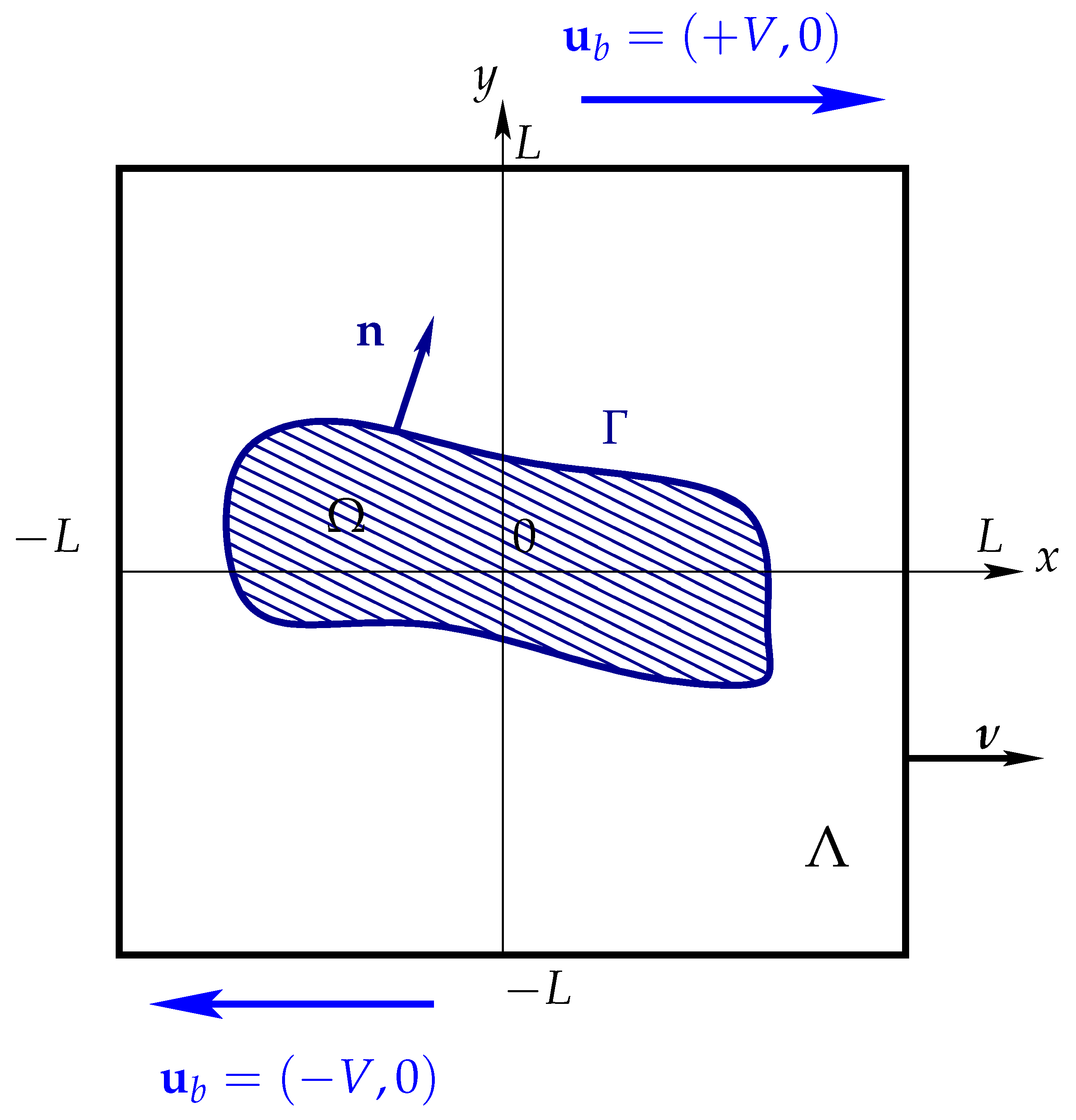
2.3. Statement of the Fluid-Vesicle Interaction Problem

Assume fluid incompressibility (mass conservation (2c)). Completed with the conditions of continuity and mechanical equilibrium at the interface, the normalized coupled fluid/membrane problem takes the form: Find φ , u , p and λ such that
φ t + u . φ = 0 , ( 0 , T ) × Λ ,
Re u t + u . u · η ε | 2 D ( u ) | 2 , φ + p = 0 , ( 0 , T ) × Λ ,
. u = 0 , ( 0 , T ) × Λ ,
s . u = 0 , ( 0 , T ) × Γ .
Let [ [ · ] ] be the discontinuity jump of a given field across the vesicle membrane Γ in its normal direction n . The system (2a–2d) is endowed with the conditions of continuity and mechanical equilibrium at the interface
[ [ u ] ] = 0 ,
[ [ σ n ] ] = s λ λ H n + 1 Bn 2 Δ s H + H 3 2 n .
The latter is transferred as a source term in the momentum equation. We refer to [18] for more details on the total stress jump across the vesicle and the derivation of the membrane bending force. Moreover, we consider the boundary conditions φ = φ b and u = u b on ( 0 , T ) × Σ , and σ · n = 0 on ( 0 , T ) × Σ N . Here Σ ( t ) = { x Λ : u ( t , x ) · ν ( x ) < 0 } is the inflow and ν is the outward-pointing unit normal to Λ , see Figure 1.

2.4. Panalty Approach

For the shear flow setups, we introduce V ( u b ) = { v ( H 1 ( Λ ) ) 2 : v = u b   on   Σ D } . Hence, the admissible velocities belong to the constrained space
K ( u b ) = v V ( u b ) : . v = 0   in   Λ , s . v = 0   in   Γ .
Analogously to the pressure p introduced to impose the incompressibility of the fluid, the zero surface divergence constraint (2d) is imposed by an exact local Lagrange multiplier λ on Γ  [33]. Targeting reduced computational load and simple implementation using standard fluid solvers, a penalty method relaxes the inextensibility constraint. For ease of presentation, the penalized problem is presented for vanishing inertia. The unsteady case can be written after time discretization, see a detailed presentation for a different problem in [43]. Let us introduce the dimensionless sharp function:
η 0 * ( t , x ) = μ ¯ when   x Ω ( t ) , 1 otherwise   for   Λ \ Ω ( t ) .
The problem (2) is first witten as a minimization under constraint:
( u , Ω ) = arg inf v K ( t , u b ) , ω Λ J ( v , ω ) ,
with a total energy functional
J ( v , ω ) = Λ J | 2 D ( u ) | 2 d x + 1 2 Bn ω H 2 ( ω ) d s .
Here, the scalar differentiable energy of dissipation reads
J ( γ ) = η 2 γ + ( η 0 * η ) κ ( ς + 1 ) ( 1 + κ γ ) ς 1 2 1 .
Note that the Helfrich energy term depends indirectly on the velocity field u , since the function φ describing the shape, is advected by u . The optimality system results from a saddle-point formulation. To alleviate the inextensibility, we introduce the space of unconstrained incompressibility
K ˜ ( u b ) = { v = u b : · v = 0   in   Λ }
For a small penalty parameter ϵ , the minimization problem (5) is approached by another minimization problem penalizing (2d):
( u , Ω ) = arg inf v K ˜ ( t , u b ) ω Λ J ϵ ( v ) = J ( v ) + 1 ϵ ω s · v 2 d s .
Using a saddle point formulation, the optimality system produces a penalty term in the momentum equation. The level set advection equation is solved by the Streamline Upwind Petrov-Galerkin method, with a stabilisation term S ( φ , ψ ) introducing diffusion in the streamline direction [19].
Spatial discretization is carried out by finite elements. To reduce spurious oscillations and errors due to multi-space projections for lower degree polynomials and accurately calculate the bending term, higher order finite elements are considered using Lagrange polynomials of degrees k + 1 , k and k + 1 for u , p and φ , respectively, with k = { 1 , 2 , 3 } . Considering the total derivative term, the variational formulation of the panalized problem writes:
Find u C 0 ( ( 0 , T ) , V ( u b ) ) , p L 2 ( ( 0 , T ) , L 0 2 ( Λ ) ) and φ C 0 ( ( 0 , T ) , W 1 , Λ H 1 ( Λ ) ) such that
Re Λ u t + u · u · v + Λ 2 η ε | 2 D ( u ) | 2 , φ D ( u ) : D ( v ) Λ p . v
+ 1 ϵ Λ | φ | δ ε ( φ ) ( s . u ) ( s . v ) 1 Bn Λ | φ | δ ε ( φ ) Ψ + H 3 2 n · v = 0 ,
Λ q . u = 0 ,
Λ | φ | Ψ ξ + Λ | φ | s H · s ξ = 0 ,
Λ φ t ψ + Λ u · φ ψ + Λ S φ , ψ = 0 ,
v V ( 0 ) , q L 0 2 ( Λ ) , ξ H 1 ( Λ )   and   ψ H 1 ( Λ ) .

3. Time Discretization

We consider a first order backward Euler scheme, referred to as BE, usually used for the vesicle’s problem, and rely on the flow composition technique to raise the order of the time integration scheme [44]. An adaptive time-stepping will be introduced afterwards.

3.1. Error Estimation

Henceforth, we focus on the time discretization of the system of first-order differential equations obtained by finite element discretization. It is simply denoted by
y = f ( t , y ( t ) ) , with y ( 0 ) = y 0 and t R .
Assume f is an analytic function. Let t n , 0 n N be a partition of the time interval [ 0 , T ] with time step δ t = t n + 1 t n . and y n be the approximations of the solution y ( t n ) . Let 𝓨 t : R R be the exact t-flow of the above differential equation so that with 𝓨 t ( y 0 ) = y ( t ) . A basic integrator, such that y n + 1 = Y δ t ( y n ) , is said of order p if the following equation holds
𝓨 δ t ( y 0 ) Y δ t ( y 0 ) = O δ t p + 1 .
The order p of a one-step method can be raised by composition Y a 1 δ t Y a s δ t with step sizes a 1 δ t , , a s δ t to at least an order p + 1 if the conditions
a 1 + + a s = 1 and a 1 p + 1 + + a s p + 1 = 0
are satisfied [44]. No real solutions hold for odd p; This can be circumvented by considering, for instance, an analytic continuation off the real axis by using complex coefficients a i ’s [45]. For a thorough description of the composition of multi-step methods and the choice of parameters a 1 , , a s for any general order p and step number s, we refer to the book ([44] Section II.4).
In what follows, we limit our approach to the double composition (i.e., we set s = 2 ) of the numerical flow Y δ t associated with the backward Euler scheme, that is
Y δ t ( y n ) = y n + δ t f ( t n , y n ) .
The aforementioned algebraic conditions provide the coefficients 2 a 1 = 2 a ¯ 2 = 1 + i .
Theorem 1.
For n 0 , consider the first order differential equations in [ t n , t n + 1 ] . Let us denote y n + 1 , 0 = y n , y n + 1 , 1 = Y a 1 δ t y n + 1 , 0 and y n + 1 , 2 = Y a 2 δ t y n + 1 , 1 = Y a 2 δ t Y a 1 δ t y n . The composed method defined by the real part y n + 1 = Re y n + 1 , 2 is a numerical method of order 2. Furthermore, the imaginary part, referred to as Im y n + 1 , 2 , represents an error estimate of the approximation to within O δ t 3 .
Proof. 
For n 1 and k = 1 , 2 , we shall expand f ( t n + a k δ t , y n + 1 , k ) into a Taylor series around ( t n , y n + 1 , k 1 ) . We have
y n + 1 , 1 = y n + 1 , 0 + a 1 δ t f t n , y n + 1 , 0
and
y n + 1 , 2 = y n + 1 , 1 + a 2 δ t f t n + a 1 δ t , y n + 1 , 1 .
Considering y n + 1 , 2 , we expand the right-hand expression into a Taylor series and truncate
y n + 1 , 2 = y n + 1 , 1 + a 2 δ t f t n + a 1 δ t , y n + 1 , 1 = y n + a 1 δ t f ( t n , y n ) + a 2 δ t f t n + a 1 δ t , y n + a 1 δ t f ( t n , y n ) = y n + a 1 δ t f ( t n , y n ) + a 2 δ t [ f ( t n , y n ) + a 1 δ t f t + f f y ( t n , y n ) . + 1 2 a 1 2 δ t 2 f t , t + 2 f t , y f + f y , y f 2 ( t n , y n ) + O δ t 3 ] = y n + ( a 1 + a 2 ) δ t f ( t n , y n ) + ( a 1 a 2 ) δ t 2 f t + f y f ( t n , y n ) + 1 2 a 2 a 1 2 δ t 2 f t , t + 2 f t , y f + f y , y f 2 ( t n , y n ) + a 2 δ t O δ t 3 .
The subscript refers to the partial derivatives with respect to the given variable. Using the expression of y ( 2 ) , we get
y n + 1 , 2 = y n + ( a 1 + a 2 ) δ t y ( t n ) + ( a 1 a 2 ) δ t 2 y ( t n ) + 1 2 a 2 a 1 2 δ t 2 f t , t + 2 f t , y f + f y , y f 2 ( t n , y n ) + O δ t 4 .
The coefficients a 1 and a 2 satisfy a 1 + a 2 = 1 and 2 a 1 a 2 = 1 . Thus, one can write y n + 1 , 2 = Re y n + 1 , 2 + i Im y n + 1 , 2 . The real part of the approximated solution reads
Re y n + 1 , 2 = Re y n + δ t y ( t n ) + 1 2 δ t 2 y ( t n ) + 1 4 δ t 3 a 1 f t , t + 2 f t , y f + f y , y f 2 ( t n , y n ) + O δ t 4 ) = Re y n + δ t y ( t n ) + 1 2 δ t 2 y ( t n ) + Re a 1 δ t 3 4 f t , t + 2 f t , y f + f y , y f 2 ( t n , y n ) + Re O δ t 4 = y n + δ t y ( t n ) + δ t 2 2 y ( t n ) + δ t 3 8 f t , t + 2 f t , y f + f y , y f 2 ( t n , y n ) + Re O δ t 4 .
By using the Taylor expansion of the exact solution y ( t n + 1 ) at the vicinity of t n and the expressions of the higher derivatives of the solution, we evaluate the error between the exact solution and Re y n + 1 , 2 as follows
e ( t n + δ t ) = y ( t n + 1 ) Re y n + 1 , 2 = δ t 3 24 y ( 3 ) ( t n ) + δ t 3 8 f t f y + f y 2 f ( t n , y n ) + Re O δ t 4 .
As a consequence, the composed scheme is indeed convergent and of second-order, provided f and its derivatives are bounded. Furthermore, the imaginary part of y n + 1 , 2 is expressed as follows:
Im y n + 1 , 2 = Im a 1 δ t 3 4 f t , t + 2 f t , y f + f y , y f 2 ( t n , y n ) + Im O δ t 4 = δ t 3 8 y ( 3 ) ( t n ) + δ t 3 8 f t f y + f y 2 f ( t n , y n ) + Im O δ t 4 .
By taking the difference between the error in (9) and the imaginary part of y n + 1 , 2 , we end up with
e ( t n + δ t ) Im y n + 1 , 2 = δ t 3 6 y ( 3 ) ( t n ) + O δ t 4 ,
As a matter of fact, the imaginary part denoted in the sequel by ζ n + 1 = Im y n + 1 , 2 , is an approximation of the error up to third order and represents an error estimate of the approximated solution y n + 1 = Re y n + 1 , 2 .    □

3.2. Time-Stepping Strategy

The vesicle can undergo more or less rapid dynamics or deformations over time. Although using a uniformly large time step can produce unphysical solutions and numerical instabilities, using larger time steps for some slow dynamics (e.g., around the horizontal position during tumbling) improves the computational efficiency. In [33], a manual adjustment is introduced to improve the quadratic convergence of the Newton’s algorithm. In this work, we adopt an adaptive time stepping scheme where the time step size is flexibly controlled such that the time integration error, estimated by ζ n at t n , does not exceed a prescribed threshold value. Let δ t m a x and δ t m i n be the upper and lower bounds of δ t , generally chosen as 10 1 and 10 3 for the vesicle problem. Let C be a predefined parameter introduced to calibrate the level of adaptability, while 10 α with α > 0 is the desired precision and p represents the order of the method. The variable time step δ t n + 1  reads:
δ t n + 1 = δ t n 10 k C ζ n + 1 L 2 ( Λ ) 1 / p .
Following [46], we also perform a comparison with a known criterion based on the the change rate of two consecutive numerical solutions δ t φ n . For a predetermined constant C = 10 3 , the adapted step size is given by:
δ t n + 1 = max δ t m i n , δ t m a x 1 + C δ t φ n L 2 ( Λ ) 2 .

3.3. Overall Algorithm

The membrane and fluid problems are first solved iteratively, while a fixed-point loop allows a strongly coupled approach for better numerical stability. Indeed, the level set problem is first solved using the velocity in the previous iteration; the fluid problem is subsequently solved using the updated level set function in the membrane force calculation. Fixed point convergence is reached when the absolute error between two subsequent iterates is less than a prescribed tolerance, set tol = 10 6 in the calculations. The overall coupling approach is detailed in Algorithm 1.
Algorithm 1 Fluid/vesicle coupling algorithm
1:
Set fixed-point tolerance tol and time step δ t 0
2:
Set initial conditions ( n = 0 ): u 0 and φ 0 are known values
3:
for  n = 0 , , n max  do
4:
   Update time t n + 1 = t n + δ t n
5:
   Set, from known values, u n + 1 0 = u n and φ n + 1 0 = φ n
6:
   for  k = 0 , , k max  do
7:
     Compute φ n + 1 k + 1 from (7d), advected with velocity u n + 1 k
8:
     Compute the mixed variable Ψ  (7c) and membrane force in (7a) with φ n + 1 k + 1
9:
     Compute u n + 1 k + 1 and p n + 1 k + 1 by solving the linear generalised Stokes subproblem (7a) and (7b)
10:
     Compute absolute error err k + 1 : = H ε φ n + 1 k + 1 H ε φ n + 1 k L 2 ( Ω )
11:
     if  err k + 1 < tol  then
12:
        Update solution u n + 1 = u n + 1 k + 1 , p n + 1 = p n + 1 k + 1 and φ n + 1 = φ n + 1 k + 1
13:
        break
14:
     end if
15:
   end for
16:
   if  t n + 1 T  then
17:
     break
18:
   end if
19:
   Compute the adapted time step δ t n + 1 with φ n + 1
20:
end for

4. Numerical Results and Discussion

We provide several validation tests to illustrate the accuracy in terms of spatial and temporal convergence and the ability of the model to predict experimentally observed outcomes, including vesicle regimes under simple shear flow in purely Newtonian flow.
The simulations have been run using the C++ library for scientific computing Rheolef [47], with particular emphasis on finite elements and parallel computing. The calculations were performed on non-regular meshes generated using Gmsh (GMSH– http://www.geuz.org/gmsh (accessed on 28 March 2023)). Figures are generated using Paraview (Paraview–http://www.paraview.org (accessed on 28 March 2023)) and Gnuplot (Gnuplot–http://www.gnuplot.info (accessed on 28 March 2023)).

4.1. Verification of the Method–Time Convergence

In this test case, we use numerical simulations to verify the above analytical results, mainly in terms of convergence behavior. We first test the accuracy of the time integration scheme and the composition method by solving the following initial value problem
y + tan ( t 2 ) y = 2 a ( t 2 ) cos ( t 2 ) ( a ( t 1 ) ( t 3 ) ) 2 + 1 , y ( 0.5 ) = y 0 .
The exact solution
y ( t ) = cos ( t 2 ) arctan a ( t 1 ) ( t 3 )
has stiff variations at t = 1 and t = 3 which are calibrated by the parameter a. The initial condition y 0 is given by the exact solution evaluated at t = 0.5 . We solve the differential equation numerically over the time interval [ 0.5 , 6 ] using different numerical schemes for a relatively large stiffness coefficient a = 50 .
We consider constant time step sizes and perform a convergence study for the first-order basic BE, the double composition of BE, the second-order Cranck Nicolson (simply denoted by CN) versus successively refined step sizes δ t . The log-log plot of errors with respect to the exact solution in the norm l is reported in Figure 2 as a function of δ t . Results corroborate the theoretical time rates of convergence, showing first-order and second-order convergences for BE and CN, respectively, while a higher quadratic convergence is achieved by dual composition of BE scheme. Moreover, a high order cubic convergence is obtained by double composition of the composed BE scheme. Consequently, the error bounds are of optimal order in time.
We now proceed to a quantitative comparison between the time-stepping strategies. The initial value problem is solved using adapted time steps generated using both the error estimate ζ n and the rate of change criterion. The calculations are also performed with a constant time step δ t * so as to perform the same number of iterations as in the case of the adaptation of δ t with the criterion ζ n . Results are reported in Figure 3a–c.
Figure 3c highlights the need to use an adapted time step according to the variations of the solution in order to obtain an accurate evaluation in areas of stiff variations. Visually, one perceives significant discrepencies compared to the exact solution, which is not the case for calculations with the adapted time steps.
We give on Figure 3a the evolution over time of the adapted time steps δ t n using for the adaptation the two criteria above: the error estimate ζ n and rate of change | δ t ( y n ) | . Although there is overall agreement in terms of variations of the adapted time steps, the ζ n criterion makes it possible to capture the stiff variations with an appropriate level of temporal adaptability compared to the rate of change. Indeed, we plot on Figure 3c the error with respect to the exact solution as a function of time, showing clearly better accuracy when using ζ n compared to the criterion | δ t ( y n ) | , which provides better results compared to the compuations with a constant time step δ t * .

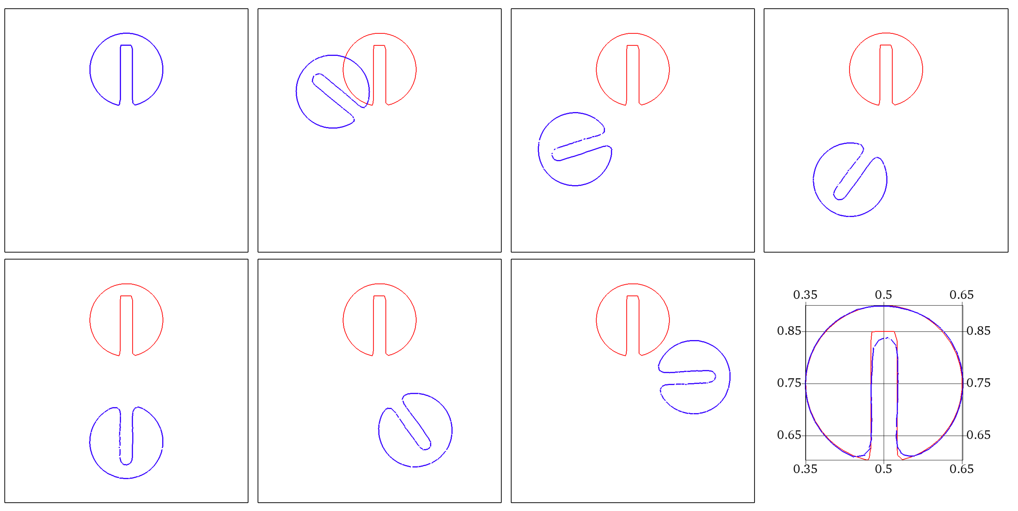
4.2. Level Set Example–Spatial Convergence

To investigate spatial accuracy, we consider the Zalesak test of a solid slotted disk in a periodic rotation. This test is commonly used to assess the performance of interface tracking methods [48]. Consider a slotted circle of radius 0.15 initially centered at ( 0.5 , 0.75 ) and having a slot of depth 1 / 4 and width 1 / 10 . The slotted circle is advected by a rotational field given by u = 1 2 ( 0.5 y ) , 1 2 ( x 0.5 ) T . The computational domain is the square [ 0 , 1 ] 2 . Successive snapshots showing the rotating slotted disk are provided in Figure 4.
We perform a spatial convergence analysis by calculating the error in the L2 norm of the Heaviside of φ with respect to the exact solution after one period of rotation. Successively refined meshes with mesh size h are considered. Figure 5 plots the evolution of the logarithm of errors as a function of the logarithm of h, for continuous piecewise polynomial approximations of degrees k = 1 , k = 2 and k = 3 . A nonlinear fitting is done. Convergence slopes show that the error behaves approximately as O h k + 1 , where k is the Lagrange polynomial’s degree.

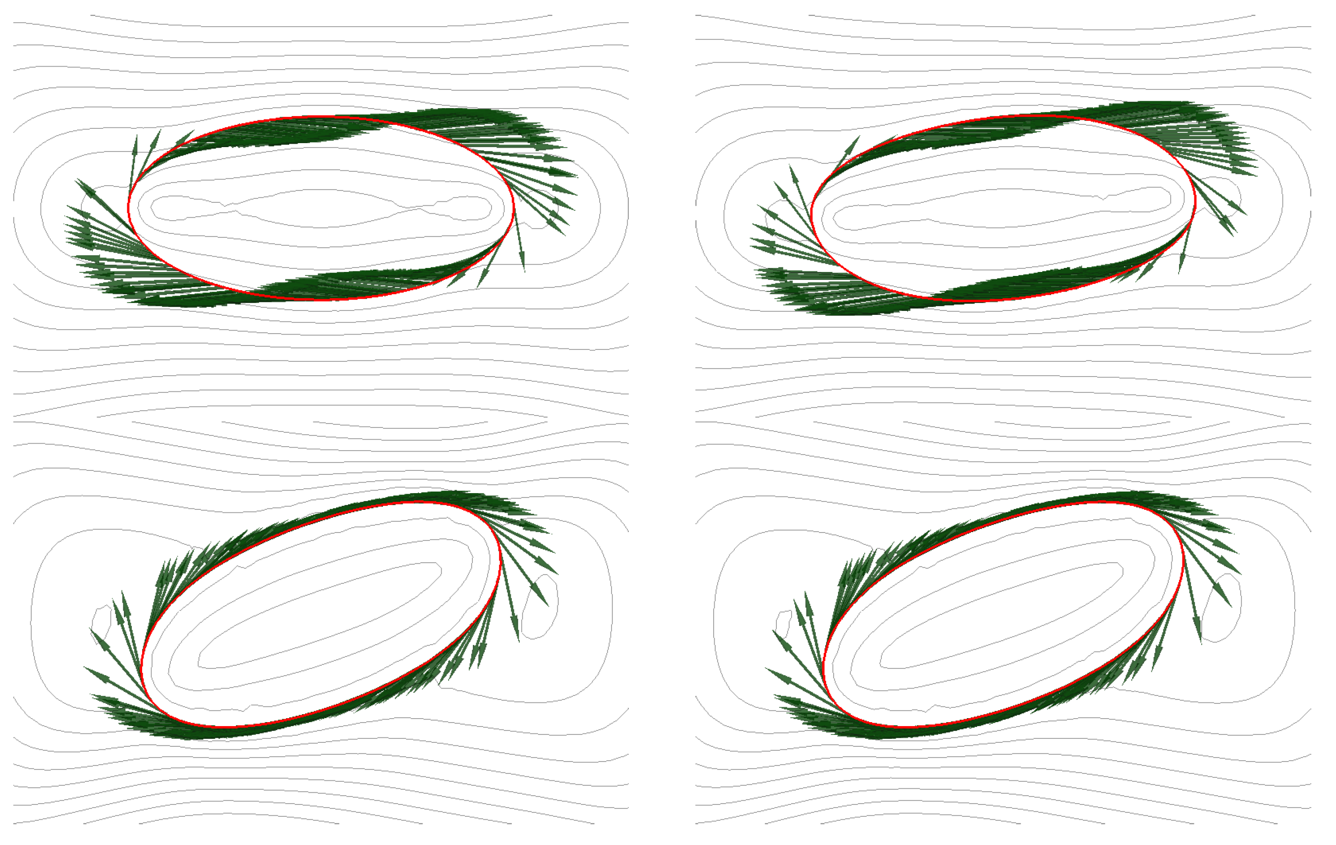
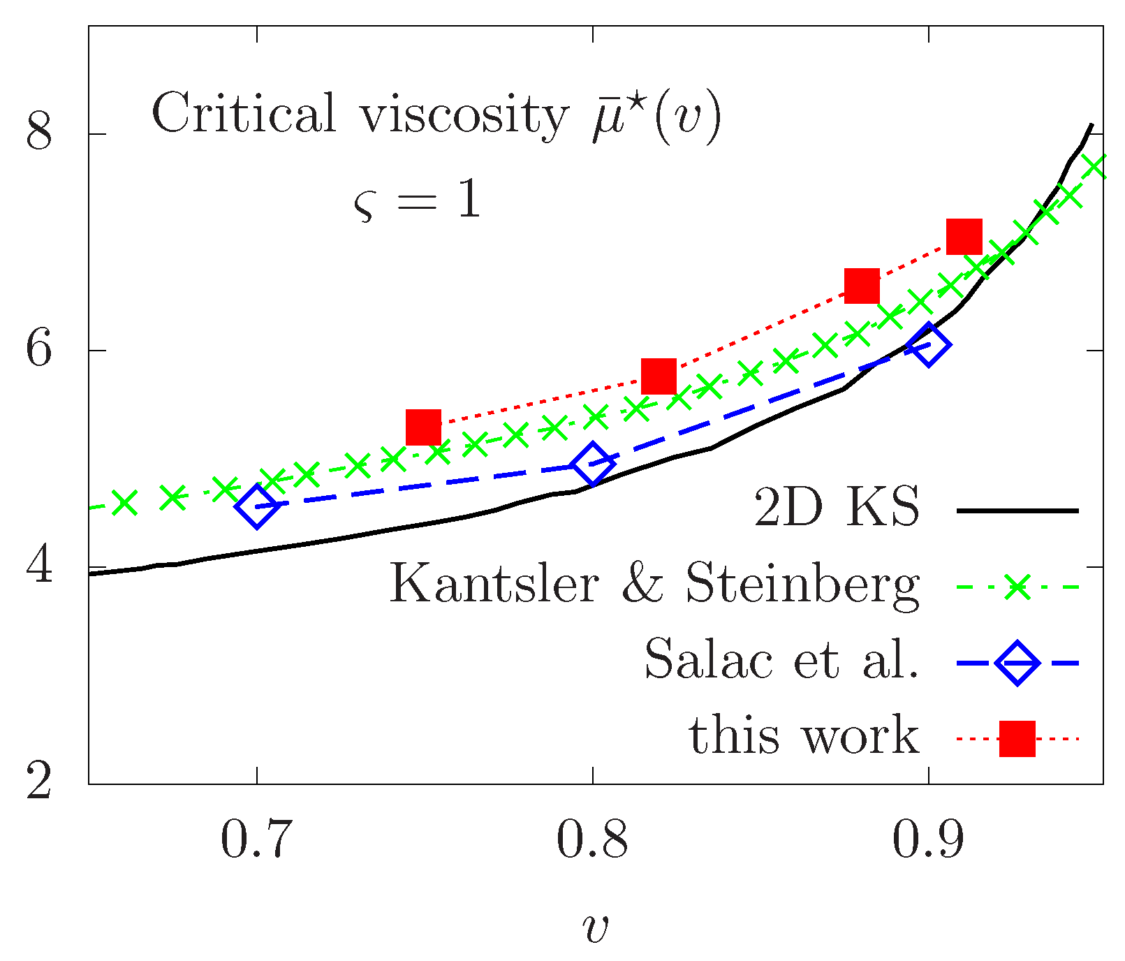
4.3. Vesicle in Linear Shear Flow

Consider a vesicle with a reduced area v = 0.77 in a simple linear shear flow and set the physical parameters to R e = 10 3 , Bn = 10 3 and ς = 0.479 . In light of the experimental observations and analysis [49], RBCs can undergo mainly two different motions, referred to as tank-treading (TT) and tumbling (TB) motions.
We first set a viscosity ratio μ ¯ = 1 and report on Figure 6 successive snapshots of the membrane dynamics in flow. Observe that the membrane Γ follows a steady state TT regime by fixing its main axis at a given equilibrium inclination angle with respect to the flow. Isocontour lines are provided in Figure 6 showing the velocity field becomes tangential to the membrane in the steady state. Indeed, each material point on the membrane continues to rotate tangentially to the flow without the vesicle changing shape.
We then increase the ratio to μ ¯ = 10 , which leads to a change of regime. The membrane loses its fluidity and undergoes a solid-like cyclic rotational motion around the interior, as shown in the snapshots in Figure 7. Indeed, the TT becomes unfavorable to the benefit of the TB when the viscosity ratio is beyond a threshold value for which the twisting force due to shear can no longer be converted into TT torque of the membrane.
Figure 8 reports the TB inclination angle θ n and adapted time steps versus the time for few rotation periods. Higher values of δ t n are successfully generated when the vesicle is close to a horizontal tilt characterized by slow rotational dynamics. However, δ t n are almost ten times smaller when the membrane is in vertical position undergoing a strong action of the orthogonal shear flow which results in a faster rotation.
Thereafter, we proceed to a qualitative validation of our model compared to some experimental and numerical results available in the published literature. We first focus on the TT-TB transition in the purely Newtonian case, where some simulation results are available. We report the critical viscosity contrast μ ¯ necessary to observe a change of regime for several values of the reduced area v in the interval [ 0.7 , 1 ] . The phase diagram is reported in Figure 9, showing good quantitative agreement with the Keller and Skalak’s 2D predictive theory [50], referred to as KS, the experimental results of Kantsler & Steinberg in [51] and the numerical calculations with the level set method in a finite differences framework in [26]. Note that the KS predictive theory is obtained by assuming a fixed ellipse shape for the vesicle, while only flow orientation is permitted. This could explain the small difference between the different results and those predicted by the KS work.
Finally, we consider a vesicle following the tank-treading motion and focus on some effects of the non-Newtonian fluid model on the TT regime. For TT vesicles at equilibrium, we report in Figure 10 the change in the equilibrium inclination angle θ with respect to the reduced area parameter v. For ς = 1 corresponding to a Newtonian fluid, only a qualitative agreement is observed with the experimental results in [51] and the numerical calculations in [12], with angles slightly shifted upwards. While the proposed penalty method features a smaller system of equations to solve, the small difference observed with respect to the numerical results obtained in [12,33] may be due to relaxation of the inextensibility instead of using an exact Lagrange multiplier [18,33] imposing this constraint.
We now study the equilibrium inclination angle of tank-treading vesicles immersed in a non-Newtonian Carreau fluid. Simulation results are also reported in Figure 10, illustrating lower values of the equilibrium angle θ are obtained, for various reduced area parameters. Our interpretation is as follows. At the vesicle scale in small capillaries, the length scale and velocity are typically around 10 μ m and 1–100 μ m / s , respectively. The local shear rate is of the order of 0.1–10 < 100 s 1 (typical value characterizing the transition to a Newtonian behavior), resulting in an apparent viscosity closer to the infinite-shear viscosity. As a consequence, the fluid is much denser and tends to decrease the inclination angle at equilibrium.

5. Conclusions

We have presented a numerical method for the simulation of the dynamics of a single vesicle in non-Newtonian flow. The membrane is described by a level set function, while the inextensibility is relaxed by a penalty method. The penalty method is straightforward to implement using any Stokes solver generally available in finite element libraries and features a smaller system of equations to solve. The order of the temporal scheme is raised according to the double composition of the numerical flow associated with the first-order backward Euler integrator. Moreover, an adaptive time-stepping strategy is based on an error estimation and allows to improve the prediction of the membrane dynamics. The numerical results show that we are able to accurately reproduce the cellular regimes under linear shear flow as well as the regime change from tank-treading to tumbling in the Newtonian case. Last but not least, a change of regime due to a non-Newtonian rheology is highlighted.
The non-Newtonian effect will be further explored in a separate work, in the hope of prompting experiments to explore it in depth. This is part of a larger study of the dynamics of 3D biological membrane and RBCs with hyperelastic cytoskeleton in non-Newtonian flows [25,52]. This requires the development of a robust solver for fluid–structure interaction problems with a thin elastic structure [53,54]. Other extensions of the presented method are being currently explored. We are particularly focusing on the development of higher-order schemes by multi-step composition of various basic integrators. The construction of robust preconditioners is also being explored.

Funding

The author gratefully acknowledges the financial support by KUST through the grant FSU-2021-027 (#8474000367).

Data Availability Statement

Not applicable.

Conflicts of Interest

The author declares no conflict of interest.

References

  1. Noyhouzer, T.; L’Homme, C.; Beaulieu, I.; Mazurkiewicz, S.; Kuss, S.; Kraatz, H.B.; Canesi, S.; Mauzeroll, J. Ferrocene-Modified Phospholipid: An Innovative Precursor for Redox-Triggered Drug Delivery Vesicles Selective to Cancer Cells. Langmuir 2016, 32, 4169–4178. [Google Scholar] [CrossRef]
  2. Ayscough, S.E.; Clifton, L.A.; Skoda, M.W.; Titmuss, S. Suspended phospholipid bilayers: A new biological membrane mimetic. J. Colloid Interface Sci. 2023, 633, 1002–1011. [Google Scholar] [CrossRef] [PubMed]
  3. Karaz, S.; Senses, E. Liposomes Under Shear: Structure, Dynamics, and Drug Delivery Applications. Adv. NanoBiomed Res. 2023; in press. [Google Scholar] [CrossRef]
  4. Kwon, O.; Krishnamoorthy, M.; Cho, Y.I.; Sankovic, J.M.; Banerjee, R.K. Effect of Blood Viscosity on Oxygen Transport in Residual Stenosed Artery Following Angioplasty. J. Biomech. Eng. 2008, 130, 011003. [Google Scholar] [CrossRef] [PubMed]
  5. P, P.C.; Simmonds, M.; Brun, J.; Baskurt, O. Exercise hemorheology: Classical data, recent findings and unresolved issues. Clin. Hemorheol. Microcirc. 2013, 53, 187–199. [Google Scholar] [CrossRef]
  6. Wajihah, S.A.; Sankar, D. A review on non-Newtonian fluid models for multi-layered blood rheology in constricted arteries. Arch. Appl. Mech. 2023, 1–26. [Google Scholar] [CrossRef]
  7. Chien, S.; Usami, S.; Dellenback, R.; Gregersen, M. Shear-dependent deformation of erythrocytes in rheology of human blood. Am. J. Physiol. 1970, 219, 136–142. [Google Scholar] [CrossRef]
  8. Lai, M.C.; Li, Z. A remark on jump conditions for the three-dimensional Navier–Stokes equations involving an immersed moving membrane. Appl. Math. Lett. 2001, 14, 149–154. [Google Scholar] [CrossRef]
  9. Pozrikidis, C. Numerical simulation of the flow-induced deformation of red blood cells. Ann. Biomed. Eng. 2003, 31, 1194–1205. [Google Scholar] [CrossRef]
  10. Rahimian, A.; Veerapaneni, S.K.; Biros, G. Dynamic simulation of locally inextensible vesicles suspended in an arbitrary two-dimensional domain, a boundary integral method. J. Comput. Phys. 2010, 229, 6466–6484. [Google Scholar] [CrossRef]
  11. Boedec, G.; Leonetti, M.; Jaeger, M. 3D vesicle dynamics simulations with a linearly triangulated surface. J. Comput. Phys. 2011, 230, 1020–1034. [Google Scholar] [CrossRef]
  12. Seol, Y.; Tseng, Y.H.; Kim, Y.; Lai, M.C. An immersed boundary method for simulating Newtonian vesicles in viscoelastic fluid. J. Comput. Phys. 2019, 376, 1009–1027. [Google Scholar] [CrossRef]
  13. Krüger, T.; Varnik, F.; Raabe, D. Efficient and accurate simulations of deformable particles immersed in a fluid using a combined immersed boundary lattice Boltzmann finite element method. Comput. Math. Appl. 2011, 61, 3485–3505. [Google Scholar] [CrossRef]
  14. Kaoui, B.; Harting, J.; Misbah, C. Two-dimensional vesicle dynamics under shear flow: Effect of confinement. Phys. Rev. E 2011, 83, 066319. [Google Scholar] [CrossRef]
  15. Bonito, A.; Nochetto, R.H.; Pauletti, M.S. Parametric FEM for geometric biomembranes. J. Comput. Phys. 2010, 229, 3171–3188. [Google Scholar] [CrossRef]
  16. Barrett, J.W.; Garcke, H.; Nurnberg, R. Numerical computations of the dynamics of fluidic membranes and vesicles. Phys. Rev. E 2015, 92, 052704. [Google Scholar] [CrossRef] [PubMed]
  17. Cottet, G.H.; Maitre, E.; Milcent, T. Eulerian formulation and Level-Set models for incompressible fluid–structure interaction. Math. Model. Numer. Anal. 2008, 42, 471–492. [Google Scholar] [CrossRef]
  18. Laadhari, A.; Saramito, P.; Misbah, C. Computing the dynamics of biomembranes by combining conservative level set and adaptive finite element methods. J. Comput. Phys. 2014, 263, 328–352. [Google Scholar] [CrossRef]
  19. Doyeux, V.; Guyot, Y.; Chabannes, V.; Prud’homme, C.; Ismail, M. Simulation of two-fluid flows using a finite element/level set method. Application to bubbles and vesicle dynamics. J. Comput. Appl. Math. 2013, 246, 251–259. [Google Scholar] [CrossRef]
  20. Ismail, M.; Lefebvre-Lepot, A. A necklace model for vesicles simulations in 2D. Int. J. Numer. Meth. Fluids. 2014, 76, 835–854. [Google Scholar] [CrossRef]
  21. Zhang, T.; Wolgemuth, C.W. A general computational framework for the dynamics of single- and multi-phase vesicles and membranes. J. Comput. Phys. 2022, 450, 110815. [Google Scholar] [CrossRef] [PubMed]
  22. Du, Q.; Liu, C.; Wang, X. A phase field approach in the numerical study of the elastic bending energy for vesicle membranes. J. Comput. Phys. 2004, 198, 450–468. [Google Scholar] [CrossRef]
  23. Jamet, D.; Misbah, C. Toward a thermodynamically consistent picture of the phase-field model of vesicles: Curvature energy. Phys. Rev. E 2008, 78, 031902. [Google Scholar] [CrossRef] [PubMed]
  24. Valizadeh, N.; Rabczuk, T. Isogeometric analysis of hydrodynamics of vesicles using a monolithic phase-field approach. Comput. Methods Appl. Mech. Eng. 2022, 388, 114191. [Google Scholar] [CrossRef]
  25. Gera, P.; Salac, D. Modeling of multicomponent three-dimensional vesicles. Comput. Fluids 2018, 172, 362–383. [Google Scholar] [CrossRef]
  26. Salac, D.; Miksis, M. Reynolds number effects on lipid vesicles. J. Fluid Mech. 2012, 711, 122–146. [Google Scholar] [CrossRef]
  27. Canham, P. The minimum energy of bending as a possible explanation of the biconcave shape of the human red blood cell. J. Theor. Biol. 1970, 26, 61–81. [Google Scholar] [CrossRef] [PubMed]
  28. Helfrich, W. Elastic properties of lipid bilayers: Theory and possible experiments. Z. Naturforsch. C 1973, 28, 693–703. [Google Scholar] [CrossRef]
  29. Deuling, H.; Helfrich, W. The curvature elasticity of fluid membranes: A catalog of vesicle shapes. J. Phys. 1976, 37, 1335–1345. [Google Scholar] [CrossRef]
  30. Evans, E.A. Bending Resistance and Chemically Induced Moments in Membrane Bilayers. Biophys. J. 1974, 14, 923–931. [Google Scholar] [CrossRef]
  31. Barrett, J.W.; Garcke, H.; Nürnberg, R. Finite element approximation for the dynamics of fluidic two-phase biomembranes. ESAIM M2AN Math. Model. Numer. Anal. 2017, 51, 2319–2366. [Google Scholar] [CrossRef]
  32. Dziuk, G. Computational parametric Willmore flow. Numer. Math. 2008, 111, 55–80. [Google Scholar] [CrossRef]
  33. Laadhari, A.; Saramito, P.; Misbah, C.; Székely, G. Fully implicit methodology for the dynamics of biomembranes and capillary interfaces by combining the Level Set and Newton methods. J. Comput. Phys. 2017, 343, 271–299. [Google Scholar] [CrossRef]
  34. Osher, S.; Sethian, J.A. Front propaging with curvature deppend speed: Agorithms based on Hamilton-Jacobi formulations. J. Comput. Phys. 1988, 79, 12–49. [Google Scholar] [CrossRef]
  35. Laadhari, A.; Székely, G. Eulerian finite element method for the numerical modeling of fluid dynamics of natural and pathological aortic valves. J. Comput. Appl. Math. 2016, 319, 236–261. [Google Scholar] [CrossRef]
  36. Laadhari, A. Exact Newton method with third-order convergence to model the dynamics of bubbles in incompressible flow. Appl. Math. Lett. 2017, 69, 138–145. [Google Scholar] [CrossRef]
  37. Laadhari, A.; Szekely, G. Fully implicit finite element method for the modeling of free surface flows with surface tension effect. Int. J. Numer. Methods Eng. 2017, 111, 1047–1074. [Google Scholar] [CrossRef]
  38. Saramito, P. Complex Fluid Modelling and Algorithms, 1st ed.; Springer International Publishing: Cham, Switzerland, 2016; p. 302. ISBN 9783319443614. [Google Scholar] [CrossRef]
  39. Walter, J.; Salsac, A.V.; Barthes-Biesel, D. Ellipsoidal capsules in simple shear flow. J. Fluid Mech. 2011, 676, 318–347. [Google Scholar] [CrossRef]
  40. Zhang, T.; Wolgemuth, C.W. Sixth-Order Accurate Schemes for Reinitialization and Extrapolation in the Level Set Framework. J. Sci. Comput. 2020, 83, 1–21. [Google Scholar] [CrossRef]
  41. Beaucourt, J.; Rioual, F.; Séon, T.; Biben, T.; Misbah, C. Steady to unsteady dynamics of a vesicle in a flow. Phys. Rev. E 2004, 69, 011906. [Google Scholar] [CrossRef] [PubMed]
  42. Laadhari, A. Implicit finite element methodology for the numerical modeling of incompressible two-fluid flows with moving hyperelastic interface. Appl. Math. Comput 2018, 333, 376–400. [Google Scholar] [CrossRef]
  43. Janela, J.; Lefebvre, A.; Maury, B. A penalty method for the simulation of fluid–Rigid body interaction. ESAIM Proc. 2005, 14, 115–123. [Google Scholar] [CrossRef]
  44. Hairer, E.; Lubich, C.; Wanner, G. Geometric Numerical Integration: Structure-Preserving Algorithms for Ordinary Differential Equations, 2nd ed.; Springer Series in Computational Mathematics; Springer: Berlin/Heidelberg, Germany, 2002. [Google Scholar]
  45. Casas, F.; Chartier, P.; Escorihuela-Tomas, A.; Zhang, Y. Compositions of pseudo-symmetric integrators with complex coefficients for the numerical integration of differential equations. J. Comput. Appl. Math. 2021, 381, 113006. [Google Scholar] [CrossRef]
  46. Guo, S.; Ren, J. A novel adaptive Crank-Nicolson-type scheme for the time fractional Allen-Cahn model. Appl. Math. Lett. 2022, 129, 107943. [Google Scholar] [CrossRef]
  47. Saramito, P. Efficient C++ Finite Element Computing with Rheolef, CNRS-CCSD ed.; Grenoble, France. 2020, p. 259. HAL version: V15. Available online: https://cel.hal.science/cel-00573970v16 (accessed on 26 September 2022).
  48. Zalesak, S.T. Fully multidimensional flux-corrected transport algorithms for fluids. J. Comput. Phys. 1979, 31, 335–362. [Google Scholar] [CrossRef]
  49. Fischer, T.M.; Stöhr-Liesen, M.; Schmid-Schönbein, H. The Red Cell as a Fluid Droplet: Tank Tread-Like Motion of the Human Erythrocyte Membrane in Shear Flow. Science 1978, 202, 894–896. [Google Scholar] [CrossRef] [PubMed]
  50. Keller, S.R.; Skalak, R. Motion of a tank-treading ellipsoidal particle in a shear flow. J. Fluid Mech. 1982, 120, 27–47. [Google Scholar] [CrossRef]
  51. Kantsler, V.; Steinberg, V. Transition to Tumbling and Two Regimes of Tumbling Motion of a Vesicle in Shear Flow. Phys. Rev. Lett. 2006, 96, 036001. [Google Scholar] [CrossRef] [PubMed]
  52. Laadhari, A.; Barral, Y.; Székely, G. A data-driven optimal control method for endoplasmic reticulum membrane compartmentalization in budding yeast cells. Math. Methods Appl. Sci. 2023, 1. [Google Scholar] [CrossRef]
  53. Laadhari, A. An operator splitting strategy for fluid–structure interaction problems with thin elastic structures in an incompressible Newtonian flow. Appl. Math. Lett. 2018, 81, 35–43. [Google Scholar] [CrossRef]
  54. Gizzi, A.; Ruiz-Baier, R.; Rossi, S.; Laadhari, A.; Cherubini, C.; Filippi, S. A three-dimensional continuum model of active contraction in single cardiomyocytes. Model. Simul. Appl. 2015, 14, 157–176. [Google Scholar] [CrossRef]
Figure 1. Representation of a vesicle Γ immersed a computational domain Λ under simple shear flow conditions.
Mathematics 11 01950 g001
Figure 2. Temporal convergence for different time schemes as a function of constant time steps δ t .
Mathematics 11 01950 g002
Figure 3. Comparative study of the accuracy between the solutions obtained using different adaptation strategies versus a constant time step. Time evolution of the adapted time step (a), error (b) and computed solution (c).
Mathematics 11 01950 g003
Figure 4. Spatial convergence in the L2 norm for the rotating Zalesak disk as a function of the mesh size h.
Mathematics 11 01950 g004
Figure 5. Zalesak test case. Snapshots showing the rotation of the slotted disk at successive times t = 0 , 1.76 , 3.77 , 5.03 , 2.28 , 7.54 , 9.55 , 4 π . The shape (blue color) obtained is compared to the exact solution after a complete rotation period (red color).
Mathematics 11 01950 g005
Figure 6. Vesicle with reduced area v = 0.77 following a TT regime in simple shear flow at times t { 0.01 , 0.14 , 0.52 , 1.6 } . Dimensionless parameters: μ ¯ = 1 , Re = 10 3 and Bn = 10 3 . The membrane is plotted in red, while the tangential velocity is plotted in green. [Colour figure can be viewed online].
Mathematics 11 01950 g006
Figure 7. Flowing vesicle with v = 0.77 following a TB regime for μ ¯ = 10 , Re = 10 3 and Bn = 10 3 at times t { 2.27 , 2.70 , 2.88 , 3.09 , 3.25 , 3.62 } . The membrane is plotted in red, while the tangential velocity is plotted in green. [Colour figure can be viewed online].
Mathematics 11 01950 g007
Figure 8. Flowing vesicle under TB regime: Adapted time steps δ t n and inclination angle θ n for a vesicle in a tumbling regime.
Mathematics 11 01950 g008
Figure 9. Phase diagram of the TT-TB transition versus the reduced area v in the Newtonian case. Comparison with 2D KS theory [50], experimental results of Kantsler & Steinberg in [51] and numerical computations in [26]. [Colour figure can be viewed online].
Mathematics 11 01950 g009
Figure 10. Vesicle in the TT regime. Equilibrium inclination angle θ versus different reduced areas v. Comparison with the experiments in [51] and numerical results in [12,33].
Mathematics 11 01950 g010
Disclaimer/Publisher’s Note: The statements, opinions and data contained in all publications are solely those of the individual author(s) and contributor(s) and not of MDPI and/or the editor(s). MDPI and/or the editor(s) disclaim responsibility for any injury to people or property resulting from any ideas, methods, instructions or products referred to in the content.

