Parametric Study on the Sensitivity of Different Properties of Waves Propagating through an Incompressible Medium

Abstract

This article deals with the study of disturbance that travels through the transversely isotropic medium in the form of waves. The particles of the considered medium have an additional property of small-scale internal rotation along with macroscopic translational deformation. This extra translational freedom causes the medium to be micropolar in nature. Along with this, the medium is incompressible, and the dispersion relation of waves propagating through the medium is obtained under specific plan-strain conditions. From the dispersion relation, we can conclude that because of incompressibility, three transverse waves propagate through the medium. The velocity profile, attenuation coefficient, and specific heat loss for these waves are discussed for a particular medium. Later, the special normalized local sensitivity analysis (NLSA) technique is used to depict the effects of parameters on the outcomes of the mathematical model. The obtained results are represented graphically for a particular medium. The proposed model is used to model the mechanical behavior of complex materials with microstructural heterogeneity, such as composites and biological tissues.

1. Introduction

The theory of elasticity is a branch of solid mechanics that deals with the deformation and stress of solid materials under applied loads. It provides mathematical equations to describe the behavior of materials under different types of loading, such as tension, compression, bending, and torsion. It also provides solutions for the calculation of stresses, strains, and displacements in solid structures. The applications of the theory of elasticity are numerous and include the design and analysis of structures such as bridges, buildings, and aircraft, as well as the study of the mechanical behavior of materials such as metals, polymers, and composites. It is also used in fields such as geomechanics, biomechanics, and acoustics.

The theory of elasticity also deals with the propagation of waves through an elastic media under certain conditions. In general, in an isotropic medium, only two waves propagate; longitudinal and transverse. In a transversely isotropic medium with three waves, one wave is quasi-longitudinal, and two quasi-transverse waves propagate [1]. The condition of incompressibility restricts the existence of longitudinal waves, resulting in the generation of only two transverse waves [2]. Because of the micropolar theory of elasticity, the symmetry of stress and a strain tensor does not exist, which allows another wave to propagate in the medium. Singh [3] discussed the problem of wave propagation in an incompressible transversely isotropic fiber-reinforced elastic medium and obtained the reflection coefficients for the case of the outer slowness section. The work was extended by many authors and introduced the concept of initial stresses along with incompressibility [4,5,6].

The linear theory of micropolar thermoelasticity was introduced by Eringen [7], and the waves through such types of materials are done by Smith [8]. The reflection phenomena of waves through a flat boundary of a micropolar elastic half-space medium were studied by Parfitt and Eringen [9]. The concept of a fiber-reinforced micropolar medium was studied for surface waves by Sengupta and Nath [10]. Elastic waves in a fiber-reinforced medium were also studied by Bose and Mal [11]. Recently, several researchers used the literature study of a fiber-reinforced medium and analyzed the different types of surface waves propagating through the medium [12,13,14,15,16,17,18].

In this article, we have studied the propagation of waves with constant amplitude propagating through a thermoelastic medium. The medium considered is transversely isotropic, with the additional properties of micro-rotational deformation and incompressibility. The mathematical model for the said medium is formulated to obtain the dispersion relation of the harmonic waves propagating through the medium. It is found that because of incompressibility, three transverse waves propagate through a micropolar fiber-reinforced transversely isotropic medium. A technique of normalized local sensitivity analysis is used to depict the effects of the parameters on the outcomes of the mathematical model. The study is useful in different branches of engineering, such as Bioinformatics, Seismic retrofitting, and specifically civil engineering, where there is a need for high-strength materials that also maintain a low weight.

2. Basic Constitutive Relations

It is also important to mention that any second-rank tensor can be expressed as the sum of symmetric and anti-symmetric tensors as

$${\theta }_{ij}=\frac{1}{2}\left({\theta }_{ij}+{\theta }_{ji}\right)+\frac{1}{2}\left({\theta }_{ij}-{\theta }_{ji}\right),$$

$${\theta }_{ij}={\theta }_{ij}^s+{\theta }_{ij}^a.$$

On applying the same condition, the strain tensor can be rephrased as

$$\mathrm{\Xi }={\mathrm{\Xi }}^{\mathrm{s}}+{\mathrm{\Xi }}^{\mathrm{a}},$$

where $\mathrm{\Xi }=\left[e_{ij},{\sigma }_{ij},m_{ij}\right]$ presents the strain, stress, and coupled stress for the micropolar thermoelastic medium. The total strain tensor for the micropolar theory of linear thermoelasticity is given by the following relations [2,3]:

$$e_{ij}=u_{j,i}-{ϵ}_{ijk}{\varphi }_k,$$

where $u$ is the displacement field vector, $\varphi$ is the microrotational vector field for the micropolar medium.

The classical constitutive relation for an incompressible transversely isotropic fiber-reinforced medium, considered by Rogerson [2] and Singh [3], can be written as follows:

$${\sigma }_{ij}=-P{\delta }_{ij}+2\mu e_{ij}+2\left({\mu }_L-{\mu }_T\right)\left({\delta }_{i1}{e}_{j1}-{\delta }_{j1}{e}_{j1}\right)+4\left({\mu }_E-{\mu }_L\right)e_{11}{\delta }_{i1}{\delta }_{j1},$$

where ${\mu }^{\prime }s$ are material constants and $e_{ij}=\frac{u_{i,j}+u_{j,i} }{2}$. An incompressible transversely isotropic medium has three degrees of freedom, whereas a micropolar medium has 6 degrees of freedom. The stress tensor and coupled stress tensor are not symmetric in a micropolar medium. The relation for stresses for a micropolar medium with a fiber-reinforced structure can be represented as

$$\begin{array}{c}{\sigma }_{ij}=-P{\delta }_{ij}+2\left({\mu }_{L1}-{\mu }_{T1}\right)\left\{{\delta }_{j1}\left(e_{i1}-e_{1i}\right)+{\delta }_{i1}\left(e_{j1}+e_{1j}\right)\right\}\left({\mu }_{L1}+{\mu }_{T2}\right)\\ \hspace{1em}\hspace{1em}\hspace{1em}\hspace{1em}\hspace{1em}\hspace{1em}+\left({\mu }_{T1}+{\mu }_{T2}\right)e_{ij}+\left({\mu }_{T1}-{\mu }_{T2}\right)e_{ji}\\ \hspace{1em}\hspace{1em}\hspace{1em}\hspace{1em}\hspace{1em}\hspace{1em}+\left({\mu }_{L2}-{\mu }_{T2}\right)e_{ij}\left\{{\delta }_{i1}\left(e_{j1}-e_{1j}\right)+{\delta }_{j1}\left(e_{i1}-e_{1i}\right)\right\}\\ \hspace{1em}\hspace{1em}\hspace{1em}\hspace{1em}\hspace{1em}\hspace{1em}+4\left({\mu }_{E1}-{\mu }_{L1}\right)e_{11}{\delta }_{i1}{\delta }_{j1},\end{array}$$

$$\begin{array}{c}{m}_{ij}=-P{\delta }_{ij}+\left({\lambda }_{L1}-{\lambda }_{T1}\right)\left\{{\delta }_{j1}\left({\mathrm{\chi }}_{i1}-{\mathrm{\chi }}_{1i}\right)+{\delta }_{i1}\left({\mathrm{\chi }}_{j1}+{\mathrm{\chi }}_{1j}\right)\right\}+\left({\lambda }_{T1}+{\lambda }_{T2}\right){\mathrm{\chi }}_{ij}\\ \hspace{1em}\hspace{1em}\hspace{1em}\hspace{1em}\hspace{1em}\hspace{1em}+\left({\lambda }_{T1}-{\mu }_{T2}\right){\mathrm{\chi }}_{ji}\\ \hspace{1em}\hspace{1em}\hspace{1em}\hspace{1em}\hspace{1em}\hspace{1em}+\left({\mu }_{L2}-{\mu }_{T2}\right){\mathrm{\chi }}_{ji}\left\{{\delta }_{i1}\left(e_{j1}-e_{1j}\right)+{\delta }_{j1}\left(e_{i1}-e_{1i}\right)\right\}\\ \hspace{1em}\hspace{1em}\hspace{1em}\hspace{1em}\hspace{1em}\hspace{1em}+4\left({\mu }_{E1}-{\mu }_{L1}\right)e_{11}{\delta }_{i1}{\delta }_{j1},\end{array}$$

where ${\sigma }_{ij}^a,{\sigma }_{ij}^s,m_{ij}^a \mathrm{and}{m}_{ij}^s$ are represented in Appendix A. By using the above-derived relation, the balance laws for the selected medium are represented by the following relations:

$${\sigma }_{ji,j}=\rho {\ddot{u}}_i,$$

(1)

$$m_{ji,j}+{ϵ}_{imn}{\sigma }_{mn}=\rho J{\ddot{\varphi }}_i,$$

(2)

where J is micro-inertia, $\mathrm{and} m_{ij}$, ${\sigma }_{ij}$, $u_i, \rho$ and ${\varphi }_i$ are the couple stress tensor, stress tensor, displacement vector, mass density, and micro-rotation vector, respectively.

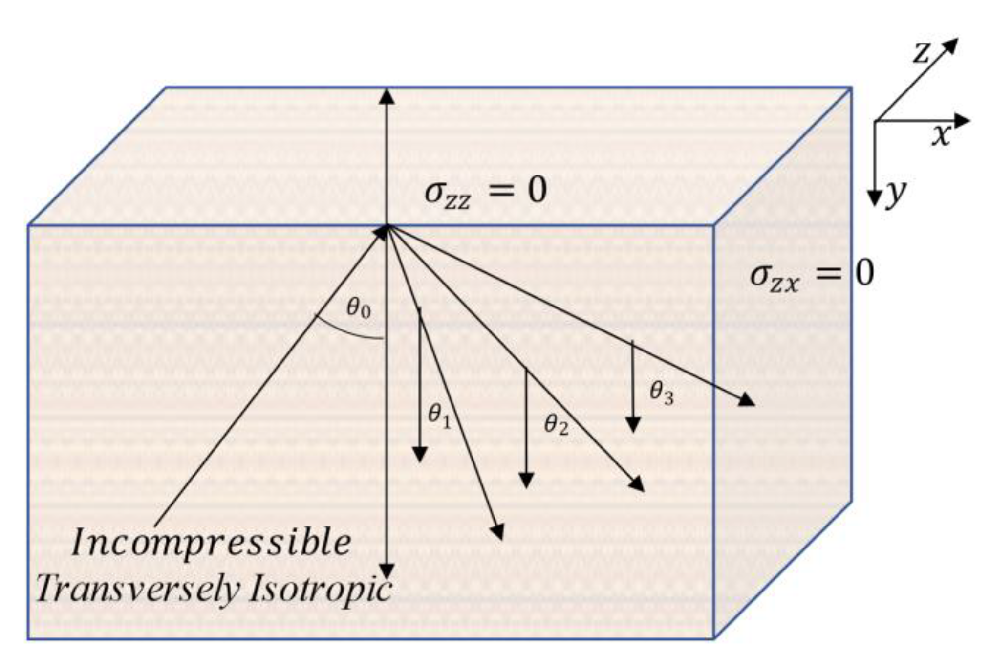
3. Formulation of the Problem

We considered an incompressible micropolar transversely isotropic fiber-reinforced medium. The complexity of the problem can be reduced by considering the following plain strain problem:

$$u_i\left(x,y,z\right)=\left(u_1,u_2,0\right),{\varphi }_i\left(x,y,z\right)=\left(0,0,{\varphi }_3\right).$$

The state is initially considered to be undisturbed at a reference temperature. Then, the initial and regular conditions are as follows:

$$\left\{\begin{array}{c}{u}_i\left(x,y,0\right)=0=\dot{u_i}\left(x,y,0\right)\\ \varphi \left(x,y,0\right)=0=\dot{\varphi }\left(x,y,0\right)\end{array}\right\};z\ge 0.$$

From the essential criteria for the linearized incompressibility condition, we have

$$u_{1,1}+u_{2,2}+u_{3,3}=0 or u_{i,i}=0.$$

The last equation shows that the polarization vector and propagation vector are mutually perpendicular, which is true for transverse waves. Hence, only transverse waves propagate in an incompressible medium.

Using the above-mentioned supposition along with the incompressibility condition, the wave equation of motion (1) can be represented as

$$\begin{array}{c}-P_i+\left({\mu }_{T1}+{\mu }_{T2}\right)e_{ji,j}+\left({\mu }_{T1}-{\mu }_{T2}\right)e_{ij,j}\\ \hspace{1em}\hspace{1em}\hspace{1em}\hspace{1em}\hspace{1em}\hspace{1em}+\left({\mu }_{L1}+{\mu }_{T2}\right)\left\{{\delta }_{j1}\left(e_{i1,j}+e_{1i,j}\right)+{\delta }_{i1}\left(e_{j1,j}+e_{1j,j}\right)\right\}\\ \hspace{1em}\hspace{1em}\hspace{1em}\hspace{1em}\hspace{1em}\hspace{1em}+\left({\mu }_{L2}-{\mu }_{T2}\right)\left\{{\delta }_{j1}\left(e_{i1,j}-e_{1i,j}\right)+{\delta }_{i1}\left(e_{j1,j}-e_{1j,j}\right)\right\}\\ \hspace{1em}\hspace{1em}\hspace{1em}\hspace{1em}\hspace{1em}\hspace{1em}+4\left({\mu }_{E1}-{\mu }_{L1}\right)e_{11,j}{\delta }_{i1}{\delta }_{j1}=\rho {\ddot{u}}_i\end{array}$$

(3)

Here, $P$ is the pressure to maintain the incompressible condition, and ${\mu }_{T1},{\mu }_{T2},{\mu }_{L1},{\mu }_{L2},$ ${\lambda }_{T1},{\lambda }_{T2},{\lambda }_{L1}$ and ${\lambda }_{L2}$ are the elastic constants of the material.

$${\mu }_E=\frac{E_{L1}}{E_{T1}}{\mu }_{T1}, {\lambda }_E=\frac{E_{L2}}{E_{T2}}{\lambda }_{T1},$$

In above relation, $E_{L1}$, $E_{L2}$ and $E_{T1}$, $E_{T2}$ are longitudinal transverse Young’s moduli, respectively.

4. Propagation of Wave in the Medium

We take the two-dimensional motion of the wave in a micropolar incompressible transversely isotropic fiber-reinforced half space $\left\{x, y\ge 0\right\}.$ There is a plane shear wave with constant amplitude moving along the surface, with a polarization vector $n_i,$ with some angle of incidence. The proposed solution can be taken as

$$\left(u_i,{\varphi }_3,P\right)=\left(A{p}_i,k{\varphi }_0,k{P}^{*}\right)e^{i\left(k{x}_j{n}_j-\omega t\right)},$$

(4)

where $\omega =ϵ+i\upsilon$ represents the complex angular frequency, the real part is associated with an oscillation frequency of the wave, while the imaginary part represents the phase information along with the attenuation factor. The complex angular frequency is used in the study of quantum mechanics, where it describes the behavior of the particle. The polarization vector is $n_i=\left(n_1,n_2,0\right)=\left(sin\theta ,cos\theta ,0\right)$, where $\theta$ is the angle of the incident wave to the surface. By using the relation (4) system of governing, equations can be represented as

$$\begin{array}{c}-i{n}_i{k}^2{P}^{*}+\left[\rho {\omega }^2-\left({\mu }_{L1}-{\mu }_{L2}+2{\mu }_{T2}\right)k^2{n}_1^2-\left({\mu }_{T1}+{\mu }_{T2}\right)k^2{n}_2^2\right]A{p}_i\\ \hspace{1em}\hspace{1em}\hspace{1em}\hspace{1em}\hspace{1em}\hspace{1em}-\left[\left({\mu }_{L1}+{\mu }_{L2}-{\mu }_{T1}-{\mu }_{T2}\right)n_1{p}_1\right]k^{2}A{n}_i\\ \hspace{1em}\hspace{1em}\hspace{1em}\hspace{1em}\hspace{1em}\hspace{1em}+i{\varphi }_0\left[4{\mu }_{T2}-{\mu }_{L2}\right]n_1{k}^2{\epsilon }_{1i3}+i{\varphi }_0\left(2{\mu }_{T2}\right)n_2{k}^2{\epsilon }_{2i3}\\ \hspace{1em}\hspace{1em}\hspace{1em}\hspace{1em}\hspace{1em}\hspace{1em}-[\left\{\left(4{\mu }_E-2{\mu }_{L1}-2{\mu }_{T1}\right)n_1^2+\left({\mu }_{L1}+{\mu }_{L2}-{\mu }_{T1}-{\mu }_{T2}\right)n_2^2\right\}A{p}_1\\ \hspace{1em}\hspace{1em}\hspace{1em}\hspace{1em}\hspace{1em}\hspace{1em}+\left\{\left({\mu }_{L1}-{\mu }_{L2}+{\mu }_{T2}-{\mu }_{T1}\right)n_1{n}_2\right\}A{p}_2\\ \hspace{1em}\hspace{1em}\hspace{1em}\hspace{1em}\hspace{1em}\hspace{1em}+2i\left({\mu }_{L2}-{\mu }_{T2}\right){\varphi }_0{n}_2]k^2{\delta }_{i1}=0,\end{array}$$

(5)

$$\begin{array}{c}\left(-2ik{\mu }_{T2}{n}_2\right)A{p}_1+\left(2ik{\mu }_{T2}{n}_1\right)A{p}_2\\ \hspace{1em}\hspace{1em}\hspace{1em}\hspace{1em}\hspace{1em}\hspace{1em}+[k^2\left\{\rho J{w}^2-\left({\lambda }_{L1}-{\lambda }_{L2}+2{\lambda }_{T2}\right)n_1^2-\left({\lambda }_{T1}+{\lambda }_{T2}\right)n_2^2\right\}\\ \hspace{1em}\hspace{1em}\hspace{1em}\hspace{1em}\hspace{1em}\hspace{1em}+4{\mu }_{T2}]{\varphi }_0=0.\end{array}$$

(6)

Now, multiplying the Equation (5) with $n_i$ and employing the incompressibility condition $n_i{p}_i=0$ gives the following equation:

$$\begin{array}{c}{P}^{*}=i\left[\left(4{\mu }_E-2{\mu }_{L1}-{\mu }_{T1}\right)k^2{n}_1^2+\left({\mu }_{L1}+{\mu }_{L2}-{\mu }_{T1}-{\mu }_{T2}\right)\left(1+n_2^2\right)\right]k^{2}A{n}_1{p}_1\\ \hspace{1em}\hspace{1em}\hspace{1em}\hspace{1em}\hspace{1em}\hspace{1em}+i\left[\left({\mu }_{L1}-{\mu }_{L2}+{\mu }_{T2}\right)n_1^2\right]k^{2}A{n}_2{p}_2+\left[4\left({\mu }_{T2}-{\mu }_{L2}\right)n_1{n}_2{k}^2\right]{\varphi }_0\end{array}$$

(7)

The equation of motion in component form after eliminating $P^{*}$ can be written as

$$\left(\rho {\omega }^2-D_1{k}^2\right)A{p}_1+\left\{\left({\mu }_{T2}-{\beta }_1\right)k^2{n}_1{n}_3^2\right\}A{p}_2-ik{D}_3{\varphi }_0=0$$

(8)

$$\left({\beta }_5{n}_1^3{n}_2+{\beta }_3{n}_2^3{n}_1\right)k^{2}A{p}_1+\left(\rho {\omega }^2-D_2{k}^2\right)A{p}_2+ik{D}_4{\varphi }_0=0$$

(9)

$$\left(2ik{\beta }_7{n}_2\right)A{p}_1-\left(2ik{\beta }_7{n}_1\right)A{p}_2+\left(k^2{\beta }_6-4{\beta }_7-J\rho {\omega }^2\right){\varphi }_0=0$$

(10)

where the constants used in the coefficients are

$${\beta }_1=\left({\mu }_{L1}-{\mu }_{L2}+2{\mu }_{T2}\right), {\beta }_2=\left({\mu }_{T1}+{\mu }_{T2}\right), {\beta }_3=\left({\mu }_{L1}+{\mu }_{L2}-{\mu }_{T1}-{\mu }_{T2}\right),$$

$${\beta }_4=\left(4{\mu }_{T2}-2{\mu }_{L2}\right),{\beta }_5=\left(4{\mu }_{E1}-2{\mu }_{L1}-{\mu }_{T1}\right),$$

$${\beta }_6=\left({\lambda }_{L1}-{\lambda }_{L2}+2{\lambda }_{T2}\right)n_1^2+\left({\lambda }_{T1}+{\lambda }_{T2}\right)n_2^2,$$

$${\beta }_7={\mu }_{T2},D_1={\beta }_5{n}_1^2{n}_2^2+\left({\beta }_1-{\mu }_{T1}\right)n_1^2+{\beta }_3{n}_2^4-{\beta }_2{n}_2^2,$$

$$D_2={\beta }_1{n}_1^4+{\mu }_{T1}{n}_2^2,D_3=\left({\beta }_4{n}_1^4{n}_2+{\mu }_{L2}{n}_2\right),$$

$$D_4=\left(4{\beta }_7-{\beta }_4\right)\left(2n_2^2-1\right)n_1-2{\beta }_7{n}_1^3.$$

For non-trivial solutions, the determinant of coefficients of the system of Equations (8)–(10) must vanish, which implies the following third-order secular equation:

$$L_1{\left(k^2\right)}^3+L_2{\left(k^2\right)}^2+L_3\left(k^2\right)+L_4=0$$

(11)

where the secular Equation (11) is cubic in $k^2;$ hence, it will yield three roots of $k^2$. If $k_1^2$, $k_2^2$ and $k_3^2$ are the solutions of the Equation (11), then all of the six values of $k$ are of the form $k=\pm k, i=1,2,3$. Therefore, two sets of waves, containing three transverse waves each, may propagate in the medium. We are interested only in the roots with positive real parts; $k_i, i=1,2,3.$ The expressions for speed are expressed as follows. The velocities of these waves depend on the propagation vector $n_i$. The real part of the roots is producing propagation speed, while the imaginary part is causing the attenuation of the waves. We are interested in the special properties of the waves propagating through the medium. These are calculated by using the following relation:

• Velocity

The velocities of the waves can be computed as

$$V_i=\frac{\omega }{Real\left(k_i\right)}$$

• Attenuation coefficient

The attenuation coefficients are given by

$$Q_i=Img\left(k_i\right)$$

• Specific heat loss

The specific heat loss is denoted and defined as

$$S_i=4\pi \left|\frac{Img\left(k_i\right)}{Real\left(k_i\right)}\right|$$

where $V_i$, $Q_i$ and $W_i$ are the properties of each wave reflected into the medium as shown in Figure 1.

5. Normalized Sensitivity Analysis

This section deals with the special Normalized sensitivity analysis technique to study the effects of complex angular frequency $\omega =ϵ+i\upsilon$ on the properties of waves propagating through the medium. This allows a fair comparison of the relative importance of different values of real and imaginary parts of angular frequency parameters, even if they are measured in different units or have different ranges. The mathematical form of the normalized sensitivity analysis is expressed as

$$S=\frac{\partial y_i}{\partial x_j}.\frac{x_j}{y_i}$$

(12)

where $y_i$ is the $i^{\mathrm{th}}$ output variable and $x_j$ is the $j^{\mathrm{th}}$ input parameter. The Equation (12) can be solved numerically using the forward difference formula as

$$S\cong \frac{y\left(x_j+\nabla x_j\right)-y\left(x\right)}{\nabla x_j}.\frac{x_j}{y_i}$$

(13)

where $\nabla x=0.1\times x$. Local sensitivity helps to identify the critical input parameter by calculating the sensitivity of the model output to each input parameter. The local sensitivity method can help identify which input parameters have the greatest impact on the model output. This information can be used to factor further analysis and to prioritize the model. This identification of input response on output variables helps to optimize the performance of the model. It may also help with improving the accuracy of the model. Overall, the local sensitivity method is a powerful tool for analyzing the behavior of models and identifying key input parameters.

5.1. Simulation Setup

Before applying the sensitivity analysis, the most important step is to identify the input and output quantities of interest. In this paper, the input quantities of interest (QoI) are the involved parameters ($ϵ,\nu$), and the output QoI are ($c_1, c_2, c_3, Q_1, Q_2, Q_3, S_1, S_2, S_3$). Further, a 10% variation is studied for all input QoI and their effects are quantified on the output QoI using NLSA.

5.2. Algorithm to Compute NLSA

The following algorithm is used to compute sensitivity indices, $S$:

1. 

Define the model inputs and outputs (QoI):

Input QoI: =

$$ϵ,\nu$$

Output QoI: =

$$c_1, c_2, c_3, Q_1, Q_2, Q_3, S_1, S_2, S_3.$$

2. 

Evaluate the model:

Different relations for the properties of the disturbance are evaluated by increasing the parameters with nominal values. Given the nominal variation to the inputs, the model is evaluated to compute the respective outputs.

3. 

Calculation of mean absolute sensitivity:

The sensitivities are normalized by dividing them by the nominal values of the inputs. This step provides a relative measure of the sensitivity that is independent of the magnitude of the inputs. To write the sensitivity indices given in (13) in a compact way, the mean of absolute values of $S$ is calculated as

$$MA\left(S\right)=mean\left(abs\left(S\right)\right)$$

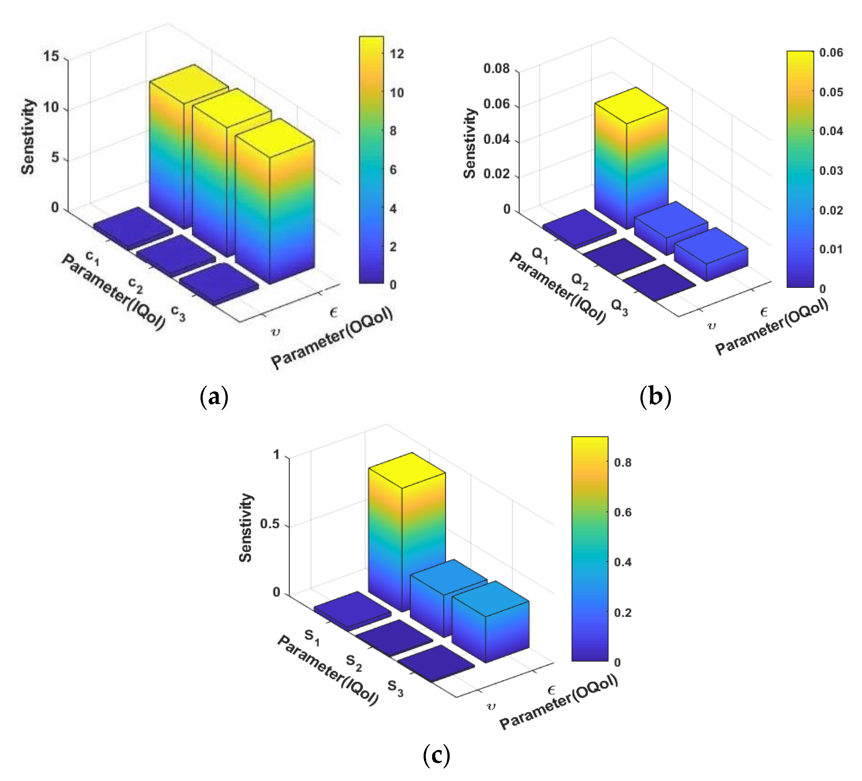
6. Results of NLSA

In this section, we will represent the findings of the NLSA method. The results will be represented for a particular medium; a carbon fiber-epoxy resin composite. It can be concluded from the graphs that different properties of the waves are more affected by the change in the parameter $ϵ$.

Figure 2 gives the three-dimensional bar view of the results obtained by using the method. It represented the response of output variables by a variating 10% increase in the input variable. From the graphical structure, we can conclude that the output parameters are highly influenced by the oscillational frequency of the wave incident in the medium. The phase information represents the position of the particle, while the wave is represented by the imaginary part of the angular frequency, and it has a comparatively small effect on the selected output variables.

7. Ranking of Important Parameters

Figure 3 gives a tabular representation of the parameters affecting the values of angular frequency. It clearly indicates that the real part of angular frequency has more effect on the properties of waves compared with the imaginary part of angular frequency. Each column in Figure 3 shows the ranking of important parameters for output. In factor fixing, we cannot fix any parameters because each parameter is sensitive to the output variables.

8. Numerical Results and Discussion

This section deals with the different properties of waves propagating through the medium, which were obtained from the Equation (11). The theoretical results obtained in the above sections are studied numerically for a particular medium, using selected elastic parameters and constants that correspond to a carbon fiber-epoxy resin composite [2].

$$\rho =7800 {\mathrm{Kgm}}^{-3}, {\mu }_{T1}=2.46\times {10}^9 {\mathrm{Nm}}^{-2},{\mu }_{T1}=2.57\times {10}^9 {\mathrm{Nm}}^{-2},$$

$${\mu }_{L1}=2.66\times {10}^9 {\mathrm{Nm}}^{-2},{\mu }_{L2}=5.23\times {10}^9 {\mathrm{Nm}}^{-2},{\lambda }_{T1}=2.66\times {10}^9 {\mathrm{Nm}}^{-2},$$

$${\lambda }_{T2}=2.32\times {10}^9 {\mathrm{Nm}}^{-2}, {\lambda }_{L1}=5.72\times {10}^9 {\mathrm{Nm}}^{-2},{\lambda }_{T2}=5.89\times {10}^9 {\mathrm{Nm}}^{-2},$$

$${\lambda }_E=59.63\times {10}^9 {\mathrm{Nm}}^{-2},{\mu }_E=59.72\times {10}^9 {\mathrm{Nm}}^{-2}.$$

In this section, we will represent a two-dimensional graphical structure for the different properties of the waves propagating through an incompressible half-space medium. The focus of the work is to study the response of the waves on the phasor frequency that is associated with the complex angular frequency $\omega =ϵ+i\upsilon$ of the wave. These types of concepts are very useful for analyzing the time-varying system, specifically used in the studies associated with electrical engineering. In the proposed solution, the real part of complex angular frequency is associated with phase velocity while the imaginary part is related to the damping factor.

Figure 4 describes the variations of the phase velocity of the three waves concerning the phasor frequency. From the graphical structure, it is found that the velocity profile of each wave propagating through the medium is directly proportional to the real part of $\nu$. However, the value of the amplitude decreases by increasing the imaginary factor of the angular frequency. For the small values of the angle of incidence, the response of the imaginary factor is the opposite. The response of phase velocity is more sensitive to the real part of the angular frequency of the incident wave.

Figure 5a–c represents the response of the attenuation factor against the angle of incidence for different values of parameters of angular frequency. The attenuation factor is responsible for the decrease in amplitude of the wave propagating through the medium. It is normally associated with the imaginary part of angular frequency. It is a very important factor of the medium, and it measures the rate at which the energy of the wave is dissipated. The first wave is directly related to the values of angular frequency, but for the second and third waves, the results are different. It can be seen from the graphical structure that the relation of the absolute value of the attenuation coefficient of the second and third waves on real and imaginary parts of angular frequency depends on the angle of incidence. For the initial values of $\theta <15°,$ it decreases by increasing both values of angular frequency, but for the values greater than this response, it is the same as that of the first wave. Further, it is noticed that the imaginary part of the angular frequency has a very small influence on the intensity of the attenuation factors. This small relation of the attenuation factor is due to complex values in the exponents and the incompressibility of the medium.

Figure 6 gives the quantitative study on the specific heat loss of waves propagating through the medium. Its intensity is directly proportional to the angle of incidence from normal to the surface. In this set of figures, we have also tried to conclude the response of specific heat loss against different values of different intensities of complex angular frequency. The real part of angular frequency has a greater impact on the specific heat loss, while the imaginary part has a small effect, comparatively.

9. Conclusions

The basic goal of this work was to study the response of different properties of generated waves to the angular frequency of the incident wave. From the secular equation, we concluded that three waves propagate through a transversely isotropic medium with fiber-reinforced properties. To study the time-varying problems in detail, we considered the angular frequency of the incident wave to be complex. The influence of both components of angular frequency is analyzed for different properties of waves. The influence of these parameters is also analyzed by the special technique of Normalized Local Sensitivity Analysis, and its effects are represented in the form of a 3D bar graph. This method also gives details about the fixing of parameters; from this analysis, we conclude that the real part of angular frequency is more influential than the imaginary part of angular frequency. We can also conclude that, in factor fixing, we cannot fix any parameter because each parameter is sensitive. This study is useful in different fields of engineering, specifically in the field of civil engineering for seismic retrofitting of structures. Using this study, we can strengthen a structure so that it becomes more resistant to earthquakes and seismic events. As a result, the study is useful for reducing the destruction caused by waves propagating through the Earth.

References

- Chadwick, P. Wave propagation in incompressible transversely isotropic elastic media I. Homogeneous plane waves. Proc. R. Ir. Acad. Sect. A Math. Phys. Sci. 1993, 93A, 231–253. [Google Scholar]
- Rogerson, G.A. Some dynamic properties of incompressible, transversely isotropic elastic media. Acta Mech. 1991, 89, 179–186. [Google Scholar] [CrossRef]
- Singh, B. Wave propagation in an incompressible transversely isotropic fibre-reinforced elastic media. Arch. Appl. Mech. 2007, 77, 253–258. [Google Scholar] [CrossRef]
- Ogden, R.; Singh, B. Propagation of waves in an incompressible transversely isotropic elastic solid with initial stress: Biot revisited. J. Mech. Mater. Struct. 2011, 6, 453–477. [Google Scholar] [CrossRef]
- Singh, B. Rayleigh Wave in an Incompressible Fibre-Reinforced Elastic Solid Half-Space. J. Solid Mech. 2016, 8, 365–371. [Google Scholar]
- Chattopadhyay, A.; Rogerson, G.A. Wave reflection in slightly compressible, finitely deformed elastic media. Arch. Appl. Mech. 2001, 71, 307–316. [Google Scholar] [CrossRef]
- Eringen, A.C. Linear theory of micropolar elasticity. J. Math. Mech. 1966, 15, 909–923. [Google Scholar]
- Smith, A.C. Waves in micropolar elastic solids. Int. J. Eng. Sci. 1967, 5, 741–746. [Google Scholar] [CrossRef]
- Parfitt, V.R.; Eringen, A.C. Reflection of plane waves from the flat boundary of a micropolar elastic half-space. J. Acoust. Soc. Am. 1969, 45, 1258–1272. [Google Scholar] [CrossRef]
- Sengupta, P.R.; Nath, S. Surface waves in fibre-reinforced anisotropic elastic media. Sadhana 2001, 26, 363–370. [Google Scholar] [CrossRef] [Green Version]
- Bose, S.K.; Mal, A.K. Elastic waves in a fiber-reinforced composite. J. Mech. Phys. Solids 1974, 22, 217–229. [Google Scholar] [CrossRef]
- Chattopadhyay, A.; Venkateswarlu, R.L.K.; Saha, S. Reflection of quasi-P and quasi-SV waves at the free and rigid boundaries of a fibre-reinforced medium. Sadhana 2002, 27, 613–630. [Google Scholar] [CrossRef] [Green Version]
- Singh, B. Reflection of elastic waves from plane surface of a half-space with impedance boundary conditions. Geosci. Res. 2017, 2, 242–253. [Google Scholar] [CrossRef]
- Alshehri, H.M.; Lotfy, K. Thermo-elastodifusive waves in semi conductor excitation medium with laser pulses under two temperature photo-thermoelasticity theory. Mathematics 2022, 10, 4515. [Google Scholar] [CrossRef]
- Duarte-Leiva, C.; Lorca, S.; Mallea-Zepeda, E. A 3D non-stationary micropolar fluids equations with Navier slip boundary conditions. Symmetry 2021, 13, 1348. [Google Scholar] [CrossRef]
- Alshehri, H.M.; Lotfy, K. An analysis of the photo-thermoelastic waves due to the interaction between electrons and holes in semiconductor materials under laser pulses. Mathematics 2023, 11, 127. [Google Scholar] [CrossRef]
- Iqbal, K.; Kulvinder, S.; Edaurd, M.C. New modification couple stress theory of thermoelasticity with hyperbolic two temperature. Mathematics 2023, 11, 432. [Google Scholar]
- Samah, H.; Ibrahim, A.A. Fractional-order thermoelastic wave assessment in a two dimensional fiber-reinforced anisotropic material. Mathematics 2020, 8, 1609. [Google Scholar] [CrossRef]