Optimization and Coordination of the Fresh Agricultural Product Supply Chain Considering the Freshness-Keeping Effort and Information Sharing

Abstract

To solve freshness-keeping problems and analyse a retailer’s information sharing strategies in the fresh agricultural product supply chain (FAPSC), often confronted with challenges in keeping agri-products fresh in an uncertain market, we study an FAPSC via a decentralized mode in which the supplier or retailer exerts the freshness-keeping effort while the retailer decides its information sharing strategies regarding private demand forecasting. We consider a contract coordination mode including three incentive contracts, cost-sharing (cs), revenue-sharing (re) and revenue-and-cost-sharing (rc), to facilitate supply chain coordination. The results show that, as opposed to the case where the supplier takes on the freshness-keeping effort, the optimal freshness-keeping effort level, wholesale price and retail price are not only affected by the retailer’s information sharing strategy but also the freshness-keeping efficiency as the retailer exerts the freshness-keeping effort. Regarding the information sharing strategy, when the freshness-keeping effort is undertaken by the retailer, sharing information sometimes benefits the supplier; however, information sharing is never preferable for the retailer. Consequently, it is necessary to explore the supply chain coordination mode via effective incentive contracts which can improve the supplier and retailer’s profit. We also numerically analyze the effects of freshness-keeping efficiency on equilibrium decisions and expected profits in the decentralized mode, and the effects of the three contract parameters on the expected profits in equilibrium in the coordination mode.

1. Introduction

With the rapid development of the economy, people’s demand for fresh agri-products is rapidly increasing and the scale of fresh agri-product trading is expanding. In 2019, China’s fresh agri-product output was about 1.2 billion tons and the whole market turnover exceeded 20 trillion yuan considering fresh processing, storage and distribution. According to a report by Ai Media (https://www.iimedia.cn/c400/84894.html, 18 April 2022), the market size of China’s fresh food e-commerce industry in 2021 reached 311.74 billion yuan, an increase of 18.2% compared to 2020, which is expected to reach 419.83 billion yuan in 2023. Fresh agri-products are perishable, seasonal and regional in nature, greatly limiting their storage, transportation and distribution. Statistics from the Ministry of Commerce in 2015 showed that the cold chain circulation rates of fruits, vegetables, meat and aquatic products in China were 22, 34 and 41%, respectively, far less than the 95% circulation rate of developed countries. In particular, the loss rate of fresh agri-products was about 5% in Europe and the United States, while this figure was as high as 20 to 30% in China. This is because the development of foreign FAPSCs is more mature, while the development of domestic FAPSCs is still in its primary stages, with large transactions in imperfect infrastructure. The relative lag in fresh storage technology, cold chain technology and distribution efficiency has led to the serious spoilage of fresh agri-products.

One of the major challenges faced by FAPSCs is to ensure the freshness of fresh agri-products during processing, storage and transportation, for which supply chain members must make freshness-keeping efforts. Suppliers in FAPSCs can improve the standardization of fresh agri-products in many aspects such as sorting, quality inspection, boxing, order-punching, etc., together with efficient cold chain and logistics, thus reducing the loss of fresh agri-products at the front end of the FAPSC. For example, Local Harvest, a U.S. produce e-commerce company founded in 1998, delivers food purchased by consumers via a local home delivery service to ensure the freshness of the food. Retailers in FAPSCs reduce product loss by delivering fresh agri-products to the consumer’s table in a short time. For example, Dingdong shopping takes “convenient shopping” as its core selling point. It is located close to consumers through 200 front warehouses, combined with a 29-min door-to-door delivery APP mode, ensuring the store inventory turnover is fast, resulting in a fresh agri-products loss of only 3%.

Another challenge faced by FAPSCs is the uncertainty of fresh agri-product demand, mainly caused by the individualization and diversification of consumer demand. Demand uncertainty may raise or lower the expected market demand on fresh agri-product suppliers, resulting in a mismatch between product supply and demand. In addition, demand uncertainty may result in the improper investment in freshness-keeping resources and affect the freshness-keeping efforts of supply chain members, thus reducing the overall efficiency of the FAPSC. To reduce the negative impact caused by demand uncertainty, retailers close to the consumer must forecast market demand by collecting and analysing demand information, while suppliers further from the consumer have to rely on downstream retailers to provide this market information. Retailers can choose to share the demand information so that suppliers can reasonably adjust the supply and freshness-keeping effort level of agriproducts based on this more accurate market demand state. This is conducive to achieving a balance between supply and demand and further improve the overall efficiency of the FAPSC. However, it also causes the retailer to lose its information advantage leading to potential profit losses.

Based on the above discussion, this paper aims to investigate supply chain members’ freshness-keeping effort decisions and retailer’s information sharing strategies with respect to the demand uncertainy for fresh agri-products. This raises the following research questions: (i) How should the supplier or retailer determine pricing and freshness-keeping effort level when undertaking freshness-keeping efforts? (ii) How does the retailer’s information sharing strategy affect the optimal decisions and equilibrium benefits of the supply chain members? (iii) Can the supplier and retailer agree on their preferences for information sharing strategies? If not, (iv) How can designing contractual mechanisms further facilitate supply chain coordination?

To answer these above questions, adopting the game model construction method, we construct a Stackelberg game in a FAPSC where the supplier acts as the leader selling fresh agri-products to a retailer at wholesale price. The retailer acts as the follower, first deciding its product order and then selling fresh agri-products to end consumers at retail price. The supplier or retailer exerts the freshness-keeping effort and the retailer decides whether to share their private demand forecasting information with the supplier, then four possible cases in the decentralized mode are proposed in our paper. Through our investigations and to further facilitate supply chain coordination, the contract coordination mode are designed, including cost-sharing, revenue sharing, and revenue-and-cost-sharing contracts. Then we conduct a numerical study to present the influence of the three contracts types on the supply chain equilibrium.

In this paper, four cases are constructed in a decentralized mode based on who undertakes the freshness-keeping effort and whether the retailer shares their private demand forecasting information with the supplier. The results show that, when the supplier takes on the freshness-keeping effort and the retailer shares its private demand forecasting information, the supplier is only willing to invest more in agri-products freshness when an overestimated market potential exists, making the optimal wholesale and retail prices higher. However, when the retailer takes on the freshness-keeping effort, only an underestimated market potential induces the retailer to exert a greater freshness-keeping effort when information sharing occurs. Meanwhile, the expected market potential and the retailer’s freshness-keeping efficiency needs to be considered when analysing the influence of the retailer’s information sharing strategy on the wholesale and retail prices in equilibrium.

Given the impact of sharing the retailer’s private demand forecasting information, when the supplier takes on the freshness-keeping effort, the results show that the supplier always benefits when the information is shared; however this damages the retailer when the supplier’s freshness-keeping efficiency is low. When the retailer takes on the freshness-keeping effort, we find that information sharing is not always conducive to improving the retailer’s profits; moreover, the supplier does not always outperform when information is shared given a larger freshness-keeping efficiency. This means that declining to share private information can provide retailers with a greater advantage, thus resulting in higher expected profit in equilibrium. Meanwhile, the resulting positive effect from higher-quality fresh agri-products outweighs the negative impacts of inferior information for the supplier.

By examining the whole supply chain’s equilibrium profits in different scenarios, we find that the whole supply chain earns the highest profit in the centralized scenario, followed by the scenario where the supplier exerts the freshness-keeping effort, and the lowest profit are earned when the retailer takes on the freshness-keeping effort. Therefore, based on the case where the supplier exerts the freshness-keeping effort and the retailer shares their private demand forecasting information, this paper, by designing a contractual coordination mechanism, investigates a contract coordination mode via three incentive contracts to further facilitate supply chain coordination. The results show that no matter what type of contract is adopted, the supplier and retailer can achieve a “win–win” situation given appropriate contract parameter values. In addition, using a numerical simulation method via Matlab, we demonstrate the impacts of the freshness-keeping efficiency on the optimal decisions and equilibrium profits in different scenarios, as well as the impacts of the three types of contract parameters on the equilibrium profits in a coordination mode. The numerical study shows that the three types of contract parameters in the coordination mode all result in opposite effects on both parties’ expected profits in equilibrium. In particular, the freshness-keeping efficiency exerted by the supplier can reduce the profit gap between the supplier and retailer in cost-sharing and revenue-sharing contracts.

The rest of this paper is organized as follows. Section 2 reviews the related literature. Section 3 describes the model setup. Section 4 studies the supply chain equilibrium via four cases in a decentralized mode. Section 5 designs the contract coordination mode via three incentive contracts. In Section 6, the numerical studies and sensitivity analysis are investigated. Finally, Section 7 concludes the results providing limitations of the study.

2. Literature Review

In this section, we briefly review the related literature. Our study is related to three aspects, including the freshness-keeping effort, information sharing and supply chain coordination.

2.1. Freshness-Keeping Effort

The freshness-keeping effort refers to a series of freshness-keeping inputs made by the supply chain members to minimize the loss and maintain the freshness of agri-products. Keeping agri-products fresh during storage, transportation and distribution has been widely discussed in the literature. In general, current research on keeping agri-products fresh focuses more on situations where the upstream supplier or farmer takes on the freshness-keeping effort. Mohammadi et al. [1] proposed three decision-making approaches to improve product waste in the FAPSC, including a decentralized approach, a centralized approach and a coordinated approach, where the supplier determines the investment level in freshness-keeping technology and the wholesale price while the retailer determines the order quantity and retail price. Dolat-Abadi [2] studied the farmer–retailer Stackelberg game in the daily and bourse markets within an FAPSC, as well as the optimal freshness-keeping investment and ordering decisions of farmers and retailers, respectively. Liu et al. [3] constructed a dynamic control model in an FAPSC including an online retailer and an offline producer, where the retailer determined the optimal advertising effort and the producer determined the optimal freshness-keeping effort. Liu et al. [4] developed an FAPSC including one supplier providing the freshness-keeping effort and one e-tailer taking on the value-added service, taking the e-tailer’s information sharing strategy into consideration. Several other studies have enriched the above research by considering the situation where the downstream retailer exerts the freshness-keeping effort. Cai et al. [5] took the freshness-keeping effort of fresh agri-products in long-distance transportation into consideration to study the optimal wholesale price decision of the producer and the optimal order quantity, freshness-keeping effort level and retail price of the distributor. Yang and Tang [6] studied the optimal pricing decisions of fresh produce supply chain members and the freshness-keeping decisions of the retailer under three distribution modes, including retail, dual-channel and online-to-offline. Wang et al. [7] examined a green fresh produce supply chain in which the upstream farmer invests in improving the greenness of their fresh products and the downstream retailer takes on the freshness-keeping effort to transport and sell the green fresh products to end consumers. In addition, Ma et al. [8] investigated the scenario where the freshness-keeping effort is provided by a third-party logistics service provider via both the decentralized and centralized modes. In particular, current literature examines the situation where both the supplier and retailer take on the freshness-keeping efforts. Yan et al. [9] studied the impact of the manufacturer‘s fairness concerns on the FAPSC and the optimal decision problem, considering that both the manufacturer and retailer contribute towards the freshness-keeping effort. Liu et al. [10] designed contracts to incentivise logistics service providers to improve their freshness-keeping efforts. The results showed that a flexible revenue-sharing policy could improve the delivery efficiency of fresh products. Xu et al. [11] constructed four models to explore the platform’s optimal logistics strategy and the effect of private brands on the freshness-keeping effort. The main results found that the logistical costs and the service level influence the optimal logistics mode strategy. Unlike the above literature, this paper considers the scenario where either the supplier or the retailer takes on the freshness-keeping effort, treated as an endogenous variable.

2.2. Information Sharing

Our work is relevant to the literature on supply chain management, taking information sharing into consideration.Information sharing in this paper refers to the sharing of demand information from one supply chain member who has the information advantage to another who has an information disadvantage. Several researchers have studied two competing supply chains with information sharing between their members. For example, Ai et al. [12] examined two competing supply chains in which the retailer did not share demand forecasting information when the manufacturers chose the wholesale price contract, while the retailer shared their demand forecasting information when the manufacturers used a revenue-sharing contract. Bian et al. [13] and Wei et al. [14] also studied two competing supply chains where there was two-way information sharing between the manufacturer and retailer. Ha et al. [15] considered the retailer’s demand information sharing strategy in two competing supply chains where production cost reduction decisions were conducted by the manufacturer. Guan et al. [16] developed two competing supply chains via multistage game frameworks in which the manufacturer provided a free after-sales service for consumers and the retailer decided whether to share their private demand forecasting information. Within a single supply chain, there exists a large body of research that focuses on the impact of information sharing. Jiang et al. [17] investigated three information-sharing formats, including no information sharing, voluntary information sharing and mandatory information sharing, where the manufacturer possessed better demand forecasting information than the downstream retailer. Li and Zhang [18] considered a supply chain consisting of a manufacturer who makes the inventory level decisions and a retailer who possessed imperfect demand information and decides whether to share that information with the manufacturer. Shang et al. [19] considered two competing manufacturers selling substitutable products with non-linear production costs via a common retailer who provides an information sharing contract. Zhang et al. [20] investigated the manufacturer’s after-sale service deployment strategy and the retailer’s information sharing strategy in a supply chain where uncertain demand causes to a two-point distribution. Liu et al. [4] studied an FAPSC in which an e-tailer had private demand forecasting information captured by a two-point distribution and determined whether to share this information with the supplier exert the freshness-keeping effort of fresh agri-products. Wei et al. [21] considered a supply chain in which the retailer has private demand forecasting information and decides whether to share it with the supplier, who can choose to sell their green products on the e-tailer’s e-platform via a reseller pattern only or via a combination pattern of a reseller and an agency. As in the previous literature, our paper also focuses on the scenario where the retailer has private demand forecast information. However, different from Zhang et al. [20] and Liu et al. [4] who used the two-point distribution to capture demand uncertainty, we assume that demand uncertainty satisfies a normal distribution. Some of the aforementioned literature makes similar assumptions about demand uncertainty as our paper, but focuses on the choice of sales mode under green level improvement (Guan et al. [16]), or the freshness-keeping effort and value-added service of the supply chain members (Wei et al. [21]). GuoHua and Wei [22] developed an asymmetric information sharing model of an agricultural product supply chain under the theory of evolutionary, by using fuzzy big data and large-scale group decision making to find the hypothesis of variables. Considering the effects of blockchain adoption on asymmetric information, Li et al. [23] constructed a two-echelon FAPSC to explore the dynamic optimization of the freshness-keeping effort and blockchain adoption. The focus of this paper is to examine who should be responsible for the freshness-keeping effort and how should a contractual coordination mechanism be designed to improve FAPSC performance.

2.3. Supply Chain Coordination

Our paper is also relevant to the literature focussing on supply chain coordination captured by various contracts. Supply chain coordination usually refers to an effective management mechanism that coordinates marketing, sales, production, procurement, and logistics. Cai et al. [5] developed an incentive coordination contract scheme via a price-discount sharing mechanism together with a compensation scheme between the producer and distributor in an FAPSC. Zhang et al. [24] designed a revenue-sharing and cooperative investment contract combining revenue- and cost-sharing mechanisms to further improve the cooperative investment strategy between the manufacturer and retailer in the supply chain, where there exist deteriorating produce. Bai et al. [25] considered a revenue-and-cost-sharing contract and a two-part tariff contract to coordinate a sustainable supply chain system with deteriorating produce under carbon cap-and-trade regulations. Taleizadeh et al. [26] studied three coordination contracts, including wholesale price, cost-sharing and buyback, to improve supply chain performance. The impacts of carbon emission reduction and pricing strategy were also investigated. Mohammadi et al. [1] examined a revenue and preservation technology investment-sharing contract, a novel coordination mechanism to reduce product waste and improve the profits of supply chain members in an FAPSC. Yan et al. [27] explored two coordination contracts, including revenue-sharing and wholesale price, considering the effects of strategic consumer behaviours in an FAPSC. Yan et al. [9] introduced a revenue-sharing contract to achieve a Pareto improvement between the manufacturer based on studying the effects of the manufacturer’s fairness concerns on the FAPSC. To explore the effects of pricing policy and the customers’ quality sensitivity, Babaee et al. [28] proposed integrated systems to coordinate the perishable product supply chain. The results show that the integrated systems effectively coordinate the profits of the supply chain. Compared with these studies, our study characterizes an FAPSC related to the freshness-keeping effort level and information sharing, then designs and discusses an incentive coordination mechanism including cost-sharing, revenue-sharing and revenue-and-cost-sharing contracts (

Table 1. Summary of the literature from three relevant area related to this paper.

Authors	Freshness-Keeping Undertaker		Information Sharing		Coordination Contracts
	Supplier	Retailer	Single Chain	Dual Chain
Mohammadi et al. [1]	✓		✓		revenue and preservation investment-sharing
Dolat-Abadi [2]	✓		✓		two-part tariff contract
Liu et al. [3]	✓		✓		linear bonus contact
Liu et al. [4]	✓		✓		transfer payment contract
Shang et al. [19]			✓		concurrent or sequential information contracting
Zhang et al. [20]			✓
Wei et al. [14]				✓
Ha et al. [15]				✓	side payment contract
Guan et al. [16]				✓	information sharing compensation agreement
Yang and Tang [6]		✓		✓	two-part tariff contract
Wang et al. [7]		✓		✓	cost-sharing contract
Cai et al. [5]		✓		✓	price-discount-sharing
Yan et al. [9]	✓	(and) ✓	✓		revenue-sharing contract
This paper	✓	(or) ✓	✓		revenue-sharing or cost-sharing or revenue-and-cost-sharing

).

3. The Model

We consider a supplier producing and selling fresh agri-products through a retailer on the market, and the market demand is uncertain due to the seasonality of fresh agri-products. Consumers in the market are of great concern to the freshness of the agri-products, which commonly suffer from high loss during storage, transportation and distribution. Therefore, freshness-keeping efforts need to be exerted by either the supplier or the retailer to ensure the freshness of the agri-products. Meanwhile, the retailer, being closer to the consumers, can forecast the market potential of the fresh agri-products and then decide whether to share this private forecasting information with the supplier.

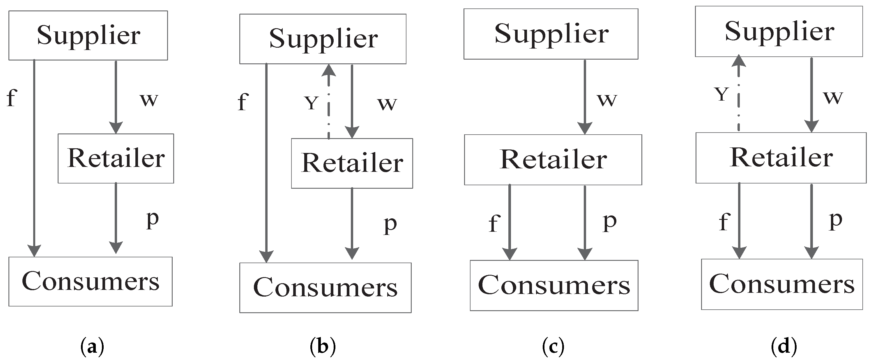
We start with the centralized mode as a benchmark in which the two parties (the supplier and retailer) are governed by a central planner. Based on who imposes the freshness-keeping effort and whether the retailer shares their private forecasting information, we divide the decentralized mode into four possible cases (see Figure 1). In brief, we use “S” or “R” to represent whether the supplier or retailer takes on the freshness-keeping effort, respectively, and “N” or “S” to indicates whether information sharing has been agreed upon or not, respectively. That is, the supplier provides the freshness-keeping effort without the retailer’s information being shared (SN), the supplier provides the freshness-keeping effort with the retailer’s information (SS), the retailer provides the freshness-keeping effort without sharing any information to the supplier (RN), and the retailer provides the freshness-keeping effort and shares their information to the supplier (RS). The optimal decisions and expected equilibrium profits under these corresponding cases are illustrated in Section 4.

3.1. Problem Description

Fresh agri-products have the characteristics of being perishable and vulnerable, which leads to high losses in the supply chain during storage, transportation and sales. In order to reduce the loss rate, the supplier or retailer must make freshness-keeping efforts, such as technological investments into storage systems, cold chain logistics and special packaging. We use f to represent the freshness-keeping effort for each product unit. The freshness-keeping effort therefore incurs an immediate freshness investment cost of $k_i{f}^2/2$, $i\in \{s,r\}$, with $k_i(>0)$ denoting the technological investment cost factor of the supply chain member i. The quadratic form of the cost reflects the general notion that it becomes increasingly more difficult and expensive to improve the freshness-keeping effort (see, e.g., [12,20]).

The market demand for fresh agri-products is affected by the degree of freshness as well as the retail price. As stated in the introduction, a higher freshness-keeping effort makes the product available to the market at a higher degree of freshness, stimulating a greater consumer willingness to buy fresh agri-products. We therefore model the consumer demand of fresh agri-products as an increasing function of the freshness-keeping effort and a decreasing function of the retail price, denoted by $q(f,p)$. For ease, we assume that the demand function takes a linear form $q(f,p)=a-p+rf$. The intercept a represents the market potential, p denotes the retail price and the parameter r$(0<r<1)$ indicates the consumer’s sensitivity to freshness. Similar demand setups are widely used in the literature (e.g., [6,26]). Fresh agricultural products are seasonal, leading to an unstable consumer demand. The unstable demand of fresh agri-products further causes volatility in the market potential. This volatility manifests as the market potential fluctuating up and down around the mean value. To model this uncertain market potential while maintaining tractability, we assume the market potential a consists of two parts, denoted by $a=a_0+\epsilon$, where $a_0$ is the deterministic part and $\epsilon$ is the random part subject to $N(0,{\sigma }_{\epsilon }^2)$. We assume that the prior distribution of a is common knowledge for both the supplier and retailer.

Regarding the uncertain market potential, as stated in the introduction, the retailer, being closer to the consumer, has access to large amounts of demand information concerning the fresh agri-products. Therefore, the retailer can further forecast the uncertain market potential based on their acquired demand information, hence obtaining a private forecast value Y concerning the market potential. The retailer’s forecast is subject to a degree of error due to biases in the availability and quality of the customer databases and market research tools. To capture this forecast error, we assume the retailer’s private forecast value $Y=a+\xi$, with $\xi$ being the random forecast error with zero mean and variance ${\sigma }_{\xi }^2$. Note that the random variables $\epsilon$ and $\xi$ are independent, thus $E\left({(Y-a_0)}^2\right|Y)={\sigma }_{\epsilon }^2+{\sigma }_{\xi }^2$. The retailer’s forecast is unbiased and hence satisfies $E\left(Y\right|a)=a_0$. Given the private forecast value Y, the expected value of the market potential can be written as $E\left(a\right|Y)=\frac{{\sigma }_{\xi }^2}{{\sigma }_{\epsilon }^2+{\sigma }_{\xi }^2}{a}_0+\frac{{\sigma }_{\epsilon }^2}{{\sigma }_{\epsilon }^2+{\sigma }_{\xi }^2}Y=T$. Let $m=\frac{{\sigma }_{\epsilon }^2}{{\sigma }_{\epsilon }^2+{\sigma }_{\xi }^2}$ ($0\le m\le 1$) be the accuracy of the retailer’s private forecast. Similar characteristics of the demand forecast have been described in previous studies [21].

Table 2. Notations and descriptions.

Notations	Descriptions
c	unit production cost
w	unit wholesale price
p	unit retail price
f	unit freshness-keeping effort
r	consumer’s sensitivity to freshness
$k_i$	technological investment cost factor of the supply chain members, $i\in \{sc,s,r\}$
${\rho }_i$	freshness-keeping effort efficiency of the supply chain members, $i\in \{sc,s,r\}$
a	uncertain market potential
$a_0$	the deterministic part of the market potential
$\epsilon$	the random part of the market potential
${\sigma }_{\epsilon }^2$	variance of the random part of the market potential
Y	forecast value of the market potential
$\xi$	the random forecast error
${\sigma }_{\xi }^2$	variance of the random forecast error
m	forecast accuracy
${\pi }_s^{(.)}$	the supplier’s profit
${\pi }_r^{(.)}$	the retailer’s profit
${\pi }_{sc}^{(.)}$	the supply chain’s profit

summarizes the notations used throughout this paper.

3.2. The Benchmark

Before analysing the decentralized mode, we start by exploring the optimal decisions and expected equilibrium profit in the centralized mode where the supplier and retailer are regarded as a whole. As such, the retailer’s demand forecasting information for the uncertain market potential can therefore be seen as common knowledge of the whole supply chain. Given the forecasting information, the expected profit function of the whole supply chain can be expressed as the following:

$$\begin{array}{c}\hfill E\left[{\pi }_{sc}^C\right|Y]=(p-c)(E\left(a\right|Y)-p+rf)-k_{sc}{f}^2/2,\end{array}$$

(1)

where the superscript “C” represents the centralized mode. In this mode, both the retail price and freshness-keeping effort are determined by a central planner to maximize the whole supply chain’s expected profits. The following theorem characterizes the optimal decisions of the central planner and the whole supply chain’s expected profits in equilibrium given the retailer’s forecasting information. For ease, we use the shorthand notation ${\rho }_i=r^2/k_i$, $i\in \{sc,s,r\}$, to represent the supply chain member’s efficiency to exert the freshness-keeping effort, and hence used throughout the paper. The proofs of the main results in this paper are shown in the Appendixes Appendix A and Appendix B.

Theorem 1.

In the centralized mode, given ${\rho }_{sc}<2$, the optimal freshness-keeping effort and optimal retail price for maximizing the supply chain’s profits are $f^C=\frac{(T-c)r}{2k_{sc}-r^2}$ and $p^C=\frac{T+c(1-{\rho }_{sc})}{2-{\rho }_{sc}}$, respectively; such that the expected profits in equilibrium are achieved by the supply chain with $E\left[{\pi }_{sc}^C\right]=\frac{m{\sigma }_{\epsilon }^2+{(a_0-c)}^2}{2(2-{\rho }_{sc})}$.

Theorem 1 suggests that the freshness-keeping effort level can be higher in equilibrium as the retailer’s private forecasting accuracy m increases (also viewed as an increase in the expected market potential T). The whole supply chain in the centralized mode is better off having a higher forecasting accuracy (m) or a larger freshness-keeping efficiency (${\rho }_{sc}<2$). The key driver of these results is that having more accurate market demand information for fresh agri-products gives the supply chain the incentive to invest more in the freshness-keeping effort, thus capturing a greater consumer demand; conversely, having a higher freshness-keeping efficiency gives the supply chain more autonomy to charge a higher retail price. The combination of the above two aspects increases the whole supply chain’s expected profit in equilibrium, while an increase in ${\rho }_{sc}$(<2) always improves operational efficiency, but can lead to a pricing disadvantage because of the higher retail price in equilibrium. Hence, the benefit of having high freshness-keeping efficiency in the centralized mode may be dominated by the loss derived from the large-scale demand decline as the retail price increases too much (i.e., ${\rho }_{sc}\ge 2$).

4. The Decentralized Mode

Having analysed the central planner’s optimal decisions in the centralized mode, we proceed to study the decentralized mode where the freshness-keeping effort taken on by either the supplier or retailer while the retailer chooses whether to share their forecasting information. We first study the optimal freshness-keeping effort level and pricing decisions under the four cases in Section 4.1. Then Section 4.2 shows a set of comparative static results on the optimal decisions and supply chain members’ equilibrium profits based on the equilibrium results under different cases.

4.1. Equilibrium Results

We start in this section by considering the situation where the supplier exerts the freshness-keeping effort given the retailer’s information sharing strategy (i.e., Case SN and Case SS, respectively). We then study the situation where the retailer exerts the freshness-keeping effort and chooses to share or not share their private forecasting information about the market potential with the supplier (i.e., Case RN and Case RS, respectively). The supply chain members’ optimal decisions and expected equilibrium profits in each case are obtained in the following.

4.1.1. Case SN

In this SN case, the supplier exerts the freshness-keeping effort and the retailer does not share their forecasting information with the supplier. Here, the supplier can only make the optimal fresh-keeping effort and wholesale price decisions based on its prior knowledge on the uncertain market potential. In other words, only the retailer has the private forecasting information about the market potential in this case. Thus, we can obtain the expected profit functions for the retailer and supplier, expressed as follows

$$E\left[{\pi }_r^{SN}\right|Y]=(p-w)(E\left(a\right|Y)-p+rf),$$

(2)

$$E\left[{\pi }_s^{SN}\right]=E[(w-c)(a_0+\epsilon -p+rf)-k_s{f}^2/2],$$

(3)

where the superscript “$SN$” denotes that the supplier takes on the freshness-keeping effort while the retailer declines to share their private forecasting information. In the SN case, the supplier according to its prior knowledge on the uncertain market potential first decides on its fresh-keeping effort level f and the wholesale price $\omega$ to offer the retailer; secondly, the retailer, after knowing the wholesale price charged by the supplier and the fresh-keeping effort level, decides on the retail price p of the fresh agri-products based on its private demand forecast information.

In this SN case, the Stackelberg game can be given as

$$\left\{\begin{array}{c}\underset{(\omega ,f)}{max}E\left[{\pi }_s^{SN}\right]\hfill \\ s.t.\underset{p}{max}E\left[{\pi }_r^{SN}\right|Y].\hfill \end{array}\right.$$

(4)

By using backward induction, we first solve the retailer’s optimization problem and obtain the optimal retail price $p^{SN}$ in terms of $\omega$ and f; then we substitute $p^{SN}(\omega ,f)$ into the supplier’s profit to solve the optimization problem, thus obtaining the optimal fresh-keeping effort level $f^{SN}$ and wholesale price ${\omega }^{SN}$. The optimal decisions and expected profits of the supply chain members in equilibrium under the SN case are presented in the first column of

Table 3. The equilibrium results of four cases in the decentralized mode.

	Case SN	Case SS	Case RN	Case RS
$f^{(.)}$	$\frac{(a_0-c)r}{4k_s-r^2}$	$\frac{(T-c)r}{4k_s-r^2}$	$\frac{(2T-a_0-c)r}{8k_r-r^2}$	$\frac{(T-c)r}{8k_r-r^2}$
$w^{(.)}$	$\frac{2a_0+c(2-{\rho }_s)}{4-{\rho }_s}$	$\frac{2T+c(2-{\rho }_s)}{4-{\rho }_s}$	$\frac{a_0+c}{2}+\frac{(2T-a_0-c){\rho }_r}{2(8-{\rho }_r)}$	$\frac{T+c}{2}+\frac{(T-c){\rho }_r}{2(8-{\rho }_r)}$
$p^{(.)}$	$\frac{2(2T+a_0+c)-(T-a_0+2c){\rho }_s}{2(4-{\rho }_s)}$	$\frac{3T+c(1-{\rho }_s)}{4-{\rho }_s}$	$\frac{2T+a_0+c}{4}+\frac{3(2T-a_0-c){\rho }_r}{4(8-{\rho }_r)}$	$\frac{6T+c(2-{\rho }_r)}{8-{\rho }_r}$
$E\left[{\pi }_s^{(.)}\right]$	$\frac{{(a_0-c)}^2}{2(4-{\rho }_s)}$	$\frac{m{\sigma }_{\epsilon }^2+{(a_0-c)}^2}{2(4-{\rho }_s)}$	$\frac{m{\sigma }_{\epsilon }^2{\rho }_r^2+16{(a_0-c)}^2}{2{(8-{\rho }_r)}^2}$	$\frac{8(m{\sigma }_{\epsilon }^2+{(a_0-c)}^2)}{{(8-{\rho }_r)}^2}$
$E\left[{\pi }_r^{(.)}\right]$	$\frac{m{\sigma }_{\epsilon }^2}{4}+\frac{{(a_0-c)}^2}{{(4-{\rho }_s)}^2}$	$\frac{m{\sigma }_{\epsilon }^2+{(a_0-c)}^2}{{(4-{\rho }_s)}^2}$	$\frac{4m{\sigma }_{\epsilon }^2+{(a_0-c)}^2}{2(8-{\rho }_r)}$	$\frac{m{\sigma }_{\epsilon }^2+{(a_0-c)}^2}{2(8-{\rho }_r)}$

${\rho }_s<4$ and ${\rho }_r<8$.

.

4.1.2. Case SS

In the SS case, the supplier takes on the freshness-keeping effort and the retailer shares its private forecasting information with the supplier. As such, the supplier in this case can determine the freshness-keeping effort and the wholesale price on the basis of the retailer’s forecast value about market potential. That is, in this case both the supplier and retailer have the forecasting information on the uncertain market potential. Hence, the two parties’ expected profit functions can be shown as

$$E\left[{\pi }_r^{SS}\right|Y]=(p-w)(E\left(a\right|Y)-p+rf),$$

(5)

$$E\left[{\pi }_s^{SS}\right|Y]=(w-c)(E\left(a\right|Y)-p+rf)-k_s{f}^2/2,$$

(6)

where the superscript “$SS$” denotes that the supplier takes on the freshness-keeping effort and the retailer shares their private forecasting information. In this case, the supplier, after knowing the shared forecasting information, determines the fresh-keeping effort level f and the wholesale price $\omega$; then the retailer decides on the optimal retail price p of the fresh agri-products given the wholesale price quoted by the supplier and the fresh-keeping effort level.

In this SS case, the Stackelberg game can be written as

$$\left\{\begin{array}{c}\underset{(\omega ,f)}{max}E\left[{\pi }_s^{SS}\right|Y]\hfill \\ s.t.\underset{p}{max}E\left[{\pi }_r^{SS}\right|Y].\hfill \end{array}\right.$$

(7)

We analyse this game model backward. We first solve the retailer’s optimization problem and obtain the optimal retail price $p^{SS}$ in terms of $\omega$ and f; then by substituting $p^{SS}(\omega ,f)$ into the supplier’s profit to solve the optimization problem, we can derive the optimal fresh-keeping effort level $f^{SS}$ and wholesale price ${\omega }^{SS}$. The optimal decisions and expected profits of the two parties in equilibrium under the SS case are shown in the second column of Table 3.

4.1.3. Case RN

In case RN, the retailer takes on the freshness-keeping effort and declines to share their forecasting information with the supplier, who then can only determine the optimal wholesale price based on their prior knowledge on the uncertain market potential. In other words, in this case, only the retailer has the private forecasting information about the market potential. Thus, we can derive the expected profit functions for the retailer and supplier as follows

$$E\left[{\pi }_r^{RN}\right|Y]=(p-w)(E\left(a\right|Y)-p+rf)-k_r{f}^2/2,$$

(8)

$$E\left[{\pi }_s^{RN}\right]=E\left[(w-c)(a_0+\epsilon -p+rf)\right],$$

(9)

where the superscript “$RN$” denotes that the retailer takes on the freshness-keeping effort while declines to share their private forecasting information. In this RN case, the supplier, using its prior knowledge on the uncertain market potential, first decides on the wholesale price $\omega$ charged by the retailer; secondly, the retailer, after observing the wholesale price offered by the supplier, decides on the fresh-keeping effort level f and retail price p of fresh agri-products based on their private demand forecasting information and the wholesale price offered by the supplier.

In this RN case, the Stackelberg game is given as

$$\left\{\begin{array}{c}\underset{\omega }{max}E\left[{\pi }_s^{RN}\right]\hfill \\ s.t.\underset{(p,f)}{max}E\left[{\pi }_r^{RN}\right|Y].\hfill \end{array}\right.$$

(10)

Using backward induction, we first solve the retailer’s optimization problem and obtain the optimal fresh-keeping effort level $f^{RN}$ and retail price $p^{RN}$; then we substitute $f^{RN}$ and $p^{RN}$ into the supplier’s profit to solve the optimization problem, thus obtaining the optimal wholesale price ${\omega }^{RN}$. The optimal decisions and expected profits of the supply chain members in equilibrium under the RN case are shown in the third column of Table 3.

4.1.4. Case RS

In the RS case, the retailer takes on the freshness-keeping effort and shares their private forecasting information with the supplier, who can then determine the wholesale price on the basis of the retailer’s forecasting information about the market potential. That is, in this case, both the supplier and retailer have the forecasting information on the uncertain market potential. Hence, the two parties’ expected profit functions can be illustrated as

$$E\left[{\pi }_r^{RS}\right|Y]=(p-w)(E\left(a\right|Y)-p+rf)-k_r{f}^2/2,$$

(11)

$$E\left[{\pi }_s^{RS}\right|Y]=E\left[(w-c)(E\left(a\right|Y)-p+rf)\right],$$

(12)

where the superscript “$RS$” denotes that the retailer takes on the freshness-keeping effort and also shares their private forecasting information. In the RS case, the supplier, after knowing the shared forecasting information, determines on the wholesale price $\omega$; then the retailer decides on the fresh-keeping effort level f and retail price p of the fresh agri-products given the wholesale price quoted by the supplier.

In this RS case, the Stackelberg game can be written as

$$\left\{\begin{array}{c}\underset{\omega }{max}E\left[{\pi }_s^{RS}\right|Y]\hfill \\ s.t.\underset{(p,f)}{max}E\left[{\pi }_r^{RS}\right|Y].\hfill \end{array}\right.$$

(13)

We analyse this game model backward. We first solve the retailer’s optimization problem and obtain the optimal fresh-keeping effort level $f^{RS}$ and retail price $p^{RS}$; then by substituting $f^{RS}$ and $p^{RS}$ into the supplier’s profit to solve the optimization problem, we derive the optimal wholesale price ${\omega }^{RS}$. The optimal decisions and expected profits of the two parties in equilibrium under the RS case are shown in the fourth column of Table 3.

4.2. Comparison and Analysis

Based on these above optimal decisions and expected equilibrium profits obtained under the four cases in the decentralized mode stated in Section 4.1, we derive several structural results on the optimal freshness-keeping effort level $f^{(.)}$, optimal price decisions $w^{(.)}$ and $p^{(.)}$, as well as the expected profits $E\left[{\pi }_s^{(.)}\right]$ and $E\left[{\pi }_r^{(.)}\right]$ in equilibrium. These results are detailed in Propositions 1–4.

Proposition 1.

Given ${\rho }_s<4$ and ${\rho }_r<8$, the optimal freshness-keeping effort level satisfies: If $T>a_0$, then $f^{SN}<f^{SS}$ and $f^{RN}>f^{RS}$; if $T<a_0$, then $f^{SN}>f^{SS}$ and $f^{RN}<f^{RS}$.

The results in Proposition 1 illustrate the effects of the retailer’s information sharing strategy on the optimal freshness effort level of the freshness-keeping effort party (the supplier or retailer) under certain conditions related to the expected market potential (captured by T). An overestimated market potential ($T>a_0$) encourages the supplier taking on the freshness-keeping effort to increase investment into freshness-keeping technologies, hence maintaining a higher freshness-keeping level if they have access to the retailer’s forecasting information. However, only an underestimated market potential ($T<a_0$) can induce the retailer taking on the freshness-keeping effort to share their private forecasting information while paying more to maintain the freshness of the agri-products. This suggests that a lower forecast in the market potential weakens the retailer’s private information advantage, such that the retailer is willing to share their information with the supplier in order to obtain a lower wholesale price, even if a higher freshness-keeping level needs to be maintained.

Proposition 2.

Given ${\rho }_s<4$ and ${\rho }_r<8$, the optimal price decisions satisfy:

(i) 

If $T>a_0$, then $w^{SN}<w^{SS}$; if $T<a_0$, then $w^{SN}>w^{SS}$;

(ii) 

If $T>a_0$, then $p^{SN}<p^{SS}$; if $T<a_0$, then $p^{SN}>p^{SS}$.

(iii) 

If $T>a_0$, then $w^{RN}<w^{RS}$ given ${\rho }_r\in (0,4)$ and $w^{RN}>w^{RS}$ given ${\rho }_r\in (4,8)$; If $T<a_0$, then $w^{RN}>w^{RS}$ given ${\rho }_r\in (0,4)$ and $w^{RN}<w^{RS}$ given ${\rho }_r\in (4,8)$.

(iv) 

If $T>a_0$, then $p^{RN}<p^{RS}$ given ${\rho }_r\in (0,2)$ and $p^{RN}>p^{RS}$ given ${\rho }_r\in (2,8)$; If $T<a_0$, then $p^{RN}>p^{RS}$ given ${\rho }_r\in (0,2)$ and $p^{RN}<p^{RS}$ given ${\rho }_r\in (2,8)$.

Proposition 2 indicates that as the supplier takes on the freshness-keeping effort, the optimal decisions of the wholesale and retailer prices are only influenced by the retailer’s information sharing strategy under certain conditions relating to the expected market potential (T). As indicated by parts (i) and (ii) of Proposition 2, an overestimated (underestimated) market potential makes the wholesale and retail prices in equilibrium to increase (decrease) if the retailer shares their private forecasting information, while parts (iii) and (iv) of Proposition 2 establish that the impact of the retailer’s information sharing strategy on the optimal wholesale and retail price decisions depends not on the expected market potential and the freshness-keeping efficiency (${\rho }_r$). Specifically, given an overestimated market potential, a lower (higher) freshness-keeping efficiency results in higher (lower) wholesale and retail prices in equilibrium when the retailer chooses to share their private forecasting information; on the other hand, given an underestimated market potential, a lower (higher) freshness-keeping efficiency results in lower (higher) wholesale and retail prices in equilibrium when the retailer shares their forecasting information. Our analysis shows that the retailer taking on the freshness-keeping effort is able to exert greater influence over the optimal wholesale and retail prices. This is reflected in the retailer’s ability to access the private forecasting information and the operational efficiency with which it exerts its preservation effort.

Proposition 3.

Given ${\rho }_s$ and ${\rho }_r$, then the following statements hold true:(i)$E\left[{\pi }_s^{SN}\right]<E\left[{\pi }_s^{SS}\right]$ for all ${\rho }_s\in (0,4)$;(ii)$E\left[{\pi }_s^{RN}\right]<E\left[{\pi }_s^{RS}\right]$ if and only if ${\rho }_r\in (0,4)$; otherwise, $E\left[{\pi }_s^{RN}\right]>E\left[{\pi }_s^{RS}\right]$ if and only if ${\rho }_r\in (4,8)$.

Part (i) of Proposition 3 indicates that as the retailer shares their private forecasting information profit improvement in equilibrium is always available to the supplier taking on the freshness-keeping effort given that their freshness-keeping efficiency (${\rho }_s$) does not exceed the threshold ${\rho }_s\in (0,4)$, as stated in Table 3. One might anticipate that as the freshness-keeping efficiency increases, a higher expected profit in equilibrium can be achieved by the supplier when it also obtains the retailer’s private forecasting information. However, even when receiving the private forecasting information the supplier is worse off as the freshness-keeping efficiency is large with ${\rho }_r\in (4,8)$, as described in part (ii) of Proposition 3. This demonstrates that the supplier may benefit more from the spillover effect resulting from the retailer’s higher operational efficiency which outweighs their information disadvantage due to asymmetric information as the retailer forecasts more demand.

Proposition 4.

Given ${\rho }_s$ and ${\rho }_r$, then the following statements hold true: (i)$E\left[{\pi }_r^{SN}\right]>E\left[{\pi }_r^{SS}\right]$ if and only if ${\rho }_s\in (0,2)$; otherwise, $E\left[{\pi }_r^{SN}\right]<E\left[{\pi }_r^{SS}\right]$ if and only if ${\rho }_s\in (2,4)$; (ii)$E\left[{\pi }_r^{RN}\right]>E\left[{\pi }_r^{RS}\right]$ for all ${\rho }_r\in (0,8)$.

Part (i) of Proposition 4 demonstrates that when the supplier takes on the freshness-keeping effort, a freshness-keeping efficiency (${\rho }_s$) within the range $(0,2)$ makes keeping the private forecasting information more likely to be favoured by the retailer. However, as ${\rho }_s$ increases within the range $(2,4)$, the freshness-keeping efficiency encourages the retailer to share its private forecasting information because of the spillover effect caused by the supplier’s higher operational efficiency—case SS indicated in part (i) of Proposition 4. Intuitively, when taking on the freshness-keeping effort, having the private forecasting information tends to be preferable for the retailer for all ${\rho }_r\in (0,8)$, who hence has more initiative and decision-making power in its operations, as shown in part (ii) of Proposition 4.

5. The Contract Coordination Mode

As established in Proposition 4 of Section 4.2, the retailer taking on the freshness-keeping effort is always reluctant to share their private information as $E\left[{\pi }_r^{RN}\right]>E\left[{\pi }_r^{RS}\right]$ for all ${\rho }_r\in (0,8)$. We can also derive ${\mathrm{\Pi }}_{sc}^{RS}<{\mathrm{\Pi }}_{sc}^{RN}$ from Table 3 where ${\mathrm{\Pi }}_{sc}^{RS}=E\left[{\pi }_s^{RS}\right]+E\left[{\pi }_r^{RS}\right]$ and ${\mathrm{\Pi }}_{sc}^{RN}=E\left[{\pi }_s^{RN}\right]+E\left[{\pi }_r^{RN}\right]$, such that information sharing is always detrimental to the revenue improvement of the whole supply chain when the freshness-keeping effort is exerted by the retailer in the decentralized mode. On the other hand, when the supplier takes on the freshness-keeping effort, while the entire supply chain may benefit from the retailer’s information sharing strategy, that is, ${\mathrm{\Pi }}_{sc}^{SN}<{\mathrm{\Pi }}_{sc}^{SS}$, it still falls far short of the supply chain’s benefit of the centralized scenario (i.e., ${\mathrm{\Pi }}_{sc}^C$). This is shown in Section 3.2, which is the most efficient mode but difficult to achieve in reality. Besides the above results, it is obvious that ${\mathrm{\Pi }}_{sc}^{RS}<{\mathrm{\Pi }}_{sc}^{SS}<{\mathrm{\Pi }}_{sc}^C$ by comparison.

Hence, the supplier is motivated to encourage the retailer to share their private information, we then design three incentive contracts to facilitate supply chain coordination and to further improve the operational efficiency of the decentralized mode based on the SS case. These three incentive contracts include (i) cost-sharing, (ii) revenue-sharing and (iii) revenue-and-cost-sharing contracts. We first study the equilibrium results of these three incentive contracts in Section 5.1. Then Section 5.2 compares the supply chain members’ profits in equilibrium between this contract coordination mode shown in Section 5.1 and the decentralized mode characterized in Section 4.1.

5.1. Equilibrium Results

In this section, we first focus on the cost-sharing contract in which the immediate freshness investment cost of $k_s{f}^2/2$, with $k_s$ (>0) denoting the technological investment cost factor of the supplier, is shared by the supplier and retailer. $\lambda \in (0,1)$ denotes the proportion of freshness investment costs covered by the retailer, and hence the supplier takes on the remaining $(1-\lambda )$ portion of freshness investment costs. Then, the supplier and retailer’s expected profit functions are shown as

$$E\left[{\pi }_s^{cs}\right|Y]=(w-c)(E\left(a\right|Y)-p+rf)-(1-\lambda )k_s{f}^2/2,$$

(14)

$$E\left[{\pi }_r^{cs}\right|Y]=(p-w)(E\left(a\right|Y)-p+rf)-\lambda k_s{f}^2/2,$$

(15)

where the superscript “cs” represents the use of a cost-sharing contract. The game order in this case is similar to that of the SS case, and thus the equilibrium results obtained by adopting backward induction are shown in the first column of

Table 4. The equilibrium outcomes of the three incentive contracts.

	Cost-Sharing	Revenue-Sharing	Revenue-and-Cost-Sharing
$f^{(.)}$	$\frac{(T-c)r}{4k_s(1-\lambda )-r^2}$	$\frac{(T-c)r}{2k_s(1+\eta )-r^2}$	$\frac{(T-c)r}{2k_s(1+\alpha )(1-\beta )-r^2}$
$w^{(.)}$	$\frac{2(1-\lambda )(T+c)-c{\rho }_s}{4(1-\lambda )-{\rho }_s}$	$\frac{\eta (2\eta T+c)-c{\rho }_s\left)\right)}{2(1+\eta )-{\rho }_s}$	$\frac{\alpha (2(1-\beta )(\alpha T+c)-c{\rho }_s)}{2(1+\alpha )(1-\beta )-{\rho }_s}$
$p^{(.)}$	$\frac{(1-\lambda )(3T+c)-c{\rho }_s}{4(1-\lambda )-{\rho }_s}$	$\frac{(1+2\eta )T+c(1-{\rho }_s)}{2(1+\eta )-{\rho }_s}$	$\frac{(1-\beta )((1+2\alpha )T+c)-c{\rho }_s}{2(1+\alpha )(1-\beta )-{\rho }_s}$
$E\left[{\pi }_s^{(.)}\right]$	$\frac{(1-\lambda )(m{\sigma }_{\epsilon }^2+{(a_0-c)}^2)}{4(1-\lambda )-{\rho }_s}$	$\frac{m{\sigma }_{\epsilon }^2+{(a_0-c)}^2}{2(2(1+\eta )-{\rho }_s)}$	$\frac{(1-\beta )(m{\sigma }_{\epsilon }^2+{(a_0-c)}^2)}{2(2(1+\alpha )(1-\beta )-{\rho }_s)}$
$E\left[{\pi }_r^{(.)}\right]$	$\frac{(\lambda {\rho }_s-2{(1-\lambda )}^2)(m{\sigma }_{\epsilon }^2+{(a_0-c)}^2)}{2{(4(1-\lambda )-{\rho }_s)}^2}$	$\frac{\eta (m{\sigma }_{\epsilon }^2+{(a_0-c)}^2)}{{(2(1+\eta )-{\rho }_s)}^2}$	$\frac{(2\alpha (1+{\beta }^2)-\beta (4\alpha +{\rho }_s))(m{\sigma }_{\epsilon }^2+{(a_0-c)}^2)}{2{(2(1+\alpha )(1-\beta )-{\rho }_s)}^2}$

.

Secondly, we consider the revenue-sharing contract in which the supplier incurs an immediate freshness investment cost of $k_s{f}^2/2$ and can also obtain a proportion $(1-\eta )$ of the partial sales revenue from the retailer, who then only holds the remaining proportion $\eta \in (0,1)$ of the sales revenue. Hence, the corresponding expected profit functions of the supplier and retailer are expressed as follows:

$$E\left[{\pi }_s^{re}\right|Y]=((1-\eta )p+w-c)(E\left(a\right|Y)-p+rf)-k_s{f}^2/2,$$

(16)

$$E\left[{\pi }_r^{re}\right|Y]=(\eta p-w)(E\left(a\right|Y)-p+rf).$$

(17)

where the superscript “re” captures the revenue-sharing contract. The game order in this revenue-sharing contract case is similar to that of the SS case, and thus the equilibrium results derived by using backward induction are shown in the second column of Table 4.

Thirdly, we study the revenue-and-cost-sharing contract in which the supplier and retailer not only share the retailer’s sales revenue but the immediate freshness investment cost of $k_s{f}^2/2$. We refer to $\alpha \in (0,1)$ as the percent sales revenue retained by the retailer, then the supplier receives the remaining $(1-\alpha )$ portion of the retailer’s sales revenue. Let $\beta \in (0,1)$ represent the percentage of the freshness investment cost taking on by the retailer, and the remaining $(1-\beta )$ portion is taking on by the supplier. Further, the supplier and retailer’s corresponding expected profit functions can be given by

$$E\left[{\pi }_s^{rc}\right|Y]=((1-\alpha )p+w-c)(E\left(a\right|Y)-p+rf)-(1-\beta )k_s{f}^2/2,$$

(18)

$$E\left[{\pi }_r^{rc}\right|Y]=(\alpha p-w)(E\left(a\right|Y)-p+rf)-\beta k_s{f}^2/2,$$

(19)

where the superscript “rc” represents the revenue-and-cost-sharing contract. The game order in this revenue-and-cost-sharing contract case is similar to that of the SS case, and the equilibrium results can be obtained by using backward induction, as shown in the third column of Table 4.

Lemma 1.

When the incentive contract is adopted in equilibrium:

(i) 

Under the cost-sharing contract, if $\frac{2{(1-\lambda )}^2}{\lambda }<{\rho }_s<4(1-\lambda )$ is satisfied, then $E\left[{\pi }_s^{cs}\right]$ and $E\left[{\pi }_r^{cs}\right]$ increases in ${\rho }_s$ and m;

(ii) 

Under the cost-sharing contract, if ${\rho }_s<2(1+\eta )$ is satisfied, then $E\left[{\pi }_s^{re}\right]$ and $E\left[{\pi }_r^{re}\right]$ increase in ${\rho }_s$ and m;

(iii) 

Under the cost-sharing contract, if ${\rho }_s<2(1+\alpha )(1-\beta )$ is satisfied, then $E\left[{\pi }_s^{rc}\right]$ and $E\left[{\pi }_r^{rc}\right]$ increases in ${\rho }_s$ and m.

Lemma 1 shows that all three types of incentive contracts can work under certain conditions based on the SS case where the supplier takes on the freshness-keeping effort and the retailer shares its private forecasting information. Specifically, more accurate forecast information (m is larger) or a greater freshness-keeping efficiency (${\rho }_s$) induces higher freshness of fresh agri-products and therefore potentially encourages more consumers to buy fresh agri-products. This consequently achieves higher returns for the supplier and retailer (as reflected by larger $E\left[{\pi }_s^{(.)}\right]$ and $E\left[{\pi }_r^{(.)}\right]$).

5.2. Comparison and Analysis

Having derived and analysed the equilibrium outcomes of the three incentive contracts, we proceed to compare these equilibrium results between contract coordination mode shown in Section 5.1 and the decentralized mode characterized in Section 4.1. The following proposition proves that the contract coordination mode outperforms the decentralized mode if the contract parameters fall within the reasonable ranges.

Proposition 5.

By comparing the contract coordination and decentralized modes, we can find that

(i)

The supplier and retailer are better off with the cs contract when $\lambda \in (0,\Phi )$ with $\Phi =\frac{4{\rho }_s\sqrt{64+{\rho }_s^2}+{\rho }_s\sqrt{{\rho }_s(64-24{\rho }_s+{\rho }_s^3)}-{\rho }_s^2(4+{\rho }_s)+32}{4({\rho }_s^2+8(1-{\rho }_s))}$;

(ii)

The supplier and retailer are better off with the re contract when $\eta \in \left(0,\frac{{(2-{\rho }_s)}^2}{4}\right)$;

(iii)

The supplier and retailer are better off with the rc contract when $\alpha \in \left(\frac{2+\beta ({\rho }_s-2)}{2(1+\beta )},1\right)$.

The above proposition states that regardless of the type of incentive contract, the supplier and retailer are likely to achieve improved profits such that supply chain coordination is realized via designing incentive contracts. Whether the supplier and retailer hold the identical preferences for incentive contracts depends on the ranges of those contract parameters. Concretely, the retailer will choose to accept the cs contract and share its private forecasting information when the proportion of freshness investment costs $\lambda$ lies within $(0,\Phi )$, as indicated in part (i) of Proposition 5. When adopting the re contract, similar findings in part (ii) of Proposition 5 can also be obtained and the range of contract parameters remain structurally the same as in the cs contract, with the difference being that the retailer’s sales revenue rather than the supplier’s freshness investment costs are shared. That is, the proportion of sales revenue needs to satisfy $\eta \in \left(0,\frac{{(2-{\rho }_s)}^2}{4}\right)$. Part (iii) of Proposition 5 shows that the rc contract can improve the two parties’ profits in the supply chain as the contract parameters, in relation to revenue and cost sharing, meet a certain condition with $\alpha \in \left(\frac{2+\beta ({\rho }_s-2)}{2(1+\beta )},1\right)$.

Notably, taking on the freshness-keeping effort enables the supplier to possess more initiative to facilitate supply chain coordination. This is because the freshness-keeping efficiency (${\rho }_s$) has an influence on the ranges of the above contract parameters. An increase in ${\rho }_s$ improves the operational efficiency in freshness-keeping and consequently enlarges (narrows) the scope of the cs contract parameter $\lambda$ (re contract parameter $\eta$). This shows that the improvement in operation efficiency makes the supplier have a greater voice in terms of bearing less of the freshness-keeping costs or holding more shared benefits from the retailer. However, under the rc contract, an increase in ${\rho }_s$ makes the supplier voluntarily transfer some advantages to the retailer, which is reflected in that the rc contract parameter $\alpha$ can achieve a larger value given the cost-sharing parameter $\beta$, such that the latter can retain a greater sales revenue.

6. Numerical Study

To demonstrate the obtained theoretical results in Section 4 and Section 5 and derive more managerial insights, numerical examples are explored in this section. The above propositions, including the freshness-keeping efficiency impact on the wholesale price, retail price, the supplier and retailer’s equilibrium profits, and the information sharing within the four decentralized mode cases, are visualized in Section 6.1. Furthermore, Section 6.2 visualizes the impacts of the three types of contract parameters on the supply chain members’ profits in equilibrium in the contract coordination mode.

In what follows, we give the basic parameter values and some figures to depict the propositions in our paper. The parameters are set as follows: $T=20,a_0=15,c=1,\rho =1,m=0.8,{\sigma }_{\epsilon }=3,\lambda =0.2,\eta =0.8,\alpha =0.8,$ and $\beta =0.1$. Note that the above parameter values meet all the aforementioned conditions stated in the corresponding situations.

6.1. The Impact of the Freshness-Keeping Efficiency in the Decentralized Mode

In this subsection, we demonstrate the impact of the freshness-keeping efficiency on the optimal price decisions and equilibrium profits in Figure 2 and Figure 3, as well as the retailer’s information sharing strategy in Figure 4 when the supplier taking in the freshness-keeping effort.

As seen in Figure 2a, whether the retailer shares their private forecasting information or not, the larger value of the supplier’s freshness-keeping efficiency ${\rho }_s$, the higher the wholesale price $w^{(.)}$ and retail price $p^{(.)}$ in the SN and SS cases, as indicated in parts (i) and (ii) of Proposition 2. Moreover, it is intuitive that the profit margins, characterized by $p^{(.)}-w^{(.)}$ in the SN and SS cases, increase in ${\rho }_s$, therefore improving the supply chain members’ profits in equilibrium as the freshness-keeping efficiency ${\rho }_s$ increases. As depicted in Figure 2b, the supplier is always better off having the retailer’s forecasting information as ${\rho }_s$ increases, while information sharing tends to only be preferable to the retailer if the freshness-keeping efficiency exceeds a certain threshold ${\rho }_s^{\prime }=2$. This echoes our analytical findings in part (i) of Propositions 3 and 4.

According to Figure 3a, as the retailer’s freshness-keeping efficiency ${\rho }_r$ increases, the wholesale price $w^{(.)}$ and retail price $p^{(.)}$ become larger in the RN and RS cases. In particular, the changes in $w^{(.)}$ and $p^{(.)}$ are also affected by the retailer’s information sharing strategy, consistent with the results in parts (iii) and (iv) of Proposition 2. We can readily conclude that there exist two thresholds, ${\rho }_r^1=2$ and ${\rho }_r^2=4$, such that the retailer could pay a lower wholesale price and reach a higher retail price if ${\rho }_r$ lies in the interval $[{\rho }_r^1,{\rho }_r^2]$ as information sharing is absent. From parts (ii) of Propositions 3 and 4, we obtain a set of results by comparing the supply chain members’ equilibrium profits in the RN and RS cases, based on which we conduct a numerical study as shown in Figure 3b. This presents that the supplier can only be better with the retailer’s private forecasting information if the freshness-keeping efficiency held by the retailer is lower (i.e., ${\rho }_r\in (0,4)$), while the retailer is more likely to decline sharing their information when taking on the freshness-keeping effort themselves.

Based on Propositions 3 and 4 stated in Section 4.2, we find that the retailer’s information sharing strategy depends on the value of the freshness-keeping efficiency. Specifically, the retailer still fails to benefit from an information sharing strategy when taking on the freshness-keeping effort. On the contrary, when the supplier takes on the freshness-keeping effort, the retailer can be better off sharing their private forecasting information, as the freshness-keeping efficiency lies within a certain range (i.e., ${\rho }_s\in (2,4)$). Hence, Figure 4 visualizes this result and the threshold ${\rho }_s^{\prime }=2$ which highlights the retailer’s choice of information sharing strategy in a more intuitive way.

6.2. The Impact of the Sharing Proportion in the Contract Coordination Mode

In this subsection, we demonstrate the influence of the three types contract parameters on the supplier and retailer’s equilibrium profits in the contract coordination mode based on the equilibrium outcomes presented in Table 4.

In Figure 5, we plot the supply chain members’ expected profits $E\left[{\pi }_s^{cs}\right]$ and $E\left[{\pi }_r^{cs}\right]$ in equilibrium as the cost-sharing contract parameter $\lambda$ varies given a certain value of freshness-keeping efficiency (${\rho }_s=0.8$ or ${\rho }_s=1$) (see, e.g., [4,6]). As shown in Figure 5a, when the freshness investment cost covered by the retailer becomes higher, that is, $\lambda$ becomes larger, the supplier’s cost pressure is reduced accordingly, improving their profits. In contrast, the retailer is worse off as the cost-sharing ratio increases. This is intuitive in the current supply chain operation management study related to the cost-sharing coordination contract. By comparing Figure 5a,b, we find the effectiveness of the freshness-keeping efficiency ${\rho }_s$ that alleviates the profit gap to some extent between the supplier and retailer caused by the cost-sharing contracts. This can be reflected by the reduction in the distance between the two equilibrium profit curves from Figure 5a,b.

As established in Figure 6, we plot the supply chain members’ expected profits (i.e., $E\left[{\pi }_s^{re}\right]$ and $E\left[{\pi }_r^{re}\right]$) in equilibrium as the revenue-sharing contract parameter $\eta$ varies given a certain value of the freshness-keeping efficiency (${\rho }_s=0.8$ or ${\rho }_s=1$). As $\eta$ increases, the supplier obtains less sales revenue from the retailer while the latter holds more of the remaining sales revenue; hence, the supplier is worse off and the retailer is better off with an increase in $\eta$. Moreover, the effect of the freshness-keeping efficiency ${\rho }_s$ can be attained by comparing Figure 6a,b, indicating that the increase in the freshness-keeping efficiency makes the change in equilibrium profits more obvious, hence narrowing the profit gap between the supplier and retailer.

Figure 7 depicts the expected profits of the supplier (i.e, $E\left[{\pi }_s^{rc}\right]$), the retailer (i.e, $E\left[{\pi }_r^{rc}\right]$) and the whole supply chain in equilibrium as the revenue-and-cost-sharing contract parameters $\alpha$ and $\beta$ vary. As shown in Figure 7a, the supplier and retailer’s expected equilibrium profits are represented by the white and blue surfaces, respectively. Given the cost-sharing parameter $\beta$, the supplier’s equilibrium profits increase as $\alpha$ increases, while the retailer’s profits in equilibrium first increase until they reach a maximum and then decrease. Given the revenue-sharing value $\alpha$, the supplier’s equilibrium profits gradually decrease as $\beta$ increases; this is accompanied by an increase in the retailer’s equilibrium profits. Hence, the changes in the contract parameters $\alpha$ and $\beta$ lead to opposite effects on the supplier and retailer’s profits in equilibrium. In particular, we also find that the revenue-and-cost-sharing contract may work if the contract parameters $\alpha$ and $\beta$ are within a moderate range, as established in Figure 7b.

7. Conclusions and Future Research

To investigate the supply chain members’ optimal freshness-keeping effort decisions and the retailer’s private forecasting information sharing strategies, we considered and compared four cases to investigate the supply chain members’ strategies based on who exerts the freshness-keeping effort and whether the retailer shares its private forecasting information. Furthermore, the contract coordination mode including three incentive contracts were designed to facilitate supply chain coordination. We studied how different cases and contracts affect supply chain members’ decisions regarding the freshness-keeping effort level, wholesale price, retail price, as well as the respective expected profits in equilibrium. In addition to an analytical investigation, we also conducted a numerical study to enrich our analysis.

The model solutions within the four cases in the decentralized mode demonstrate that, when the supplier takes on the freshness-keeping effort, the optimal freshness-keeping effort level, wholesale price and retail price are only influenced by the retailer’s information sharing strategy, reflected in the value of the expected market potential; however, when the retailer takes on the freshness-keeping effort, the impact of the retailer’s information sharing strategy on the optimal wholesale and retail price decisions depends on the expected market potential and the retailer’s freshness-keeping efficiency. By examining the impact of the retailer’s information sharing strategy on both supply chain members’ expected profits in equilibrium, we find that sharing information does not always benefit the supplier given a larger freshness-keeping efficiency when the retailer exerts the freshness-keeping effort. Moreover, declining to share the forecasting information tends to always be preferable for the retailer taking on the freshness-keeping effort. After deriving the equilibrium results of the three incentive contracts in the coordination mode, we compared the supplier and retailer’s expected profits in equilibrium between the decentralized and coordination modes. We show that, based on Case SS, the effective incentive contracts may work in facilitating supply chain coordination, consequently improving profits for the supplier and retailer. By conducting a numerical study, the above results were established in a more intuitive way. We found that the three types of contract parameters in the coordination mode all resulted in opposite effects for both parties’ expected profits in equilibrium. In particular, the freshness-keeping efficiency exerted by the supplier reduced the profit gap between the supplier and retailer in the cs and re contracts.

This paper provides a more comprehensive perspective of the industry’s practical behaviour in an FAPSC consistent with the objective perceptions. According to the above analysis and conclusions, we provide several applications of this research related to the theoretical and practical aspects. First, the construction of a Stackelberg game model can effectively capture the characteristics of the fresh agri-products trade and the decision-making behaviour of the members in an FAPSC. Further, the model can objectively describe and reflect the industry’s practices. Second, the design of the contract mechanism including three incentive contracts is regarded as an effective method for supply chain members to achieve great profit improvements, providing managerial implications and a realization path for their long-term cooperation in a win–win situation. Third, the adoption of the numerical simulation method via Matlab can clearly and intuitively express the research results.

We note a few limitations of our paper and provide several extended directions for future research. First, we investigated two freshness-keeping effort methods exerted by the supplier or retailer; moreover, our model can be extended to consider a third party who takes on the freshness-keeping effort and analyse the three parties’ decisions accordingly. Second, we analysed the optimization and coordination of a two-echelon supply chain comprising one supplier and one retailer, while the consumer’s utility was not involved. Future studies should examine an FAPSC by taking the consumer’s utility and surplus into consideration. Finally, we assume the supplier and retailer are both risk-neutral and additional risk types are not analysed which could be explored in future research.