Multi-Objective LQG Design with Primal-Dual Method

Abstract

The objective of this paper is to investigate a multi-objective linear quadratic Gaussian (LQG) control problem. Specifically, we examine an optimal control problem that minimizes a quadratic cost over a finite time horizon for linear stochastic systems subject to control energy constraints. To tackle this problem, we propose an efficient bisection line search algorithm that outperforms other approaches such as semidefinite programming in terms of computational efficiency. The primary idea behind our algorithm is to use the Lagrangian function and Karush–Kuhn–Tucker (KKT) optimality conditions to address the constrained optimization problem. The bisection line search is employed to search for the Lagrange multiplier. Furthermore, we provide numerical examples to illustrate the efficacy of our proposed methods.

1. Introduction

Optimal control of dynamical systems has long been one of the fundamental problems in the control community [1,2,3,4]. Among various optimal control scenarios, the linear quadratic Gaussian (LQG) control problem is our main concern. It covers various applications such as mobile robots, an industrial quality control system, and flight control to name just a few. The LQG problem can be efficiently solved using the classical dynamic programming and Riccati equation [1,2]. In many applications, however, there exist several possibly competing objectives that require behaviors that mediate among them. Sometimes, those multiple objectives can be formulated as constraints; for instance, bounds on different objectives, risk measures or costs. In the classical dynamic programming, multiple objectives can be encoded into the cost to be minimized. However, since they are blended into a single cost, designing a policy that satisfies constraints or minimizes multiple objectives is challenging. In this respect, an optimization-based multi-objective LQG design provides more potentials than the traditional dynamic-programming-based approaches by leveraging the existing constrained optimization algorithms and theories [5].

The emergence of convex optimization [5] and semidefinite programming (SDP) [6] techniques in control analysis and design promoted new optimization formulations of control problems [7,8,9,10,11,12,13,14,15,16,17,18,19]. They have also provided greater convenience and flexibility in control design with various objectives and constraints. However, when the size of the problem is large, the computational complexity of such SDP-based algorithms is known to explode quickly, and it makes the problem numerically inefficient.

Motivated by the discussions above, this paper’s primary objective is to investigate a numerically efficient algorithm for linear quadratic Gaussian (LQG) problems that have an energy constraint, utilizing optimization theory and Lagrangian duality. The problem has many applications such as the building control problems [20,21,22], where limited resources are allowed for the control task. To find an optimal solution to the problem, we suggest a simple and efficient bisection line search algorithm whose computational complexity is in general lower than SDP-based methods. The main idea is to formulate a constrained optimization problem, and then use the Lagrangian function and Karush–Kuhn–Tucker (KKT) optimality conditions [23] to solve the constrained optimization problem. The Lagrange multiplier is searched using the bisection line search. A numerical example of a building control problem is given to demonstrate the effectiveness of the proposed methods.

Some lists of related works are summarized as follows. Ref.  [24] presented a technique to compute the explicit state-feedback solution to both the finite and infinite horizon optimal linear quadratic regulator (LQR) problem subject to state and input constraints. They showed that this closed form solution is piecewise linear and continuous. Ref. [25] developed efficient algorithms to compute such piecewise linear solutions of the constrained LQR problems. The constrained LQR problem was also considered for hybrid systems in [26]. Ref. [27] presented an efficient algorithmic solution to the infinite horizon LQR problem for a discrete-time SISO plant subject to constraints on a scalar variable. The solution to the corresponding quadratic programming problem is based on the active set method and on dynamic programming. Ref. [28] considered a feedback control problem such that the controlled signals have a guaranteed maximum peak value in response to arbitrary but bounded energy exogenous inputs. Ref. [29] proposed a new SDP formulation, where the finite-horizon LQG problem was converted into the optimal covariance matrix selection problem, and addressed energy constrained LQG. Other SDP formulations of control problems with various constraints have been developed in several papers [7,29,30,31,32] to name just a few.

Considering types of constraints, systems, and problems, the most related previous work is [29], which considers energy bounds on the weighted state and control input, and uses SDP solutions. Our main contribution is the development of a simple and numerically efficient algorithm for the energy bounded LQG problem, which does not rely on SDPs. The new method uses a simple and efficient bisection line search algorithm whose computational complexity is in general lower than SDP-based methods. We demonstrate the efficiency of the algorithm through a numerical example.

Notation 1. 

The adopted notation is as follows: $\mathbb{N}$ and ${\mathbb{N}}_{+}$: sets of non-negative and positive integers, respectively; $\mathbb{R}$: set of real numbers; ${\mathbb{R}}_{+}$: set of non-negative real numbers; ${\mathbb{R}}_{++}$: set of positive real numbers; ${\mathbb{R}}^n$: n-dimensional Euclidean space; ${\mathbb{R}}^{n\times m}$: set of all $n\times m$ real matrices; $A^T$: transpose of matrix A; $A^{-T}$: transpose of matrix $A^{-1}$; $A\succ 0$ ($A\prec 0$, $A⪰0$, and $A⪯0$, respectively): symmetric positive definite (negative definite, positive semi-definite, and negative semi-definite, respectively) matrix A; $I_n$: $n\times n$ identity matrix; ${\mathbb{S}}^n$: symmetric $n\times n$ matrices; ${\mathbb{S}}_{+}^n$: cone of symmetric $n\times n$ positive semi-definite matrices; ${\mathbb{S}}_{++}^n$: symmetric $n\times n$ positive definite matrices; and $Tr\left(A\right)$: trace of matrix A.

2. Finite-Horizon LQG Problem

Consider the stochastic linear time-invariant (LTI) system

$$\begin{array}{cc}\hfill & x(k+1)=Ax\left(k\right)+Bu\left(k\right)+w\left(k\right),\hfill \end{array}$$

(1)

where $k\in \mathbb{N}$, $A\in {\mathbb{R}}^{n\times n}$, $B\in {\mathbb{R}}^{n\times m}$ are system matrices, $x\left(k\right)\in {\mathbb{R}}^n$ is the state vector, $u\left(k\right)\in {\mathbb{R}}^m$ is the input vector, $x\left(0\right)\sim \mathcal{N}(z,V)$ and $w\left(k\right)\sim \mathcal{N}(0,W)$ are mutually independent Gaussian random vectors so that $\mathbb{E}\left[x\right(0\left)\right]=z$, $\mathbb{E}\left[w\right(k\left)\right]=0$, $\mathbb{E}[(x\left(0\right)-z){(x\left(0\right)-z)}^T]=V$, and $\mathbb{E}[w\left(k\right)w{\left(k\right)}^T]=W$. In this paper, we consider the following multi-objective finite-horizon LQG problem:

Problem 1 

(Multi-objective LQG problem). Solve

$$\begin{array}{cc}\hfill & \underset{F_0,\dots ,F_{N-1}\in {\mathbb{R}}^{m\times n}}{min}\mathbb{E}[x{\left(k\right)}^T{Q}_{f}x\left(k\right)]+\sum _{k=0}^{N-1}\mathbb{E}\left[{\left[\begin{array}{c}x\left(k\right)\\ u\left(k\right)\end{array}\right]}^T\left[\begin{array}{cc}{Q}_k& 0\\ 0& R_k\end{array}\right]\left[\begin{array}{c}x\left(k\right)\\ u\left(k\right)\end{array}\right]\right]\hfill \\ \hfill & \mathrm{subject}\mathrm{to}\hfill \\ \hfill & x(k+1)=Ax\left(k\right)+Bu\left(k\right)+w\left(k\right),\hfill \\ \hfill & u\left(k\right)=F_{k}x\left(k\right),\hfill \\ \hfill & \mathbb{E}[x{\left(k\right)}^T{\tilde{Q}}_{f}x\left(k\right)]+\sum _{k=0}^{N-1}\mathbb{E}\left[{\left[\begin{array}{c}x\left(k\right)\\ u\left(k\right)\end{array}\right]}^T\left[\begin{array}{cc}{\tilde{Q}}_k& 0\\ 0& {\tilde{R}}_k\end{array}\right]\left[\begin{array}{c}x\left(k\right)\\ u\left(k\right)\end{array}\right]\right]\le \gamma .\hfill \end{array}$$

Note that the second objective is encoded into the inequality instead of the objective function. The problem may be useful in many optimal control applications, for example, the building control problem [20,21,22], where the goal is to reduce the indoor temperature tracking error as much as possible while using limited energy for the control input within a certain time horizon.

Example 1. 

Consider a room’s thermal dynamic model expressed as (1) with

$$\begin{array}{cc}\hfill & A=\left[\begin{array}{cccc}0.9500& 0.0250& 0.0250& 0\\ 0.0250& 0.9750& 0& 0\\ 0& 0& 1& 0\\ 0& 0& 0& 1\end{array}\right],B=\left[\begin{array}{c}0.0250\\ 0\\ 0\\ 0\end{array}\right],\hfill \end{array}$$

where $x_1\left(k\right)$ is the indoor air temperature (${}^{\circ }\mathrm{C}$), $x_2\left(k\right)$ is the wall temperature (${}^{\circ }\mathrm{C}$), $x_3\left(k\right)$ is the outdoor air temperature (${}^{\circ }\mathrm{C}$), $x_4\left(k\right)$ is the reference temperature (${}^{\circ }\mathrm{C}$), $u\left(k\right)$ (W) is the control input, which represents the amount of energy injected into the room. For instance, when the goal is to heat the room, $u\left(k\right)>0$, while $u\left(k\right)<0$ when the objective is to cool the room. The outdoor air temperature and reference temperature are kept constant ($30{}^{\circ }\mathrm{C}$ and $24{}^{\circ }\mathrm{C}$, respectively) over time. To this end, the initial state should be deterministic and fixed, and the last element of the noise $w\left(k\right)$ should be zero over time. In this case, the initial state should be set to be

$$x\left(0\right)={\left[\begin{array}{cccc}{x}_1\left(0\right)& x_2\left(0\right)& 30& 24\end{array}\right]}^T$$

where $x_1\left(0\right)$ is the initial indoor air temperature, and $x_2\left(0\right)$ is the initial wall temperature. We want to enforce the indoor temperature to track the reference temperature $24{}^{\circ }\mathrm{C}$ as close as possible while satisfying the total input energy constraint

$$\mathbb{E}\left[\sum _{k=0}^{N-1}u{\left(k\right)}^2\right]\le \gamma ,$$

The problem can be formulated as Problem 1 with

$$\begin{array}{cc}\hfill Q_f=& Q_k={\left[\begin{array}{cccc}1& 0& 0& -1\end{array}\right]}^T\left[\begin{array}{cccc}1& 0& 0& -1\end{array}\right],\hfill \\ \hfill R_k=& 0,k\in \{0,1,\dots ,N-1\}\hfill \end{array}$$

and

$${\tilde{Q}}_f={\tilde{Q}}_k=0,{\tilde{R}}_k=1,k\in \{0,1,\dots ,N-1\}$$

The cost function enforces the indoor temperature to track the desired reference temperature.

Another important remark is that the control policy in Problem 1 is restricted to a linear state-feedback law. It is well-known that the optimal solution to the LQG problem without the energy constraint is a linear state-feedback policy. However, more careful attention should be paid to the constrained case. If it admits a nonlinear optimal solution, then Problem 1 may give only a suboptimal linear solution. Fortunately, the SDP design method in [29] suggests that the optimal solution of the energy constrained problem is also linear so that no conservatism exists in Problem 1.

Throughout the paper, we assume that there exists a strictly feasible solution, i.e., there exists a solution such that the strict inequality constraint is satisfied. The following is a summary of the assumptions that will be utilized throughout this paper.

Assumption 1. 

The following assumptions are made:

• $Q_f⪰0,{\tilde{Q}}_f⪰0,Q_k⪰0,{\tilde{Q}}_k⪰0,R_k+\lambda {\tilde{R}}_k\succ 0$ for all $k\ge 0$ and $\lambda >0$;
• $V\succ 0$, $W\succ 0$.

The assumptions $V\succ 0$ and $W\succ 0$ imply that all elements of $x\left(0\right)$ and $w\left(k\right)$ are stochastic. For the deterministic case, we need to set $V=0$ and $W=0$, and if some of the elements of $x\left(0\right)$ and $w\left(k\right)$ are partially deterministic, then we need to set $V⪰0$ and $W⪰0$. These cases will be briefly addressed later.

If we define the covariance of the augmented vector ${[x{\left(k\right)}^T,u{\left(k\right)}^T]}^T\in {\mathbb{R}}^{n\times m}$

$$\begin{array}{cc}\hfill & S_k=\mathbb{E}\left[\left[\begin{array}{c}x\left(k\right)\\ u\left(k\right)\end{array}\right]{\left[\begin{array}{c}x\left(k\right)\\ u\left(k\right)\end{array}\right]}^T\right],k\in \{0,\dots ,N-1\},\hfill \end{array}$$

then, Problem 1 can be equivalently converted to the matrix equality constrained optimization problem or the covariance selection problem.

Problem 2 

(Covariance selection problem). Solve

$$\begin{array}{cc}\hfill & J_p^{\ast }:=\underset{S_0,\dots ,S_{N-1}\in {\mathbb{S}}^{n+m},F_0,\dots ,F_{N-1}\in {\mathbb{R}}^{m\times n}}{min}{J}_p\left({\left\{S_k\right\}}_{k=0}^{N-1}\right)\hfill \\ \hfill & \mathrm{subject}\mathrm{to}\hfill \\ \hfill & \Phi (F_k,S_{k-1})=S_{k}k\in \{1,\dots ,N-1\},\hfill \\ \hfill & \left[\begin{array}{c}{I}_n\\ F_0\end{array}\right](V+z{z}^T){\left[\begin{array}{c}{I}_n\\ F_0\end{array}\right]}^T=S_0,\hfill \\ \hfill & C\left({\left\{S_k\right\}}_{k=0}^{N-1}\right)\le \gamma ,\hfill \end{array}$$

where

$$\begin{array}{cc}\hfill J_p\left({\left\{S_k\right\}}_{k=0}^{N-1}\right):=& Tr\left(Q_f\left({\left[\begin{array}{c}{A}^T\\ B^T\end{array}\right]}^T{S}_{N-1}\left[\begin{array}{c}{A}^T\\ B^T\end{array}\right]+W\right)\right)+\sum _{k=0}^{N-1}Tr\left(\left[\begin{array}{cc}{Q}_k& 0\\ 0& R_k\end{array}\right]S_k\right)\hfill \\ \hfill C\left({\left\{S_k\right\}}_{k=0}^{N-1}\right):=& Tr\left({\tilde{Q}}_f\left({\left[\begin{array}{c}{A}^T\\ B^T\end{array}\right]}^T{S}_{N-1}\left[\begin{array}{c}{A}^T\\ B^T\end{array}\right]+W\right)\right)+\sum _{k=0}^{N-1}Tr\left(\left[\begin{array}{cc}{\tilde{Q}}_k& 0\\ 0& {\tilde{R}}_k\end{array}\right]S_k\right)\hfill \\ \hfill \Phi (F,S):=& \left[\begin{array}{c}{I}_n\\ F\end{array}\right]\left({\left[\begin{array}{c}{A}^T\\ B^T\end{array}\right]}^{T}S\left[\begin{array}{c}{A}^T\\ B^T\end{array}\right]+W\right){\left[\begin{array}{c}{I}_n\\ F\end{array}\right]}^T\hfill \end{array}$$

In Problem 2, the matrix equality constraints represent the covariance updates. Since Problem 1 is strictly feasible, we can prove that Problem 2 is also strictly feasible. Since this fact will be used later, we make a formal assumption for convenience.

Assumption 2 

(Strict feasibility). There exists at least one set of matrices ${\left\{(S_k,F_k)\right\}}_{k=0}^{N-1}$ such that all the equalities in Problem 2 are satisfied and all inequalities are strictly satisfied.

Based on the assumptions and definitions in this section, we will address the main results in the next section.

3. Main Results

In this section, we present the main results of this paper. We first present the KKT condition [23] for the optimization Problem 2, and find potential optimal solution candidates satisfying the KKT condition. Then, we find the set of optimal solutions and their properties. Based on the analysis, a bisection algorithm is developed.

3.1. Lagrangian Solution

For any $P_0,\dots ,P_{N-1}\in {\mathbb{S}}_{+}^{n+m}$ and $\lambda \in {\mathbb{R}}_{+}$, define the Lagrangian function of Problem 2

$$\begin{array}{cc}\hfill L({\left\{(S_k,F_k,P_k)\right\}}_{k=0}^{N-1},\lambda ):=& J_p\left({\left\{S_k\right\}}_{k=0}^{N-1}\right)+\sum _{k=1}^{N-1}Tr\left((\Phi (F_k,S_{k-1})-S_k)P_k\right)\hfill \\ \hfill & +Tr\left(\left(\left[\begin{array}{c}I\\ F_0\end{array}\right](V+z{z}^T){\left[\begin{array}{c}I\\ F_0\end{array}\right]}^T-S_0\right)P_0\right)\hfill \\ \hfill & +\lambda (C\left({\left\{S_k\right\}}_{k=0}^{N-1}\right)-\gamma ),\hfill \end{array}$$

where $P_0,\dots ,P_{N-1}\in {\mathbb{S}}_{+}^{n+m}$ are called the Lagrangian multipliers or dual variables.

Rearranging some terms, it can be rewritten as

$$\begin{array}{cc}\hfill L(\{{(S_k,F_k,P_k\}}_{k=0}^{N-1},\lambda )=& J_d\left({\{P_k,F_k\}}_{k=0}^{N-1}\right)\hfill \\ \hfill & +Tr\left(\left(\left[\begin{array}{c}{A}^T\\ B^T\end{array}\right](Q_f+\lambda {\tilde{Q}}_f){\left[\begin{array}{c}{A}^T\\ B^T\end{array}\right]}^T-P_{N-1}\right.\right.\hfill \\ \hfill & \left.\left.+\left[\begin{array}{cc}{Q}_{N-1}& 0\\ 0& R_{N-1}\end{array}\right]+\lambda \left[\begin{array}{cc}{\tilde{Q}}_{N-1}& 0\\ 0& {\tilde{R}}_{N-1}\end{array}\right]\right)S_{N-1}\right)\hfill \\ \hfill & +\sum _{k=1}^{N-1}Tr\left(({\Gamma }_k(F_k,P_k,\lambda )-P_{k-1})S_{k-1}\right)\hfill \end{array}$$

(2)

where

$$\begin{array}{cc}\hfill J_d\left({\{P_k,F_k\}}_{k=0}^{N-1}\right):=& Tr\left(\left[\begin{array}{c}I\\ F_0\end{array}\right](V+z{z}^T){\left[\begin{array}{c}I\\ F_0\end{array}\right]}^T{P}_0\right)+\sum _{k=1}^{N}Tr\left(\left[\begin{array}{c}I\\ F_k\end{array}\right]W{\left[\begin{array}{c}I\\ F_k\end{array}\right]}^T{P}_k\right)\hfill \end{array}$$

and

$$\begin{array}{cc}\hfill {\Gamma }_k(F,P,\lambda ):=& \left[\begin{array}{c}{A}^T\\ B^T\end{array}\right]{\left[\begin{array}{c}I\\ F\end{array}\right]}^{T}P\left[\begin{array}{c}I\\ F\end{array}\right]{\left[\begin{array}{c}{A}^T\\ B^T\end{array}\right]}^T+\left[\begin{array}{cc}{Q}_k& 0\\ 0& R_k\end{array}\right]+\lambda \left[\begin{array}{cc}{\tilde{Q}}_k& 0\\ 0& {\tilde{R}}_k\end{array}\right]\hfill \end{array}$$

Based on the Lagrangian function, the KKT condition can be summarized as

• Primal feasibility condition:

  $$\begin{array}{cc}\hfill & \left[\begin{array}{c}I\\ F_0\end{array}\right](V+z{z}^T){\left[\begin{array}{c}I\\ F_0\end{array}\right]}^T=S_0,\hfill \end{array}$$

  $$\begin{array}{cc}\hfill & \Phi (F_k,S_{k-1})=S_k,k\in \{1,2,\dots ,N-1\}\hfill \end{array}$$

  (3)

  $$\begin{array}{cc}\hfill & {\tilde{J}}_p\left({\left\{S_k\right\}}_{k=0}^{N-1}\right)\le \gamma .\hfill \end{array}$$

  (4)
• Complementary slackness condition:

  $$\begin{array}{c}\hfill \lambda (\tilde{C}\left({\left\{S_k\right\}}_{k=0}^{N-1}\right)-\gamma )=0.\end{array}$$

  (5)
• Dual feasibility condition:

  $$\begin{array}{c}\hfill \lambda \ge 0.\end{array}$$

  (6)
• Stationary condition ${\nabla }_{S_k,F_k}L({\left\{(S_k,F_k,P_k)\right\}}_{k=0}^{N-1},\lambda )=0$:

  $$\begin{array}{cc}\hfill & P_N=\left[\begin{array}{cc}{Q}_f+\lambda {\tilde{Q}}_f& 0\\ 0& 0\end{array}\right],{\Gamma }_N(0,P_N,\lambda )=P_{N-1}\hfill \end{array}$$

  (7)

  $$\begin{array}{cc}\hfill & {\Gamma }_k(F_k,P_k,\lambda )=P_{k-1},k\in \{1,2,\dots N-1\}\hfill \end{array}$$

  (8)

  $$\begin{array}{cc}\hfill & (V+z{z}^T)(P_{0,12}+F_0^T{P}_{0,22})+(P_{0,12}^T+P_{0,22}{F}_0)(V+z{z}^T)=0\hfill \end{array}$$

  (9)

  $$\begin{array}{cc}\hfill & M_k(P_{k+1,12}+F_{k+1}^T{P}_{k+1,22})+(P_{k+1,12}^T+P_{k+1,22}{F}_{k+1})M_k=0\hfill \\ \hfill & k\in \{1,2,\dots ,N-1\}\hfill \end{array}$$

  (10)

  where $M_k=\left[\begin{array}{cc}A& B\end{array}\right]S_k{\left[\begin{array}{cc}A& B\end{array}\right]}^T+W$.

Using the KKT condition, we establish a modified Riccati equation for solving the multi-objective problem in the following.

Proposition 1. 

Suppose that $\lambda \ge 0$ is fixed and arbitrary. Consider the Riccati equation

$$\begin{array}{cc}\hfill & A^T{X}_{k+1}^{\lambda }A-A^T{X}_{k+1}^{\lambda }B{(R_k+\lambda {\tilde{R}}_k+B^T{X}_{k+1}^{\lambda }B)}^{-1}{B}^T{X}_{k+1}^{\lambda }A+Q_k+\lambda {\tilde{Q}}_k=X_k^{\lambda }\hfill \end{array}$$

(11)

for all $k\in \{0,\dots ,N-1\}$ with $X_N^{\lambda }=Q_f+\lambda {\tilde{Q}}_f$, and define ${\left\{(S_k^{\lambda },F_k^{\lambda },P_k^{\lambda })\right\}}_{k=0}^{N-1}$ with

$$\begin{array}{cc}\hfill F_k^{\lambda }=& -{(R_k+\lambda {\tilde{R}}_k+B^T{X}_{k+1}^{\lambda }B)}^{-1}{B}^T{X}_{k+1}^{\lambda }A,\hfill \\ \hfill S_k^{\lambda }=& \Phi (F_k^{\lambda },S_{k-1}^{\lambda }),S_0=\left[\begin{array}{c}I\\ F_0^{\lambda }\end{array}\right](V+z{z}^T){\left[\begin{array}{c}I\\ F_0^{\lambda }\end{array}\right]}^T,\hfill \\ \hfill P_k^{\lambda }=& \left[\begin{array}{cc}{Q}_k+\lambda {\tilde{Q}}_k+A^T{X}_{k+1}^{\lambda }A& A^T{X}_{k+1}^{\lambda }B\\ B^T{X}_{k+1}^{\lambda }A& R_k+\lambda {\tilde{R}}_k+B^T{X}_{k+1}^{\lambda }B\end{array}\right],\hfill \end{array}$$

(12)

where the superscript λ is included to designate the dependence on λ. Then, ${\left\{(S_k^{\lambda },F_k^{\lambda })\right\}}_{k=0}^{N-1}$ is a primal feasible point of Problem 2 uniquely satisfying the primal feasibility condition (3) and ${\left\{(P_k^{\lambda },F_k^{\lambda })\right\}}_{k=0}^{N-1}$ uniquely satisfies the stationary condition (7)–(10).

Proof. 

Using Assumption 1, $V\succ 0$ implies that $V+z{z}^T$ is nonsingular, and consequently, (9) implies $P_{0,12}^T+P_{0,22}{F}_0=0$. Similarly, $W\succ 0$ with (10) implies $P_{k,12}^T+P_{k,22}{F}_k=0$ for all $k\in \{0,1,\dots ,N-1\}$. On the other hand, (7) and (8) with the assumption that $R_k+\lambda {\tilde{R}}_k\succ 0$ for any $\lambda >0$ in Assumption 1 ensure $P_{k,22}$ is nonsingular for all $k\in \{0,1,\dots ,N\}$. Therefore, the feedback gains are uniquely determined by $F_k=-P_{k,22}^{-1}{P}_{k,12}^T$ for all $k\in \{0,1,\dots ,N-1\}$. Plugging this expression into (7) and (8) leads to the construction in (12) with the Riccati Equation (11). Note that under Assumption 1 and fixed $\lambda >0$, the KKT point is uniquely determined.    □

If the inequality constraint is removed and $\lambda =0$, then the Riccati equation in (11) is reduced to the standard Riccati equation. In this case, it is clear that the solution that satisfies the KKT condition is unique. Therefore, the solution obtained from the Riccati equation is the unique optimal solution, which is a well-known fact.

Proposition 2. 

Consider Problem 2 without the inequality constraint. Then, ${\left\{(S_k^0,F_k^0)\right\}}_{k=0}^{N-1}$ is the unique optimal solution of Problem 2.

Proof. 

It is clear that the tuples ${\{S_k^0,F_k^0,P_k^0\}}_{k=0}^{N-1}$ uniquely satisfy the KKT condition. Since the KKT condition is a necessary condition for optimality, it is a unique optimal solution of Problem 2 without the inequality constraint.    □

Proposition 1 tells us that the Riccati equation can be induced from the Lagrangian function and KKT condition in optimization theory instead of the classical argument from the value function and HJB equation. Moreover, we can see that the solution of the multi-objective LQG defined in Problem 1 is nothing but the solution of a standard LQG problem with modified weight $Q_f+\lambda {\tilde{Q}}_f,Q_k+\lambda {\tilde{Q}}_k,R_k+\lambda {\tilde{R}}_k$ and an appropriately chosen $\lambda >0$. Let us now focus on how to determine the Lagrange multiplier $\lambda$ satisfying the KKT condition. We need to consider the following three scenarios:

• If the strict inequality $C\left({\left\{S_k^0\right\}}_{k=0}^{N-1}\right)<\gamma$ is already satisfied with ${\left\{F_k^0\right\}}_{k=0}^{N-1}$ obtained using the standard Riccati equation, then $\lambda =0$ solves the complementary slackness condition. We do not need to do anything in this case.
• Moreover, if the equality $C\left({\left\{S_k^0\right\}}_{k=0}^{N-1}\right)=\gamma$ is satisfied with ${\left\{F_k^0\right\}}_{k=0}^{N-1}$ obtained using the standard Riccati equation, then any $\lambda \ge 0$ solves the complementary slackness condition. However, when $\lambda >0$, the corresponding ${\{S_k^{\lambda },F_k^{\lambda },P_k^{\lambda }\}}_{k=0}^{N-1}$ may be different from ${\{S_k^0,F_k^0,P_k^0\}}_{k=0}^{N-1}$. Therefore, to use the variables obtained in Proposition 1 as a solution to the KKT condition, we need to set $\lambda =0$.
• Lastly, assume that $C\left({\left\{S_k^0\right\}}_{k=0}^{N-1}\right)>\gamma$ holds with ${\left\{F_k^0\right\}}_{k=0}^{N-1}$ obtained using the standard Riccati equation. Then, some $\lambda >0$ solves the complementary slackness condition if $C\left({\left\{S_k^{\lambda }\right\}}_{k=0}^{N-1}\right)=\gamma$. Suppose that ${\lambda }^{\ast }>0$ is such a number. Then, the corresponding tuple $({\lambda }^{\ast },S_k^{{\lambda }^{\ast }},F_k^{{\lambda }^{\ast }},P_k^{{\lambda }^{\ast }})$ satisfies the KKT condition.

For simplicity of the presentation, we only focus on the last case because the other cases are trivial, and we formalize it in the following assumption.

Assumption 3 

(Nontrivial scenario). Throughout the paper, we assume that $C\left({\left\{S_k^0\right\}}_{k=0}^{N-1}\right)>\gamma$ holds with ${\left\{F_k^0\right\}}_{k=0}^{N-1}$ obtained using the standard Riccati equation.

To proceed further, we need to establish some properties of the function $f:{\mathbb{R}}_{+}\to \mathbb{R}$ defined as

$$f\left(\lambda \right):=C\left({\left\{S_k^{\lambda }\right\}}_{k=0}^{N-1}\right)-\gamma ,\lambda \ge 0,$$

which evaluates the error in the inequality constraint. In the following, we study various properties of f, which play important roles throughout this paper.

Proposition 3 

(Properties of f). Define the function $f:{\mathbb{R}}_{+}\to \mathbb{R}$ as

$$f\left(\lambda \right):=C\left({\left\{S_k^{\lambda }\right\}}_{k=0}^{N-1}\right)-\gamma$$

Then, the following statements hold:

1. 

f is continuous over ${\mathbb{R}}_{+}$;

2. 

$f\left(\lambda \right)\le f(\lambda +\epsilon )$ holds for any $\epsilon >0$;

3. 

If $f\left(\lambda \right)=f(\lambda +\epsilon )$ holds for some $\epsilon >0$, then $J_p\left({\left\{S_k^{\lambda }\right\}}_{k=0}^{N-1}\right)=J_p\left({\left\{S_k^{\lambda +\epsilon }\right\}}_{k=0}^{N-1}\right)$;

4. 

$f\left(0\right)>0$;

5. 

There exists a $\lambda >0$ such that $f\left(\lambda \right)<0$;

6. 

Define the set-valued mapping $T:(V,W)\mapsto \{\lambda >0:f(\lambda )=0\}$. Then, $T(V,W)$ is a closed line segment.

Proof. 

• From the definition, $P_k^{\lambda }$ is linear in $\lambda$, $F_k^{\lambda }$ is rational, whose entries are finite for a finite $\lambda \in {\mathbb{R}}_{+}$ because the inverse matrix ${(R_k+\lambda {\tilde{R}}_k+B^T{X}_{k+1}^{\lambda }B)}^{-1}$ in $F_k^{\lambda }=-{(R_k+\lambda {\tilde{R}}_k+B^T{X}_{k+1}^{\lambda }B)}^{-1}{B}^T{X}_{k+1}^{\lambda }A$ is finite for all $\lambda \in {\mathbb{R}}_{+}$. Therefore, from the definition, $S_k^{\lambda }$ is also rational and finite over $\lambda \in {\mathbb{R}}_{+}$, which implies that $S_k^{\lambda }$ is continuous in $\lambda \in {\mathbb{R}}_{+}$. This completes the proof.
• We only need to prove the inequality for $C\left({\left\{S_k^{\lambda }\right\}}_{k=0}^{N-1}\right)$. By contradiction, suppose that $C\left({\left\{S_k^{\lambda +\epsilon }\right\}}_{k=0}^{N-1}\right)>C\left({\left\{S_k^{\lambda }\right\}}_{k=0}^{N-1}\right)$ holds. For a fixed $\lambda$, we see from the KKT condition that the problem is nothing but the optimization

  $$\begin{array}{cc}\hfill & J_p^{\ast }:=\underset{S_0,\dots ,S_{N-1}\in {\mathbb{S}}^{n+m},F_0,\dots ,F_{N-1}\in {\mathbb{R}}^{m\times n}}{min}{J}_p\left({\left\{S_k\right\}}_{k=0}^{N-1}\right)+\lambda [C\left({\left\{S_k\right\}}_{k=0}^{N-1}\right)-\gamma ]\hfill \\ \hfill & \mathrm{subject}\mathrm{to}\hfill \\ \hfill & \Phi (F_k,S_{k-1})=S_{k}k\in \{1,\dots ,N-1\},\hfill \\ \hfill & \left[\begin{array}{c}{I}_n\\ F_0\end{array}\right]W_f{\left[\begin{array}{c}{I}_n\\ F_0\end{array}\right]}^T=S_0\hfill \end{array}$$

  (13)

  with an augmented objective. Since ${\left\{S_k^{\lambda }\right\}}_{k=0}^{N-1}$ is the optimal solution corresponding to $\lambda$, it follows that

  $$\begin{array}{cc}\hfill & J_p\left({\left\{S_k^{\lambda }\right\}}_{k=0}^{N-1}\right)+\lambda [C\left({\left\{S_k^{\lambda }\right\}}_{k=0}^{N-1}\right)-\gamma ]\le J_p\left({\left\{S_k^{\lambda +\epsilon }\right\}}_{k=0}^{N-1}\right)+\lambda [C\left({\left\{S_k^{\lambda +\epsilon }\right\}}_{k=0}^{N-1}\right)-\gamma ]\hfill \end{array}$$

  (14)

  where ${\left\{S_k^{\lambda +\epsilon }\right\}}_{k=0}^{N-1}$ is the optimal solution corresponding to $\epsilon \leftarrow \lambda +\epsilon$. On the other hand, we have

  $$\begin{array}{cc}\hfill & J_p\left({\left\{S_k^{\lambda +\epsilon }\right\}}_{k=0}^{N-1}\right)+(\lambda +\epsilon )[C\left({\left\{S_k^{\lambda +\epsilon }\right\}}_{k=0}^{N-1}\right)-\gamma ]\hfill \\ \hfill & \le J_p\left({\left\{S_k^{\lambda }\right\}}_{k=0}^{N-1}\right)+(\lambda +\epsilon )[C\left({\left\{S_k^{\lambda }\right\}}_{k=0}^{N-1}\right)-\gamma ]\hfill \end{array}$$

  (15)

  which leads to

  $$\begin{array}{cc}\hfill & J_p\left({\left\{S_k^{\lambda +\epsilon }\right\}}_{k=0}^{N-1}\right)+\lambda [C\left({\left\{S_k^{\lambda +\epsilon }\right\}}_{k=0}^{N-1}\right)-\gamma ]\hfill \\ \hfill \le & J_p\left({\left\{S_k^{\lambda }\right\}}_{k=0}^{N-1}\right)+\lambda [C\left({\left\{S_k^{\lambda }\right\}}_{k=0}^{N-1}\right)-\gamma ]+\epsilon [C\left({\left\{S_k^{\lambda }\right\}}_{k=0}^{N-1}\right)-C\left({\left\{S_k^{\lambda +\epsilon }\right\}}_{k=0}^{N-1}\right)]\hfill \end{array}$$

  (16)
  Combining (16) with (14) yields

  $$0\le \epsilon [C\left({\left\{S_k^{\lambda }\right\}}_{k=0}^{N-1}\right)-C\left({\left\{S_k^{\lambda +\epsilon }\right\}}_{k=0}^{N-1}\right)]$$

  which contradicts with our hypothesis. This completes the proof.
• Assume $f\left(\lambda \right)=f(\lambda +\epsilon )$ holds for some $\epsilon >0$. Then, (14) leads to $J_p\left({\left\{S_k^{\lambda }\right\}}_{k=0}^{N-1}\right)\le J_p\left({\left\{S_k^{\lambda +\epsilon }\right\}}_{k=0}^{N-1}\right)$, while (15) yields $J_p\left({\left\{S_k^{\lambda +\epsilon }\right\}}_{k=0}^{N-1}\right)\le J_p\left({\left\{S_k^{\lambda }\right\}}_{k=0}^{N-1}\right)$. Combining the two inequalities leads to the desired conclusion.
• The fourth statement is true due to Assumption 3.
• Note that the objective in (13) can be replaced with ${\lambda }^{-1}{J}_p\left({\left\{S_k^{\lambda }\right\}}_{k=0}^{N-1}\right)+C\left({\left\{S_k^{\lambda }\right\}}_{k=0}^{N-1}\right)-\gamma$ without changing the optimal solutions. As $\lambda \to \infty$, the objective converges to $C\left({\left\{S_k^{\lambda }\right\}}_{k=0}^{N-1}\right)-\gamma =f\left(\lambda \right)$, which implies $C\left({\left\{S_k^{\lambda }\right\}}_{k=0}^{N-1}\right)-\gamma =f\left(\lambda \right)<0$ as $\lambda \to \infty$ due to the strict feasibility assumption in Assumption 2. Since f is continuous over ${\mathbb{R}}_{+}$ from the first statement, there should exists $\lambda >0$ such that $f\left(\lambda \right)<0$.
• Define $a=argsup\{\lambda >0:f(\lambda )=0\}$ and $b=arginf\{\lambda >0:f(\lambda )=0\}$. From the continuity of f, the supremum and infimum are attained; otherwise, f should be discontinuous. Therefore, we can define $a=max\{\lambda >0:f(\lambda )=0\}$ and $b=min\{\lambda >0:f(\lambda )=0\}$. From the second statement, we see that $f\left(\lambda \right)=0$ for all $\lambda \in [b,a]$. It completes the proof.

   □

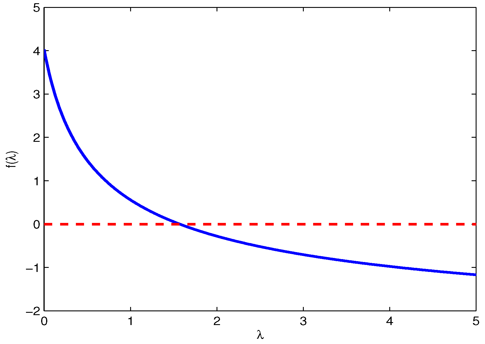
Proposition 3 suggests that f is monotonically decreasing over the non-negative real numbers. Moreover, we can choose a $\overline{\lambda }>0$ such that $f\left(\lambda \right)<0,\forall \lambda \in [\overline{\lambda },\infty )$. Let $\tilde{\lambda }\in [\overline{\lambda },\infty )$. Then, $f\left(\lambda \right)$ is a monotonically decreasing over $\lambda \in [0,\tilde{\lambda }]$, which connects $f\left(\tilde{\lambda }\right)<0$ and $f\left(0\right)>0$. The graph of f is illustrated in the following example.

Example 2. 

Let us consider Example 1 again. With $\gamma =3$ and $N=10$, the function value $f\left(\lambda \right)$ is plotted in Figure 1, demonstrating the monotonically non-increasing property and the zero crossing property in Proposition 3.

Based on Proposition 3, we can characterize the set of the KKT points. In particular, it turns out that the KKT point corresponding to $\lambda$ should satisfy the constraint $C\left({\left\{S_k^{\lambda }\right\}}_{k=0}^{N-1}\right)=\gamma$·

Proposition 4. 

The set of variables satisfying the KKT condition is all tuples ${(\lambda ,S_k^{\lambda },F_k^{\lambda },P_k^{\lambda })}_{k=0}^{N-1}$ such that $\lambda >0$ and $C\left({\left\{S_k^{\lambda }\right\}}_{k=0}^{N-1}\right)=\gamma$.

Proof. 

If $C\left({\left\{S_k^{\lambda }\right\}}_{k=0}^{N-1}\right)>\gamma$, the KKT condition is obviously not satisfied because the complementary slackness condition (5) is not satisfied with $\lambda >0$. If $C\left({\left\{S_k^{\lambda }\right\}}_{k=0}^{N-1}\right)<\gamma$, then the complementary slackness condition is not satisfied with $\lambda >0$. Only the case that KKT is satisfied with $\lambda >0$ is the case that $C\left({\left\{S_k^{\lambda }\right\}}_{k=0}^{N-1}\right)=\gamma$ holds. This completes the proof.    □

Proposition 4 gives us a clue on how to decide the KKT point. However, since the KKT condition is a necessary condition for the optimality, there is no guarantee that a KKT point found is actually an optimal solution. Fortunately, we can prove that all the KKT points characterized in Proposition 4 constitute the optimal solutions.

Proposition 5. 

Consider any tuples ${(\lambda ,S_k^{\lambda },F_k^{\lambda },P_k^{\lambda })}_{k=0}^{N-1}$ such that $\lambda >0$ and $C\left({\left\{S_k^{\lambda }\right\}}_{k=0}^{N-1}\right)=\gamma$. The set of such tuples is formally defined as

$$\Lambda :=\{{(\lambda ,S_k^{\lambda },F_k^{\lambda },P_k^{\lambda })}_{k=0}^{N-1}:\lambda >0,C\left({\left\{S_k^{\lambda }\right\}}_{k=0}^{N-1}\right)=\gamma \}$$

Then, the corresponding ${\left\{(S_k^{\lambda },F_k^{\lambda })\right\}}_{k=0}^{N-1}$ with ${(\lambda ,S_k^{\lambda },F_k^{\lambda },P_k^{\lambda })}_{k=0}^{N-1}\in \Lambda$ is an optimal solution of the constrained LQG problem in Problem 2.

Proof. 

From Proposition 4, we conclude that $\Lambda$ is the set of all KKT points. Therefore, there exists at least one ${({\lambda }^{\ast },S_k^{{\lambda }^{\ast }},F_k^{{\lambda }^{\ast }},P_k^{{\lambda }^{\ast }})}_{k=0}^{N-1}\in \Lambda$ such that the corresponding ${\left\{(S_k^{\lambda },F_k^{\lambda })\right\}}_{k=0}^{N-1}$ is an optimal solution of the constrained LQG problem in Problem 2. From statement 3) of Proposition 3, other elements in $\Lambda$ have the same objective function value $J_p\left({\left\{S_k^{\lambda }\right\}}_{k=0}^{N-1}\right)$. Therefore, for all ${(\lambda ,S_k^{\lambda },F_k^{\lambda },P_k^{\lambda })}_{k=0}^{N-1}\in \Lambda$, the corresponding ${\left\{(S_k^{\lambda },F_k^{\lambda })\right\}}_{k=0}^{N-1}$ is an optimal solution of the constrained LQG problem in Problem 2. This completes the proof.    □

Proposition 5 tells us that if we can find a root $\lambda >0$ satisfying $f\left(\lambda \right)=0$, then we can find an optimal solution of Problem 2. Therefore, the problem is reduced to finding a root of $f\left(\lambda \right)=0$. Our next goal is to develop a simple algorithm to solve the multi-objective LQG problem.

3.2. Algorithm

A natural way is to perform a line search over $\lambda \ge 0$ until $C\left({\left\{S_k^{\lambda }\right\}}_{k=0}^{N-1}\right)=\gamma$ holds. For instance, we can gradually increase $\lambda$ from 0 with a certain step size $\Delta \lambda >0$ until $f\left(\lambda \right)=0$ holds. Another way is to perform a bisection line search over a certain interval $\lambda \in [0,\overline{\lambda }],\overline{\lambda }>0$ and find a root $\lambda >0$ satisfying $f\left(\lambda \right)=0$. In this paper, we adopt the bisection search summarized in Algorithm 1. Note that the bisection search is valid because f is monotone in its argument, which is reduced to the monotonicity of $C\left({\left\{S_k^{\lambda }\right\}}_{k=0}^{N-1}\right)$. Moreover, Algorithm 1 can be seen as a primal-dual method because they alternate the primal and dual variables updates to estimate f. In Algorithm 1, f can be computed using Algorithm 2.

Algorithm 1 Primal-Dual Method with Bisection Line Search.

1: Input: accuracy $\epsilon >0$, line search interval $\tilde{\lambda }>0$ 2: Compute $f\left(0\right)=\mathrm{Eval}\left(0\right)$. 3: if  $f\left(0\right)\le 0$  then 4:     Stop and output 0. 5: end if 6: Let $a=0$ and $b=\tilde{\lambda }$. 7: for  $k\in \{0,1,\dots \}$  do 8:     Compute $f\left(a\right)=\mathrm{Eval}\left(a\right)$, $f\left(b\right)=\mathrm{Eval}\left(b\right)$, $c=(a+b)/2$, and $f\left(c\right)=\mathrm{Eval}\left(c\right)$ 9:     if $\left|\right(b-a)/2|\le \epsilon$ then 10:         Stop and output c 11:     end if 12:     if $\mathrm{sign}\left(f\right(c\left)\right)=\mathrm{sign}\left(f\right(a\left)\right)$ then 13:         $a\leftarrow c$ 14:     else 15:         $b\leftarrow c$ 16:     end if 17: end for

Algorithm 2 Policy evaluation $f\left(\lambda \right)=\mathrm{Eval}\left(\lambda \right)$.

1: Input: $\lambda$ 2: Dual update: Perform the recursion (Riccati equation) $$\begin{array}{c}\hfill A^T{X}_{k+1}^{\lambda }A-A^T{X}_{k+1}^{\lambda }B{(R_k+\lambda {\tilde{R}}_k+B^T{X}_{k+1}^{\lambda }B)}^{-1}{B}^T{X}_{k+1}^{\lambda }A+Q_k+\lambda {\tilde{Q}}_k=X_k^{\lambda }\end{array}$$ for all $k\in \{0,\dots ,N-1\}$ with $X_N^{\lambda }=Q_f+\lambda {\tilde{Q}}_f$. 3: Primal update: Compute the feedback gains $$\begin{array}{cc}\hfill F_k=& -{(R_k+\lambda {\tilde{R}}_k+B^T{X}_{k+1}B)}^{-1}{B}^T{X}_{k+1}A,k\in \{0,\dots ,N-1\}\hfill \end{array}$$ 4: Primal update: Perform the recursion $$\begin{array}{cc}\hfill & \Phi (F_k,S_{k-1})=S_k,k\in \{1,\dots ,N-1\},\hfill \end{array}$$ with $\left[\begin{array}{c}{I}_n\\ F_0\end{array}\right](V+z{z}^T){\left[\begin{array}{c}{I}_n\\ F_0\end{array}\right]}^T=S_0$. 5: Compute $$\begin{array}{cc}\hfill {\tilde{J}}_p\left({\left\{S_k^{\lambda }\right\}}_{k=0}^{N-1}\right):=& Tr\left({\tilde{Q}}_f\left({\left[\begin{array}{c}{A}^T\\ B^T\end{array}\right]}^T{S}_{N-1}^{\lambda }\left[\begin{array}{c}{A}^T\\ B^T\end{array}\right]+W\right)\right)+\sum _{k=0}^{N-1}Tr\left(\left[\begin{array}{cc}{\tilde{Q}}_k& 0\\ 0& {\tilde{R}}_k\end{array}\right]S_k^{\lambda }\right)\hfill \end{array}$$ 6: Output: $f\left(\lambda \right)={\tilde{J}}_p\left({\left\{S_k^{\lambda }\right\}}_{k=0}^{N-1}\right)-\gamma$

3.3. Suboptimality

Once an approximate $\lambda$ is found from Algorithm 1, the corresponding solution ${\{S_k^{\lambda },P_k^{\lambda },F_k^{\lambda }\}}_{k=0}^{N-1}$ can be easily found. The solution obtained by Algorithm 1 is $\epsilon$-accurate in terms of $\lambda$, while it does not guarantee the $\epsilon$-accuracy in terms of the objective $f\left(\lambda \right)$ or other variables ${\{S_k^{\lambda },P_k^{\lambda },F_k^{\lambda }\}}_{k=0}^{N-1}$ induced from the $\epsilon$-accuracy of $\lambda$, which depend on their sensitivities in $\lambda$. From the structures of $f\left(\lambda \right)$ or ${\{S_k^{\lambda },P_k^{\lambda },F_k^{\lambda }\}}_{k=0}^{N-1}$, we can conclude that if $\lambda$ is $\epsilon$-accurate, then $f\left(\lambda \right)$ is $\rho \left(\epsilon \right)$-accurate, i.e., $\left|f\right(\lambda \left)\right|\le \rho \left(\epsilon \right)$ for some function $\rho$ such that $\rho \left(\epsilon \right)\to 0$ as $\epsilon \to 0$. The function $\rho$ depends on the system parameters such as $(A,B)$, $Q_f,Q_k,R_k,{\tilde{Q}}_f,{\tilde{Q}}_k,{\tilde{R}}_k,k\ge 0$, and N.

Due to the finite precision error in the bisection search, it is hard to satisfy the equality $C({\left\{S_k^{\lambda }\right\}}_{k=0}^{N-1})=\gamma$ or $f\left(\lambda \right)=0$ exactly. Assume that $f\left(\lambda \right)$ is $\rho$-accurate, i.e., $\left|f\right(\lambda \left)\right|\le \rho$. This implies

$$C\left({\left\{S_k^{\lambda }\right\}}_{k=0}^{N-1}\right)-\gamma =:a\in (-\rho ,\rho )$$

Then, such $\lambda >0$ is the dual variable such that

$$C\left({\left\{S_k^{\lambda }\right\}}_{k=0}^{N-1}\right)=\gamma +a$$

is satisfied, and the corresponding tuple ${\{\lambda ,S_k^{\lambda },P_k^{\lambda },F_k^{\lambda }\}}_{k=0}^{N-1}$ satisfies the KKT condition with $\gamma \leftarrow \gamma +a$. We can conclude that ${\{S_k^{\lambda },F_k^{\lambda }\}}_{k=0}^{N-1}$ is an optimal solution of Problem 2 with $\gamma$ replaced with $\gamma +a\in (\gamma -\rho ,\gamma +\rho )$.

Proposition 6. 

Suppose that given $\lambda >0$, $f\left(\lambda \right)$ is ρ-accurate, i.e., $\left|f\right(\lambda \left)\right|\le \rho$, and define

$$C\left({\left\{S_k^{\lambda }\right\}}_{k=0}^{N-1}\right)-\gamma =:a\in (-\rho ,\rho )$$

Then, for the corresponding tuple ${\{\lambda ,S_k^{\lambda },P_k^{\lambda },F_k^{\lambda }\}}_{k=0}^{N-1}$, ${\{S_k^{\lambda },F_k^{\lambda }\}}_{k=0}^{N-1}$ is an optimal solution of Problem 2 with γ replaced with $\gamma +a\in (\gamma -\rho ,\gamma +\rho )$.

Proof. 

The corresponding tuple ${\{\lambda ,S_k^{\lambda },P_k^{\lambda },F_k^{\lambda }\}}_{k=0}^{N-1}$ satisfies the KKT condition with the complement slackness condition replaced with $\lambda ({\tilde{J}}_p\left({\left\{S_k\right\}}_{k=0}^{N-1}\right)-\gamma -a)=0$. The proof is concluded using Proposition 5. □

Proposition 6 suggests that the solution obtained by using Algorithm 1 is a suboptimal solution of Problem 2 with $\gamma$ replaced with $\gamma +a$.

3.4. Computational Efficiency

The number of variables in the problem is upper bounded by $O(n^2·N)$. If we use an SDP to solve the multi-objective problem using interior point algorithms, the time complexity is known to be upper bounded by $O(n^6·N^3·log(1/\epsilon ))$ to obtain an $\epsilon$-accurate solution [33]. Therefore, the computational time may explode cubically as $N\to \infty$. On the other hand, the bisection line search is known to find an $\epsilon$-accurate solution within the number of iterations bounded by $O(log({\epsilon }_0/\epsilon ))$, where ${\epsilon }_0=|b-a|$ is the initial bracket size. The time complexity of the proposed algorithm per iteration is $O(n^2·N)$. Therefore, the overall time complexity is bounded by $O(n^2·N·log({\epsilon }_0/\epsilon ))$, which is linear in N. Assuming that both notions of the $\epsilon$-accuracy is reasonably compatible for fair comparisons, the proposed bisection algorithm may perform much faster than the interior-point algorithms, especially when N is large, which is the case in most applications. In particular, when the model predictive control is applied, where Problem 2 is solved at every iteration, the proposed scheme could play an important role. The compatibility of the $\epsilon$-accuracy of both approaches is hard to address within the scope of this paper. We will provide a numerical comparative analysis at the end of this paper to demonstrate the efficiency of the algorithm.

3.5. Deterministic Cases

The previous results assume that the noises are stochastic and the covariance matrices V and W are positive definite. However, it does not cover important applications where some variables are deterministic or fixed. To cover more practical cases, we will extend the results to the generic case that some elements of the noise vectors are deterministic. In this case, $V\succ 0,W\succ 0$ should be relaxed to $V⪰0,W⪰0$. Note that if $V\succ 0,W\succ 0$, then the KKT point in Proposition 1 uniquely satisfies the KKT condition for any fixed $\lambda >0$. For the deterministic case $V=W=0$ or $V⪰,W⪰0$, it still satisfies the KKT condition, while it may not be a unique solution. Therefore, we cannot preserve the optimality arguments in Proposition 5. Fortunately, the previous results hold in this case under mild assumptions.

Proposition 7. 

Suppose that the second condition, $V\succ 0,W\succ 0$, in Assumption 1 is relaxed to $V⪰0,W⪰0$. Assume that f is a bijection for the given $V⪰0,W⪰0$. Consider any tuples ${(\lambda ,S_k^{\lambda },F_k^{\lambda },P_k^{\lambda })}_{k=0}^{N-1}$ such that $\lambda >0$ and $C\left({\left\{S_k^{\lambda }\right\}}_{k=0}^{N-1}\right)=\gamma$. Then, the corresponding ${\left\{(S_k^{\lambda },F_k^{\lambda })\right\}}_{k=0}^{N-1}$ is an optimal solution of the constrained LQG problem in Problem 2.

Proof. 

We first prove the continuity of ${(\lambda ,S_k^{\lambda },F_k^{\lambda },P_k^{\lambda })}_{k=0}^{N-1}$ as a function of V and W, and denote them by ${(\lambda ,S_k^{\lambda ,V,W},F_k^{\lambda ,V,W},P_k^{\lambda ,V,W})}_{k=0}^{N-1}$. First of all, suppose that $\lambda >0$ is fixed. Then, $F_k^{\lambda ,V,W}$ and $P_k^{\lambda ,V,W}$ do not depend on V and W, and hence are continuous as functions of $(V,W)$. Moreover, $S_k^{\lambda ,V,W}$ depends on $(V,W)$ linearly, and thus, is continuous in $(V,W)$. Similarly, so are $J_p^{V,W}$ and $C^{V,W}$ as functions of $(V,W)$. Now, $f^{V,W}$ is also continuous as a function of $(V,W)$ and $\lambda$. Consider the set-valued mapping $T:(V,W)\mapsto \{\lambda >0:f^{V,W}\left(\lambda \right)=0\}$. If f is bijective for $V⪰0$ and $W⪰0$, then the output of T is singleton, and $T(V,W)$ is the point on the graph of $f^{V,W}$, which crosses zero because the Lagrange multiplier ${\lambda }^{\ast }>0$, which solves the KKT condition as a root of $f^{V,W}\left(\lambda \right)$. Therefore, from the continuity of $f^{V,W}$ on $(V,W)$ and $\lambda \ge 0$, we can prove that $T:{\mathbb{R}}^{n\times n}\times {\mathbb{R}}^{m\times m}\to {\mathbb{R}}_{++}$ is also continuous as follows. First of all, note that by the continuity of $f^{V,W}$ on $(V,W)$, $f^{V,W}$ is a bijection for all $(V^{\prime },W^{\prime })$ around $(V,W)$. In the sequel, assume that $(V^{\prime },W^{\prime })$ always lies inside such a set. Note also that $T(V,W)={\left(f^{V,W}\right)}^{-1}\left(0\right)$ and ${\left(f^{V,W}\right)}^{-1}\left(y\right)$ is continuous in y by the continuity of $f^{V,W}\left(\lambda \right)$ in $\lambda$. We will show that for any $\epsilon >0$, there exists $\delta >0$ such that ${∥V-V^{\prime }∥}_2+{∥W-W^{\prime }∥}_2<\delta$ implies $|T(V,W)-T(V^{\prime },W^{\prime })|<\epsilon$. To proceed, let us define $T(V,W)={\left(f^{V,W}\right)}^{-1}\left(0\right)={\lambda }^{\ast }$ and $T(V^{\prime },W^{\prime })={\left(f^{V^{\prime },W^{\prime }}\right)}^{-1}\left(0\right)={\lambda }^{\prime }$. By the continuity of $f^{V,W}$ in V and W, for any ${\epsilon }^{\prime }>0$, there exists $\delta >0$ such that ${∥V-V^{\prime }∥}_2+{∥W-W^{\prime }∥}_2<\delta$ implies $|f^{V,W}\left({\lambda }^{\ast }\right)-f^{V^{\prime },W^{\prime }}\left({\lambda }^{\ast }\right)|<{\epsilon }^{\prime }$. Moreover, by the continuity of ${\left(f^{V,W}\right)}^{-1}\left(y\right)$ in y, for any $\epsilon >0$, there exists ${\epsilon }^{\prime }>0$ such that $|x-y|<{\epsilon }^{\prime }$ implies $|{\left(f^{V^{\prime },W^{\prime }}\right)}^{-1}\left(x\right)-{\left(f^{V^{\prime },W^{\prime }}\right)}^{-1}\left(y\right)|<\epsilon$. With $x=f^{V,W}\left({\lambda }^{\ast }\right),y=f^{V^{\prime },W^{\prime }}\left({\lambda }^{\ast }\right)$, we have

$$\begin{array}{cc}\hfill & |{\left(f^{V^{\prime },W^{\prime }}\right)}^{-1}\left(f^{V,W}\left({\lambda }^{\ast }\right)\right)-{\left(f^{V^{\prime },W^{\prime }}\right)}^{-1}\left(f^{V^{\prime },W^{\prime }}\left({\lambda }^{\ast }\right)\right)|\hfill \\ \hfill =& |{\left(f^{V^{\prime },W^{\prime }}\right)}^{-1}\left(0\right)-{\lambda }^{\ast }|\hfill \\ \hfill =& |{\left(f^{V^{\prime },W^{\prime }}\right)}^{-1}\left(0\right)-{\left(f^{V,W}\right)}^{-1}\left(0\right)|\hfill \\ \hfill <& \epsilon \hfill \end{array}$$

Therefore, this proves the continuity of $T(V,W)={\left(f^{V,W}\right)}^{-1}\left(0\right)$ in V and W. Hence, ${(\lambda ,S_k^{\lambda ,V,W},F_k^{\lambda ,V,W},P_k^{\lambda ,V,W})}_{k=0}^{N-1}$ is continuous as a function of V and W. Note that $\lambda$ is also a function of $(V,W)$. As the next step, consider a sequence ${(V_i,W_i)}_{i=0}^{\infty }$ such that $V_i=V+{\left(0.5\right)}^{i}I$ and $W_i=W+{\left(0.5\right)}^{i}I$ so that $(V_i,W_i)\to (V,W)$ as $i\to \infty$ and $V_i\succ 0,W_i\succ 0$ for all $i\ge 0$. Then, the corresponding ${(S_k^{{\lambda }_i,V_i,W_i},F_k^{{\lambda }_i,V_i,W_i})}_{k=0}^{N-1}$ is the unique optimal solution corresponding to $V_i$ and $W_i$, where ${\lambda }_i$ is the Lagrange multiplier corresponding to $V_i$ and $W_i$. From the continuity of the KKT point in $(V,W)$, we can arrive at the desired conclusion. □

3.6. Example

In this section, we will provide a simple example to illustrate the validity and efficiency of the proposed approach. The numerical example was treated with the help of MATLAB R2020a. The SDPs were solved with SeDuMi [34] and Yalmip [35]. Let us consider Example 1 again with the following setting:

$$N=1000,\gamma =\mathrm{25,000},V=0,W=0.01I,z=\left[\begin{array}{c}25\\ 25\\ 30\\ 24\end{array}\right]$$

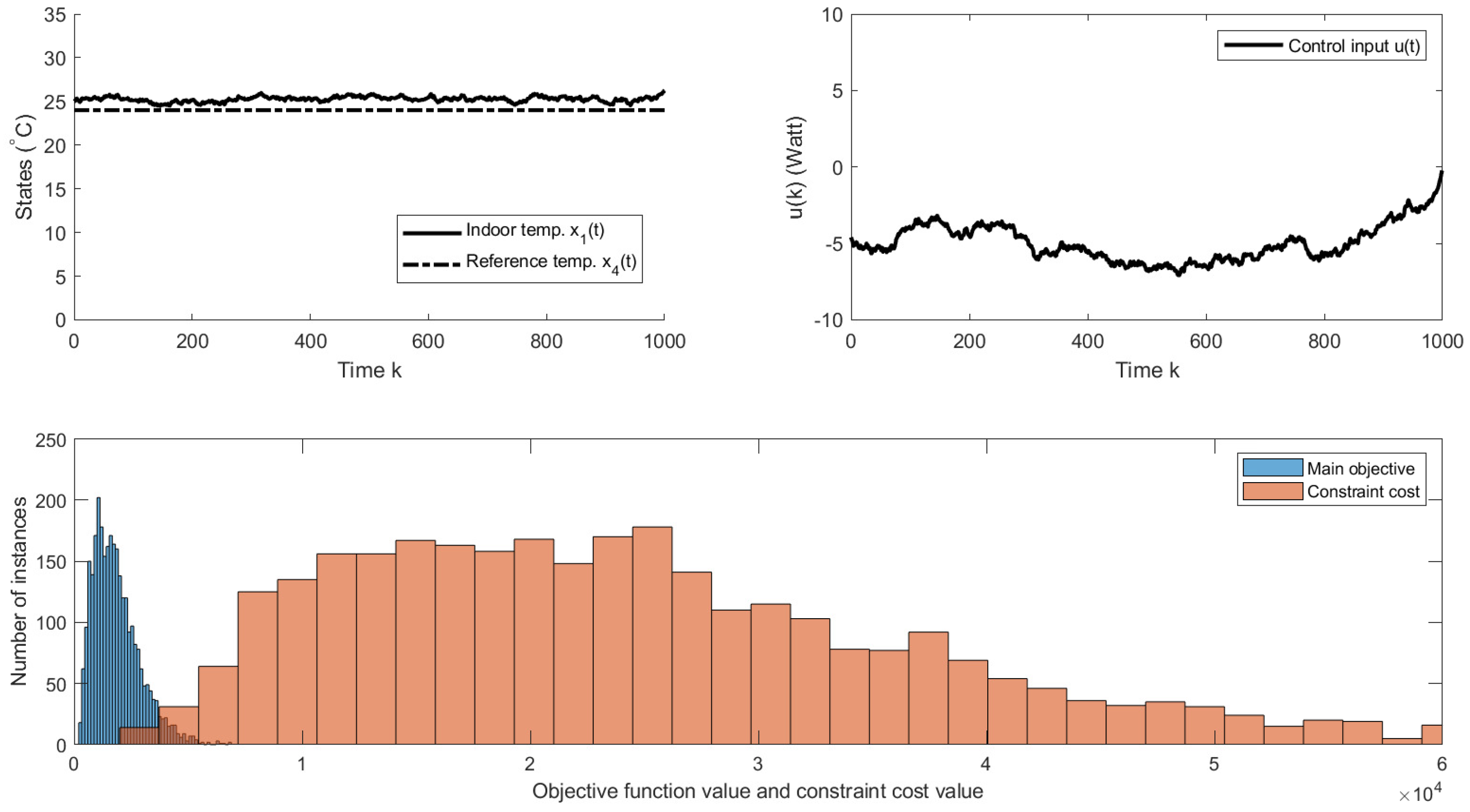
Running the proposed algorithm with the initial search interval $[0,\tilde{\lambda }]=[0,100]$ and the accuracy $\epsilon =0.000001$ leads to ${\lambda }^{\ast }=0.2448$ with the elapsed time $1.83$ seconds. With the obtained control policy, the evolution of the indoor temperature $x_1\left(t\right)$ (${}^{\circ }$C), reference temperature $x_4\left(t\right)$ (${}^{\circ }$C), input $u\left(t\right)$ (${}^{\circ }$C), and the histograms of the objective function and constraint cost are depicted in Figure 2. The histogram has been obtained over 3000 samples, and the empirical average of the constraint cost is 25,129, which meets the inequality constraint approximately.

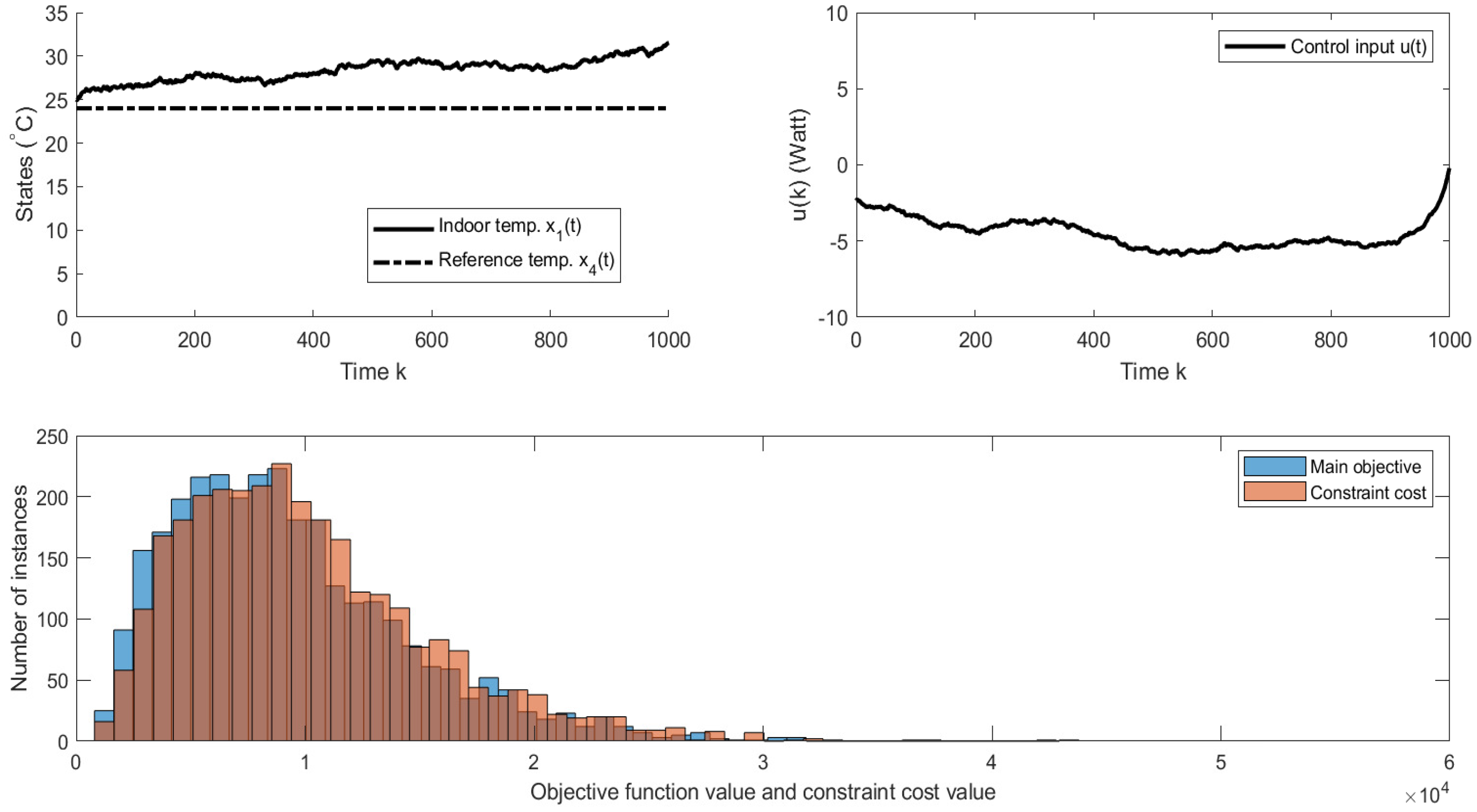
Running the proposed algorithm with the same setting except for $\gamma$ = 10,000 leads to ${\lambda }^{\ast }=0.8959$. The corresponding simulation results are given in Figure 3. The empirical average of the constraint cost from samples in histogram is 9956, which meets the inequality constraint approximately.

A semidefinite programming problem (SDP) for solving the same problem, Problem 2 is given by

$$\begin{array}{cc}\hfill & \underset{S_k,k\in \{0,1,\dots ,N\},\lambda \ge 0}{max}\sum _{k=0}^{N}Tr{S}_k-\lambda \gamma \hfill \\ \hfill & \mathrm{subject}\mathrm{to}\hfill \\ \hfill & \left[\begin{array}{cc}{Q}_k+\lambda {\tilde{Q}}_k& 0\\ 0& R_k+\lambda {\tilde{R}}_k\end{array}\right]+\left[\begin{array}{cc}{A}^T{S}_{k+1}A-S_k& A^T{S}_{k+1}B\\ B^T{S}_{k+1}A& B^T{S}_{k+1}B\end{array}\right]⪰0,k\in \{0,1,\dots ,N\}\hfill \end{array}$$

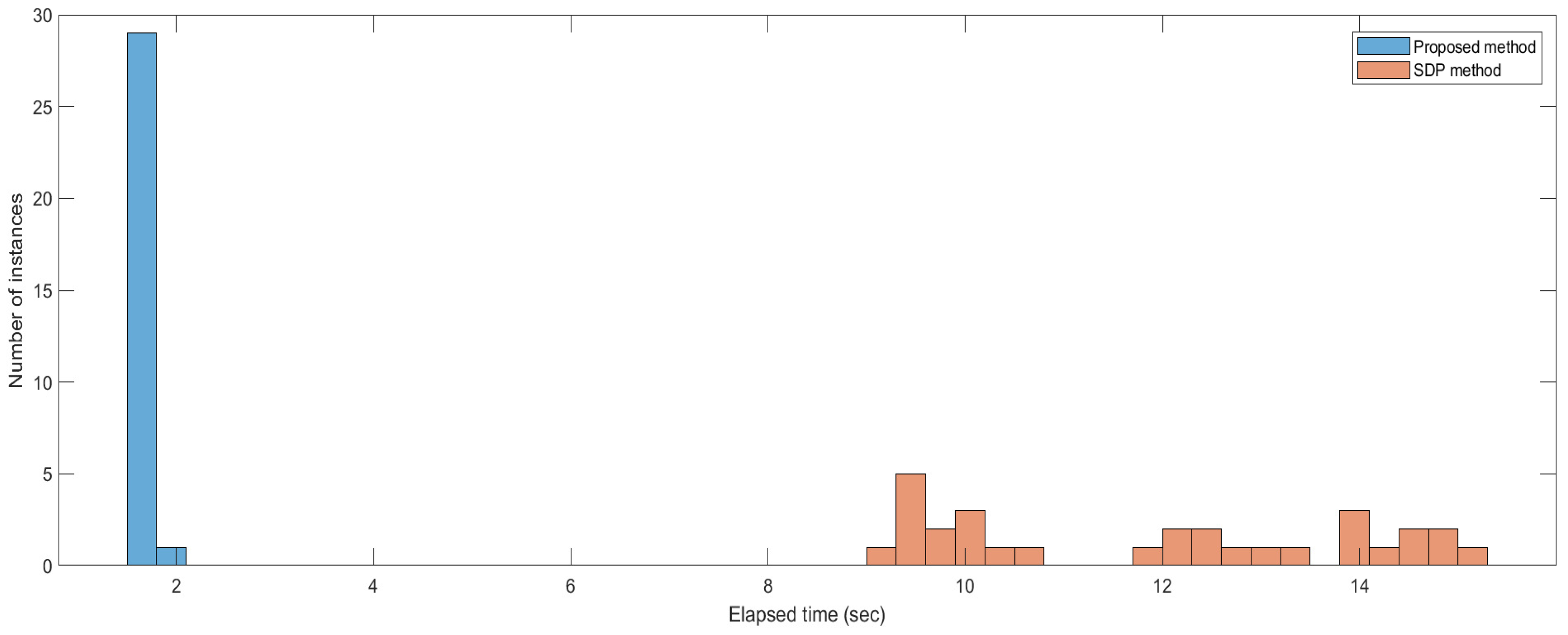
with $S_{N+1}=0,Q_N=Q_f,{\tilde{Q}}_N={\tilde{Q}}_f,R_N={\tilde{R}}_N=0$, which can be readily obtained by modifying the results in [29]. The histograms of the elapsed times of the proposed algorithm and the above SDP problem to solve the building problem are shown in Figure 4 over 30 samples.

The average elapsed times are $1.7551$ s and $11.8987$ s for the proposed method and the SDP problem, respectively. The result demonstrates that the proposed algorithm is computationally more efficient than the SDP approach.

4. Conclusions

In this paper, we have studied a multi-objective linear quadratic Gaussian (LQG) control problem subject to an input energy constraint. To solve this problem efficiently, we have proposed a bisection line search algorithm based on optimization and Lagrangian theories. Our approach has been thoroughly investigated by analyzing optimal solutions using the Karush–Kuhn–Tucker (KKT) condition, and we have proven the convergence guarantees of the algorithm. We have also demonstrated the applicability and efficiency of the proposed algorithm by applying it to a building control problem.

The proposed algorithm has the potential to be applied to fast model predictive control and to provide new insights into LQG problems. However, we acknowledge that the bisection line search algorithm may become inefficient in multi-constraint scenarios due to the high-dimensional search space. Hence, in future work, we aim to investigate and develop new algorithms that can efficiently handle problems with multiple constraints.

References

- Bertsekas, D.P.; Tsitsiklis, J.N. Neuro-Dynamic Programming; Athena Scientific: Belmont, MA, USA, 1996. [Google Scholar]
- Bertsekas, D.P. Dynamic Programming and Optimal Control, 3rd ed.; Athena Scientific: Nashua, MA, USA, 2005; Volume 1. [Google Scholar]
- Lee, D. Convergence of Dynamic Programming on the Semidefinite Cone for Discrete-Time Infinite-Horizon LQR. IEEE Trans. Autom. Control 2022, 67, 5661–5668. [Google Scholar] [CrossRef]
- Sabermahani, S.; Ordokhani, Y. Fibonacci wavelets and Galerkin method to investigate fractional optimal control problems with bibliometric analysis. J. Vib. Control 2021, 27, 1778–1792. [Google Scholar] [CrossRef]
- Boyd, S.; Vandenberghe, L. Convex Optimization; Cambridge University Press: Cambridge, UK, 2004. [Google Scholar]
- Vandenberghe, L.; Boyd, S. Semidefinite programming. SIAM Rev. 1996, 38, 49–95. [Google Scholar] [CrossRef] [Green Version]
- Boyd, S.; El Ghaoui, L.; Feron, E.; Balakrishnan, V. Linear Matrix Inequalities in Systems and Control Theory; SIAM: Philadelphia, PA, USA, 1994. [Google Scholar]
- El Ghaoui, L.; Niculescu, S.I. Advances in Linear Matrix Inequality Methods in Control; SIAM: University City, PA, USA, 2000; Volume 2. [Google Scholar]
- Scherer, C.; Weiland, S. Linear Matrix Inequalities in Control; Lecture Notes; Dutch Institute for Systems and Control: Delft, The Netherlands, 2000; Volume 3. [Google Scholar]
- Lee, D.H.; Park, J.B.; Joo, Y.H. A less conservative LMI condition for robust D-stability of polynomial matrix polytopes—A projection approach. IEEE Trans. Autom. Control 2010, 56, 868–873. [Google Scholar] [CrossRef]
- Lee, D.H.; Joo, Y.H. A note on sampled-data stabilization of LTI systems with aperiodic sampling. IEEE Trans. Autom. Control 2015, 60, 2746–2751. [Google Scholar] [CrossRef]
- Cao, Y.Y.; Lin, Z. A descriptor system approach to robust stability analysis and controller synthesis. IEEE Trans. Autom. Control 2004, 49, 2081–2084. [Google Scholar] [CrossRef]
- Oliveira, R.C.; Peres, P.L. Parameter-dependent LMIs in robust analysis: Characterization of homogeneous polynomially parameter-dependent solutions via LMI relaxations. IEEE Trans. Autom. Control 2007, 52, 1334–1340. [Google Scholar] [CrossRef]
- Ramos, D.C.; Peres, P.L. An LMI condition for the robust stability of uncertain continuous-time linear systems. IEEE Trans. Autom. Control 2002, 47, 675–678. [Google Scholar] [CrossRef]
- Chesi, G.; Garulli, A.; Tesi, A.; Vicino, A. Polynomially parameter-dependent Lyapunov functions for robust stability of polytopic systems: An LMI approach. IEEE Trans. Autom. Control 2005, 50, 365–370. [Google Scholar] [CrossRef]
- Fridman, E.; Shaked, U. Parameter dependent stability and stabilization of uncertain time-delay systems. IEEE Trans. Autom. Control 2003, 48, 861–866. [Google Scholar] [CrossRef]
- Yan, S.; Shen, M.; Nguang, S.K.; Zhang, G. Event-triggered H∞ control of networked control systems with distributed transmission delay. IEEE Trans. Autom. Control 2019, 65, 4295–4301. [Google Scholar] [CrossRef]
- Felipe, A.; Oliveira, R.C. An LMI-based algorithm to compute robust stabilizing feedback gains directly as optimization variables. IEEE Trans. Autom. Control 2020, 66, 4365–4370. [Google Scholar] [CrossRef]
- Guo, M.; De Persis, C.; Tesi, P. Data-driven stabilization of nonlinear polynomial systems with noisy data. IEEE Trans. Autom. Control 2021, 67, 4210–4217. [Google Scholar] [CrossRef]
- Lee, D.; Lee, S.; Karava, P.; Hu, J. Simulation-based policy gradient and its building control application. In Proceedings of the 2018 Annual American Control Conference (ACC), Milwaukee, WI, USA, 27–29 June 2018; pp. 5424–5429. [Google Scholar]
- Ma, Y.; Borrelli, F. Fast stochastic predictive control for building temperature regulation. In Proceedings of the 2012 American Control Conference (ACC), Montreal, QC, Canada, 27–29 June 2012; pp. 3075–3080. [Google Scholar]
- Oldewurtel, F.; Parisio, A.; Jones, C.N.; Morari, M.; Gyalistras, D.; Gwerder, M.; Stauch, V.; Lehmann, B.; Wirth, K. Energy efficient building climate control using stochastic model predictive control and weather predictions. In Proceedings of the 2010 American Control Conference, Baltimore, ML, USA, 30 June–2 July 2010; pp. 5100–5105. [Google Scholar]
- Luenberger, D.G.; Ye, Y. Linear and Nonlinear Programming; Addison-Wesley: Reading, MA, USA, 1984; Volume 2. [Google Scholar]
- Bemporad, A.; Morari, M.; Dua, V.; Pistikopoulos, E.N. The explicit linear quadratic regulator for constrained systems. Automatica 2002, 38, 3–20. [Google Scholar] [CrossRef]
- Grieder, P.; Borrelli, F.; Torrisi, F.; Morari, M. Computation of the constrained infinite time linear quadratic regulator. Automatica 2004, 40, 701–708. [Google Scholar] [CrossRef]
- Borrelli, F. Constrained Optimal Control of Linear and Hybrid Systems; Springer: Berlin/Heidelberg, Germany, 2003; Volume 290. [Google Scholar]
- Chisci, L.; Zappa, G. Fast algorithm for a constrained infinite horizon LQ problem. Int. J. Control 1999, 72, 1020–1026. [Google Scholar] [CrossRef]
- Rotea, M.A. The generalized H2 control problem. Automatica 1993, 29, 373–385. [Google Scholar] [CrossRef]
- Gattami, A. Generalized linear quadratic control. IEEE Trans. Autom. Control 2010, 55, 131–136. [Google Scholar] [CrossRef]
- Kothare, M.V.; Balakrishnan, V.; Morari, M. Robust constrained model predictive control using linear matrix inequalities. Automatica 1996, 32, 1361–1379. [Google Scholar] [CrossRef] [Green Version]
- Primbs, J.A.; Sung, C.H. Stochastic receding horizon control of constrained linear systems with state and control multiplicative noise. IEEE Trans. Autom. Control 2009, 54, 221–230. [Google Scholar] [CrossRef]
- Costa, O.L.V.; Assumpção Filho, E.; Boukas, E.; Marques, R. Constrained quadratic state feedback control of discrete-time Markovian jump linear systems. Automatica 1999, 35, 617–626. [Google Scholar] [CrossRef]
- Gahinet, P.; Nemirovski, A.; Laub, A.J.; Chilali, M. LMI Control Toolbox; The Math Works Inc.: Natick, MA, USA, 1996. [Google Scholar]
- Sturm, J.F. Using SeDuMi 1.02, a MATLAB toolbox for optimization over symmetric cones. Optim. Methods Softw. 1999, 11, 625–653. [Google Scholar] [CrossRef]
- Lofberg, J. YALMIP: A toolbox for modeling and optimization in MATLAB. In Proceedings of the 2004 IEEE International Conference on Robotics and Automation (IEEE Cat. No. 04CH37508), New Orleans, LA, USA, 2–4 September 2004; pp. 284–289. [Google Scholar]
Figure 1.
for different .
Figure 2.
With , the top figures show evolution of the indoor temperature , reference temperature , and the input . The bottom figure depicts the histograms of the objective function and constraint cost.
Figure 3.
Figure 4.
The histograms of the elapsed times of the proposed algorithm and the SDP problem.
Disclaimer/Publisher’s Note: The statements, opinions and data contained in all publications are solely those of the individual author(s) and contributor(s) and not of MDPI and/or the editor(s). MDPI and/or the editor(s) disclaim responsibility for any injury to people or property resulting from any ideas, methods, instructions or products referred to in the content. |
© 2023 by the author. Licensee MDPI, Basel, Switzerland. This article is an open access article distributed under the terms and conditions of the Creative Commons Attribution (CC BY) license (https://creativecommons.org/licenses/by/4.0/).
Share and Cite
MDPI and ACS Style
Lee, D. Multi-Objective LQG Design with Primal-Dual Method. Mathematics 2023, 11, 1857. https://doi.org/10.3390/math11081857
AMA Style
Lee D. Multi-Objective LQG Design with Primal-Dual Method. Mathematics. 2023; 11(8):1857. https://doi.org/10.3390/math11081857
Chicago/Turabian StyleLee, Donghwan. 2023. "Multi-Objective LQG Design with Primal-Dual Method" Mathematics 11, no. 8: 1857. https://doi.org/10.3390/math11081857
Note that from the first issue of 2016, this journal uses article numbers instead of page numbers. See further details here.