A Second-Order Accurate Numerical Approximation for a Two-Sided Space-Fractional Diffusion Equation

Abstract

In this paper, we investigate a practical numerical method for solving a one-dimensional two-sided space-fractional diffusion equation with variable coefficients in a finite domain, which is based on the classical Crank-Nicolson (CN) method combined with Richardson extrapolation. Second-order exact numerical estimates in time and space are obtained. The unconditional stability and convergence of the method are tested. Two numerical examples are also presented and compared with the exact solution.

1. Introduction

In recent years, fractional differential equations have been of great interest for their use in modelling problems in physics (for an excellent review, see [1]), biology [2], chemistry [3] and even finance [4]. Numerical methods have become the main way to solve fractional-order equations, since we cannot easily obtain explicit analytical solutions to fractional-order equations. Several authors have proposed some effective numerical methods. Liu et al. [5] proposed a novel spatial second-order exact semi-implicit alternating direction method for the two-dimensional fractional FitzHugh-Nagumo single-domain model. Li et al. [6] proposed a spectral method for solving a fractional diffusion-absorption-reaction equation. She et al. [7] studied and analysed the Crank-Nicolson time discretisation of one- and two-dimensional spatial fractional diffusion equations. Hao et al. [8] studied the regularity of two-sided fractional diffusion equations with reaction terms and spectral methods. Li et al. [9] studied the fractional spectral localisation discretization of optimal control problems governed by spatial fractional diffusion equations. Gunzburger et al. [10] proposed a stable finite volume element method to approximate the coupled Stokes-Darcy problem. Ozbilge et al. [11] considered a finite difference scheme for the inverse problem of time-fractional parabolic partial differential equations with non-local boundary conditions. Feng et al. [12] developed a new fractional finite volume method based on the nodal basis functions for a two-sided space-fractional diffusion equation. Liu et al. [13] considered the problem of minimising a non-convex integral function in control, which is a solution to a control system described by fractional differential equations with mixed non-convex constraints on the control. Jia et al. [14] considered a fast finite difference method for a spatial fractional diffusion equation with fractional derivative boundary conditions. Lai et al. [15] considered the numerical solution of a Riesz spatial fractional partial differential equation with second order time derivatives. Chen et al. [16] considered a compact difference scheme for a second-order backward differential formulation of the fractional-order Volterra equation with a truncation error of order 4 in time and order 4 in space. Ma et al. [17] proposed a new signal smoothing equations, and they introduced generalized filters by use of memory effects of fractional derivatives. Shiri et al. [18] proposed an interesting Neural Network method for solving diffusion equations. Qu et al. [19] proposed a weight finite difference scheme for space fractional diffusion equations. There are some new papers in the fractional differential equations (see [20,21]). Based on the fractional-order Fick’s law, a fractional-order diffusion model is derived for the space of variable coefficients with two-sided derivatives in the conserved form. The continuum equation in one-dimensional form can be written according to the mass conservation law as

$$\frac{\partial p(x,t)}{\partial t}+\frac{\partial Q(x,t)}{\partial x}=f(x,t),$$

(1)

where $p(x,t)$ is the distribution function of the diffusing quantity, $Q(x,t)$ is the diffusion flux and $f(x,t)$ is the source term. The classical Fick’s law can be extended as follows:

$$Q(x,t)=-C\left(x\right)\frac{\partial }{\partial x}{\int }_a^x{K}_{+}(x,\xi )p(\xi ,t)d\xi -D\left(x\right)\frac{\partial }{\partial x}{\int }_x^b{K}_{-}(x,\xi )p(\xi ,t)d\xi ,$$

(2)

where $C\left(x\right)$ and $D\left(x\right)$ are non-negative diffusion coefficients. On the interval $[a,b]$, $C\left(x\right)$ is a monotonically decreasing function of x and $D\left(x\right)$ is a monotonically increasing function of x. The kernel functions $K_{+}(x,\xi )$ and $K_{-}(x,\xi )$ are defined as follows

$$\left\{\begin{array}{cc}{K}_{+}(x,\xi )=\frac{1}{\mathsf{\Gamma }(1-\alpha )}{(x-\xi )}^{-\alpha }\hfill & a\le \xi \le x,\hfill \\ K_{-}(x,\xi )=\frac{1}{\mathsf{\Gamma }(1-\alpha )}{(\xi -x)}^{-\alpha }\hfill & x\le \xi \le b,\hfill \end{array}\right.$$

(3)

where $0<\alpha <1$. Combination of Equations (1) and (2), Chen et al. [22] have derived the following nonlinear two-sided space fractional diffusion equation with variable coefficients.

$$\begin{gathered} \frac{\partial p(x,t)}{\partial t}=\frac{\partial }{\partial x}(C\left(x\right)\frac{{\partial }^{\alpha }p(x,t)}{\partial x^{\alpha }}-D\left(x\right)\frac{{\partial }^{\alpha }p(x,t)}{\partial {(-x)}^{\alpha }})+f(x,t), \\ a\le x\le b,0<\alpha <1,0<t\le T, \end{gathered}$$

(4)

where $\frac{{\partial }^{\alpha }p(x,t)}{{\partial }^{\alpha }(-x)}$ is the right Riemman-Liouville fractional derivatives, $\frac{{\partial }^{\alpha }p(x,t)}{{\partial }^{\alpha }x}$ is the left Riemman-Liouville fractional derivatives (see [23,24] for details) defined by

$$\frac{{\partial }^{\alpha }p(x,t)}{\partial {(-x)}^{\alpha }}=\frac{-1}{\mathsf{\Gamma }(1-\alpha )}\frac{\partial }{\partial x}{\int }_x^b\frac{p(s,t)}{{(s-x)}^{\alpha }}ds,$$

(5)

$$\frac{{\partial }^{\alpha }p(x,t)}{\partial x^{\alpha }}=\frac{1}{\mathsf{\Gamma }(1-\alpha )}\frac{\partial }{\partial x}{\int }_a^x\frac{p(s,t)}{{(x-s)}^{\alpha }}ds.$$

(6)

In this paper, we consider the above one-dimensional fractional two-sided space-fractional diffusion Equation (4) with the following initial value conditions and Dirichlet boundary conditions:

$$p(x,0)=\varphi \left(x\right),a\le x\le b,$$

(7)

$$p(a,t)=p(b,t)=0,0\le t\le T.$$

(8)

For this new one-dimensional two-sided spatial fractional diffusion equation, Chen et al. [22] gave a fast semi-implicit difference method. However, the method is only first order accuracy. To the best of our knowledge, there is limited research on the numerical computation of this equation with high accuracy based on the classical Crank-Nicolson scheme. This motivates us to propose in this paper an approach to this equation based on the classical Crank-Nicolson scheme and combined with a Richard space extrapolation. Our method is second order accuracy in time and space.

The remaining work is structured as follows. In Section 2, we present the classical Crank-Nicolson difference method for the one-dimensional two-sided spatial fractional diffusion equation and analyse its consistency. In Section 3, we prove the stability and convergence of the method. The method is then combined with spatial extrapolation. The convergence accuracy is improved to second order accuracy in time and space. In Section 4, two numerical experiments are given in order to verify the theoretical analysis of the method.

2. The Classical CN Difference Scheme for the One-Dimensional Two-Sided Space-Fractional Diffusion Equation and Its Consistency

For the numerical approximation, define $t_n=n\Delta t$, $0\le t_n\le T$, for $n=0,1,2,\dots ,N$ and $x_i=a+ih$ for $i=0,1,\dots ,M$, where $\Delta t,h$ are the mesh-width in the time and space respectively, $\Delta t=T/N$, $h=(b-a)/M$, $C_i=C\left(x_i\right)$, $D_i=D\left(x_i\right)$, and $f_i^n=f(x_i,t_n)$. Let $P_i^n,p_i^n$ denote the exact and numerical solutions at the grid point $(x_i,t_n)$ respectively. The initial conditions are given by $p_i^0={\varphi }_i=\varphi \left(x_i\right)$. Similarly, the Dirichlet zero boundary conditions are given by $p_0^n=p_M^n=0$, for $n=0,1,\dots ,N.$

To approximate $\frac{{\partial }^{\alpha }p(x,t)}{{\partial }^{\alpha }(-x)}$ and $\frac{{\partial }^{\alpha }p(x,t)}{{\partial }^{\alpha }x}$, we use shifted left and standard right Grünwald formulas [25], respectively, at time $t_{n+1/2}=\frac{1}{2}(t_n+t_{n+1})$. The formulas are as follows:

$$\frac{{\partial }^{\alpha }p(x_i,t_{n+1/2})}{{\partial }^{\alpha }(-x)}=\frac{1}{{\left(h\right)}^{\alpha }}\sum _{s=0}^{M-i}{g}_s^{\left(\alpha \right)}{P}_{i+s}^{n+1/2}+O\left(h\right),$$

$$\frac{{\partial }^{\alpha }p(x_i,t_{n+1/2})}{{\partial }^{\alpha }x}=\frac{1}{{\left(h\right)}^{\alpha }}\sum _{s=0}^{i+1}{g}_s^{\left(\alpha \right)}{P}_{i+1-s}^{n+1/2}+O\left(h\right),$$

where $g_s^{(\alpha )}={(-1)}^s\left(\genfrac{}{}{0pt}{}{\alpha }{s}\right)$ is the normalized Grünwald weights. Its properties meet the following Lemma 1.

Lemma 1 

(see [26]). Let $0<\alpha <1$, the Grünwald weights $g_s^{(\alpha )}$ satisfy the properties:

 (i) 

${\displaystyle \sum _{s=0}^{\infty }}{g}_0^{\left(\alpha \right)}=0$.

 (ii) 

$g_0^{\left(\alpha \right)}=1$, $g_s^{\left(\alpha \right)}<0$ for $s\ge 1$.

 (iii) 

${\displaystyle \sum _{s=0}^n}{g}_s^{\left(\alpha \right)}>0$ for any $n\ge 1$.

 (iv) 

$g_{s+1}^{\left(\alpha \right)}-g_s^{\left(\alpha \right)}=g_{s+1}^{\left(\alpha +1\right)}$, for $s\ge 1$.

 (v) 

${\displaystyle \sum _{s=0}^n}{g}_s^{\left(\alpha +1\right)}<0$ for any $n\ge 1$.

Thus, we obtain a CN difference scheme for the one-dimensional two-sided space-fractional diffusion equation at the point $(x_i,t_{n+1/2})$.

$$\begin{array}{cc}{\displaystyle \frac{p_i^{n+1}-p_i^n}{\Delta t}}\hfill & \approx \frac{1}{h}(C\left(x\right)\frac{{\partial }^{\alpha }p(x,t_{n+1/2})}{\partial x^{\alpha }}-D\left(x\right)\frac{{\partial }^{\alpha }p(x,t_{n+1/2})}{\partial {(-x)}^{\alpha }}){|}_{x_{i-1}}^{x_i}+f_i^{n+1/2}\hfill \\ \hfill & =\frac{1}{h}(C_i\frac{{\partial }^{\alpha }p(x_i,t_{n+1/2})}{\partial x^{\alpha }}-D_i\frac{{\partial }^{\alpha }p(x_i,t_{n+1/2})}{\partial {(-x)}^{\alpha }})\hfill \\ \hfill & -\frac{1}{h}(C_{i-1}\frac{{\partial }^{\alpha }p(x_{i-1},t_{n+1/2})}{\partial x^{\alpha }}-D_{i-1}\frac{{\partial }^{\alpha }p(x_{i-1},t_{n+1/2})}{\partial {(-x)}^{\alpha }})+f_i^{n+1/2}\hfill \\ \hfill & \approx \frac{1}{2h^{\alpha +1}}[(C_i{\displaystyle \sum _{s=0}^{i+1}}{g}_s^{\left(\alpha \right)}{p}_{i+1-s}^{n+1}+C_i{\displaystyle \sum _{s=0}^{i+1}}{g}_s^{\left(\alpha \right)}{p}_{i+1-s}^n)-(C_{i-1}{\displaystyle \sum _{s=0}^i}{g}_s^{\left(\alpha \right)}{p}_{i-s}^{n+1}+C_{i-1}{\displaystyle \sum _{s=0}^i}{g}_s^{\left(\alpha \right)}{p}_{i-s}^n)]\hfill \\ \hfill & -\frac{1}{2h^{\alpha +1}}[(D_i{\displaystyle \sum _{s=0}^{M-i}}{g}_s^{\left(\alpha \right)}{p}_{i+s}^{n+1}+D_i{\displaystyle \sum _{s=0}^{M-i}}{g}_s^{\left(\alpha \right)}{p}_{i+s}^n)\hfill \\ \hfill & -(D_{i-1}{\displaystyle \sum _{s=0}^{M-i+1}}{g}_s^{\left(\alpha \right)}{p}_{i+s-1}^{n+1}+D_{i-1}{\displaystyle \sum _{s=0}^{M-i+1}}{g}_s^{\left(\alpha \right)}{p}_{i+s-1}^n)]\hfill \\ \hfill & =\frac{1}{2h^{\alpha +1}}[({\displaystyle \sum _{s=0}^{i+1}}(C_i{g}_{i+1-s}^{\left(\alpha +1\right)}-C_{i-1}{g}_{i-s}^{\left(\alpha +1\right)})p_s^{n+1}+C_i{g}_0^{\left(\alpha \right)}{p}_{i+1}^{n+1})\hfill \\ \hfill & +({\displaystyle \sum _{s=0}^{i+1}}(C_i{g}_{i+1-s}^{\left(\alpha +1\right)}-C_{i-1}{g}_{i-s}^{\left(\alpha +1\right)})p_s^n+C_i{g}_0^{\left(\alpha \right)}{p}_{i+1}^n)]+p_{i+1}^n\hfill \\ \hfill & -\frac{1}{2h^{\alpha +1}}[{\displaystyle \sum _{s=i}^M}(D_{i-1}{g}_{s+1-i}^{\left(\alpha \right)}-D_i{g}_{s-i}^{\left(\alpha \right)})p_s^{n+1}+D_{i-1}{g}_0^{\left(\alpha \right)}{p}_s^{n+1})\hfill \\ \hfill & +({\displaystyle \sum _{s=i}^M}(D_{i-1}{g}_{s+1-i}^{\left(\alpha \right)}-D_i{g}_{s-i}^{\left(\alpha \right)})p_s^n+D_{i-1}{g}_0^{\left(\alpha \right)}{p}_s^{i-1})].\hfill \end{array}$$

After some rearrangements, we can get CN scheme

$$\begin{gathered} {\displaystyle \frac{p_i^{n+1}-p_i^n}{\Delta t}}=\frac{1}{2h^{\alpha +1}}[(\sum _{s=0}^{i+1}{C}_i{g}_{i+1-s}^{\left(\alpha +1\right)}{p}_s^{n+1}+\sum _{s=0}^{i+1}{C}_i{g}_{i-s}^{\left(\alpha \right)}{p}_s^n) \\ +(\sum _{s=0}^i(C_i-C_{i-1})g_{i-s}^{\left(\alpha \right)}{p}_s^{n+1}+\sum _{s=0}^i(C_i-C_{i-1})g_{i-s}^{\left(\alpha \right)}{p}_s^n)] \\ -\frac{1}{2h^{\alpha +1}}[(\sum _{s=i-1}^M{D}_{i-1}{g}_{s+1-i}^{(\alpha +1)}{p}_s^{n+1}+\sum _{s=i-1}^M{D}_{i-1}{g}_{s+1-i}^{(\alpha +1)}{p}_s^n) \\ +(\sum _{s=i}^M(D_{i-1}-D_i)g_{s-i}^{\left(\alpha \right)}{p}_s^{n+1}+\sum _{s=i}^M(D_{i-1}-D_i)g_{s-i}^{\left(\alpha \right)}{p}_s^n)]. \end{gathered}$$

(9)

Organize the above equation and write it in the following operators form

$$(1-{\delta }_{\alpha ,x})p_i^{n+1}=(1+{\delta }_{\alpha ,x})p_i^n+\Delta t{f}_i^{n+1/2},$$

(10)

where the difference operators as

$$\begin{array}{cc}{\delta }_{\alpha ,x}{p}_i^n\hfill & =\frac{\Delta t}{2h^{\alpha +1}}[({\displaystyle \sum _{s=0}^i}(C_i{g}_{i+1-s}^{\left(\alpha \right)}-C_{i-1}{g}_{i-s}^{\left(\alpha \right)})p_s^n)+C_i{g}_0^{\left(\alpha \right)}{p}_{i+1}^n]\hfill \\ & +\frac{\Delta t}{2h^{\alpha +1}}[({\displaystyle \sum _{s=i}^M}(D_{i-1}{g}_{s+1-i}^{\left(\alpha \right)}-D_i{g}_{s-i}^{\left(\alpha \right)})p_s^n)+D_{i-1}{g}_0^{\left(\alpha \right)}{p}_{i-1}^n].\hfill \end{array}$$

It can be further written in the matrix form as follows:

$$(I-A)P^{n+1}=(I+A)P^n+\Delta t{F}^{n+1/2},$$

(11)

where I is $(M-1)\times (M-1)$ identity matrix; $P^n=(p_1^n,p_2^n,\dots ,p_{M-1}^n)$; $F^{n+1/2}= (f_1^{n+1/2},$$f_2^{n+1/2},\dots ,f_{M-1}^{n+1/2})$; and the matric $A=\left(A_{i,s}\right)$, $i,s=1,2,\dots ,M-1$, is defined by

$$A_{i,s}=\left\{\begin{array}{cc}\eta (D_{i-1}{g}_{s-i+1}^{\left(\alpha \right)}-D_i{g}_{s-i}^{\left(\alpha \right)})\hfill & \mathit{when}s>i+1,\hfill \\ \eta (C_i{g}_0^{\left(\alpha \right)}+D_{i-1}{g}_2^{\left(\alpha \right)}-D_i{g}_1^{\left(\alpha \right)})\hfill & \mathit{when}s=i+1,\hfill \\ \eta (C_i{g}_1^{\left(\alpha \right)}-C_{i-1}{g}_0^{\left(\alpha \right)}+D_{i-1}{g}_1^{\left(\alpha \right)}-D_i{g}_0^{\left(\alpha \right)})\hfill & \mathit{when}s=i,\hfill \\ \eta (C_i{g}_2^{\left(\alpha \right)}-C_{i-1}{g}_0^{\left(\alpha \right)}+D_{i-1}{g}_0^{\left(\alpha \right)})\hfill & \mathit{when}s=i-1,\hfill \\ \eta (C_i{g}_{i+1-s}^{\left(\alpha \right)}-C_{i-1}{g}_{i-s}^{\left(\alpha \right)})\hfill & \mathit{when}s<i-1,\hfill \end{array}\right.$$

(12)

where $\eta =\frac{\Delta t}{2h^{\alpha +1}}$.

Theorem 1. 

The classical CN method defined by Equation (9) is consistent with Equation (4) of order $O({(\Delta t)}^2+h)$.

Proof. 

The Equation (4) can be rewritten as

$$\begin{array}{cc}\frac{\partial p(x,t)}{\partial t}\hfill & =\frac{dC\left(x\right)}{dx}\frac{{\partial }^{\alpha }p(x,t)}{\partial x^{\alpha }}+C\left(x\right)\frac{{\partial }^{\alpha +1}p(x,t)}{\partial x^{\alpha +1}}\hfill \\ & -\frac{dD\left(x\right)}{dx}\frac{{\partial }^{\alpha }p(x,t)}{\partial {(-x)}^{\alpha }}+D\left(x\right)\frac{{\partial }^{\alpha +1}p(x,t)}{\partial {(-x)}^{\alpha +1}}+f(x,t).\hfill \end{array}$$

(13)

We define the local truncation error term as $R_i^n$, using Equations (9) and (13), we get

$$\begin{array}{c}{R}_i^n=\frac{P_i^{n+1}-P_i^n}{\Delta t}-\frac{1}{2h^{\alpha +1}}[({\displaystyle \sum _{s=0}^{i+1}}{C}_i{g}_{i+1-s}^{\left(\alpha +1\right)}{P}_s^{n+1}+{\displaystyle \sum _{s=0}^{i+1}}{C}_i{g}_{i-s}^{\left(\alpha \right)}{P}_s^n)\hfill \\ +({\displaystyle \sum _{s=0}^i}(C_i-C_{i-1})g_{i-s}^{\left(\alpha \right)}{P}_s^{n+1}+{\displaystyle \sum _{s=0}^i}(C_i-C_{i-1})g_{i-s}^{\left(\alpha \right)}{P}_s^n)]\hfill \\ -\frac{1}{2h^{\alpha +1}}[({\displaystyle \sum _{s=i-1}^M}{D}_{i-1}{g}_{s+1-i}^{(\alpha +1)}{P}_s^{n+1}+{\displaystyle \sum _{s=i-1}^M}{D}_{i-1}{g}_{s+1-i}^{(\alpha +1)}{P}_s^n)\hfill \\ +({\displaystyle \sum _{s=i}^M}(D_{i-1}-D_i)g_{s-i}^{\left(\alpha \right)}{P}_s^{n+1}+{\displaystyle \sum _{s=i}^M}(D_{i-1}-D_i)g_{s-i}^{\left(\alpha \right)}{P}_s^n)]-f_i^{n+1/2}\hfill \\ =\frac{P_i^{n+1}-P_i^n}{\Delta t}-\frac{\partial p(x,t)}{\partial t}{|}_i^{n+1/2}\hfill \\ -\frac{1}{2h^{\alpha }}[{\displaystyle \sum _{s=0}^i}\frac{(C_i-C_{i-1})}{h}{g}_{i-s}^{\left(\alpha \right)}(P_s^{n+1}+P_s^n)-\frac{dC\left(x\right)}{dx}\frac{{\partial }^{\alpha }p(x,t)}{\partial x^{\alpha }}{|}_i^{n+1/2}]\hfill \\ -[\frac{1}{2h^{\alpha +1}}{\displaystyle \sum _{s=0}^{i+1}}{C}_i{g}_{i+1-s}^{\left(\alpha +1\right)}(P_s^{n+1}+P_s^n)-(C\left(x\right)\frac{{\partial }^{\alpha +1}p(x,t)}{\partial x^{\alpha +1}}){|}_i^{n+1/2}]\hfill \\ +\frac{1}{2h^{\alpha }}[{\displaystyle \sum _{s=i}^M}\frac{(D_i-D_{i-1})}{h}{g}_{s-i}^{\left(\alpha \right)}(P_s^{n+1}+P_s^n)-\frac{dD\left(x\right)}{dx}\frac{{\partial }^{\alpha }p(x,t)}{\partial {(-x)}^{\alpha }}{|}_i^{n+1/2}]\hfill \\ -[\frac{1}{2h^{\alpha +1}}{\displaystyle \sum _{s=i-1}^M}{D}_{i-1}{g}_{i+1-s}^{\left(\alpha +1\right)}(P_s^{n+1}+P_s^n)-(D\left(x\right)\frac{{\partial }^{\alpha +1}p(x,t)}{\partial {(-x)}^{\alpha +1}}){|}_i^{n+1/2}]\hfill \\ =O({(\Delta t)}^2+h).\hfill \end{array}$$

Thus, the classical CN method is consistent. □

3. Stability and Convergence of the Classical Fractional CN Method

Let ${\tilde{p}}_i^n(i=1,2,\dots ,M-1)$ be an approximate solution of $p_i^n$ with initial conditions ${\tilde{p}}_i^0$ in order to discuss the stability and convergence of the numerical method. Let ${\epsilon }_i^n=p_i^n-{\tilde{p}}_i^n$, $e_i^n=P_i^n-p_i^n$ be defined with the corresponding vectors

$${\epsilon }^n=({\epsilon }_1^n,{\epsilon }_2^n,\dots ,{\epsilon }_{M-1}^n),$$

(14)

$$e^n=(e_1^n,e_2^n,\dots ,e_{M-1}^n).$$

(15)

Theorem 2. 

On the interval $[a,b]$,  if  $C\left(x\right)\ge 0$  monotonically decreases, and  $D\left(x\right)\ge 0$  monotonically increases, the CN difference scheme defined by Equation (10) is uniquely solvable.

Proof. 

Since $C\left(x\right)$ and $D\left(x\right)$ are both non-negative, $C\left(x\right)$ is monotonically decreasing, and $D\left(x\right)$ is monotonically increasing, we have $C_{i-1}\ge C_i\ge 0$, $D_i\ge D_{i-1}\ge 0,i=1,2,\dots ,M-1$.

According to Lemma 1, then we have $C_i{g}_{j+1}^{\alpha }\ge C_i{g}_j^{\left(\alpha \right)}\ge C_{i-1}{g}_j^{\left(\alpha \right)}$, $D_{i-1}{g}_{j+1}^{\left(\alpha \right)}\ge D_{i-1}{g}_j^{\left(\alpha \right)}\ge D_i{g}_j^{\left(\alpha \right)}$, for $j\ge 2.$ Let $r_i$ be the sum of the absolute values of all the elements of row i of the matrix A excluding the diagonal elements, then we have

$$\begin{array}{cc}{r}_i& ={\displaystyle \sum _{s=1,s\ne i}^{M-1}}|A_{i,s}|\hfill \\ & =\eta [{\displaystyle \sum _{s=1}^{i-2}}|C_i{g}_{i+1-s}^{\left(\alpha \right)}-C_{i-1}{g}_{i-s}^{\left(\alpha \right)}|+|C_i{g}_2^{\left(\alpha \right)}-C_{i-1}{g}_0^{\left(\alpha \right)}+D_{i-1}{g}_0^{\left(\alpha \right)}|\hfill \\ & +|C_i{g}_0^{\left(\alpha \right)}+D_{i-1}{g}_2^{\left(\alpha \right)}+D_i{g}_1^{\left(\alpha \right)}|+{\displaystyle \sum _{s=i+2}^{M-1}}|D_{i-1}{g}_{s-i+1}^{\left(\alpha \right)}-D_i{g}_{s-i}^{\left(\alpha \right)}\left|\right]\hfill \\ & =\eta [{\displaystyle {\displaystyle \sum _{s=1}^{i-2}}}(C_i{g}_{i+1-s}^{\left(\alpha \right)}-C_{i-1}{g}_{i-s}^{\left(\alpha \right)})+(C_i{g}_2^{\left(\alpha \right)}-C_{i-1}{g}_0^{\left(\alpha \right)}+D_{i-1}{g}_0^{\left(\alpha \right)})\\ & +(C_i{g}_0^{\left(\alpha \right)}+D_{i-1}{g}_2^{\left(\alpha \right)}+D_i{g}_1^{\left(\alpha \right)})+{\displaystyle {\displaystyle \sum _{s=i+2}^{M-1}}}(D_{i-1}{g}_{s-i+1}^{\left(\alpha \right)}-D_i{g}_{s-i}^{\left(\alpha \right)})]\hfill \\ & =\eta [C_i({\displaystyle \sum _{s=0}^i}{g}_s^{\left(\alpha \right)}-g_1^{\left(\alpha \right)})-C_{i-1}({\displaystyle {\displaystyle \sum _{s=0}^{i-1}}}{g}_s^{\left(\alpha \right)}-g_0^{\left(\alpha \right)})\hfill \\ & +D_{i-1}({\displaystyle {\displaystyle \sum _{s=0}^{M-i}}}{g}_s^{\left(\alpha \right)}-g_1^{\left(\alpha \right)})-D_i({\displaystyle \sum _{s=0}^{M-i}}{g}_s^{\left(\alpha \right)}-g_0^{\left(\alpha \right)})]\hfill \\ & =\eta \left[\right(C_i-C_{i-1}){\displaystyle \sum _{s=0}^{i-1}}{g}_s^{\left(\alpha \right)}+C_i{g}_i^{\left(\alpha \right)}-C_i{g}_i^{\left(\alpha \right)}+C_{i-1}{g}_i^{\left(\alpha \right)}\hfill \\ & -(D_i-D_{i-1}){\displaystyle \sum _{s=0}^{M-1}}{g}_s^{\left(\alpha \right)}+D_{i-1}{g}_{M-i}^{\left(\alpha \right)}-D_{i-1}{g}_1^{\left(\alpha \right)}+D_i{g}_0^{\left(\alpha \right)}\hfill \\ & -C_i{g}_i^{\left(\alpha \right)}+C_{i-1}{g}_i^{\left(\alpha \right)}-D_{i-1}{g}_1^{\left(\alpha \right)}+D_i{g}_0^{\left(\alpha \right)}]=-A_{i,i}.\hfill \end{array}$$

(16)

It follows from the above that the eigenvalues of a matrix A have negative real parts according to Gerschgorin’s theorem [27], when $\lambda$ is an eigenvalue of A only when $1-\lambda$ is an eigenvalue of the matrix $I-A$. Thus, the eigenvalue of the matrix A all contain negative real parts, which implicitly means that every eigenvalue of the matrix $I-A$ has a modulus large than 1. In addition, we can see that the spectral radius of the matrix $I-A$ is large than 1, so the matrix $I-A$ is reversible [28]. The difference scheme is unique and solvable. □

Theorem 3. 

On the interval $[a,b]$, if $C\left(x\right)\ge 0$ monotonically decreases, and $D\left(x\right)\ge 0$ monotonically increases, then the CN difference scheme defined by Equation (10) is unconditionally stable and convergent and exists in a positive constant $C>0$ such that $\parallel e^n{\parallel }_{\infty } \le C({(\Delta t)}^2+h)$.

Proof. 

$\lambda$ is an eigenvalue of the matrix A, if and only if $1-\lambda$ is an eigenvalue of the matrix $I-A$, if and only if $(1+\lambda )/(1-\lambda )$ is an eigenvalue of the matrix ${(I-A)}^{-1}(I+A)$. We know that the eigenvalues of the matrix A all have negative real parts from Theorem 2, This implicity means that $\left|\right(1+\lambda )/(1-\lambda \left)\right|<1$, and therefore the spectral radius of the matrix ${(I-A)}^{-1}(I+A)$ can be obtained to be less than 1. In addition, according to the relationship between the two-norm of the matrix and the spectral radius of the matrix, we obtain

$${\parallel (I-A)}^{-1}{(I-A)\parallel }_2=\rho \left({(I-A)}^{-1}(I-A)\right)<1.$$

(17)

By Equation (10) and the definition of ${\epsilon }^n$, $I-A$ is invertible, we have

$${\epsilon }^{n+1}={(I-A)}^{-1}(I-A){\epsilon }^n,$$

(18)

Further, we obtain

$$\parallel {\epsilon }^{n+1}{\parallel }_2{=\parallel (I-A)}^{-1}(I-A){\epsilon }^n{\parallel }_2{\le \parallel (I-A)}^{-1}{(I+A)\parallel }_2\parallel {\epsilon }^n{\parallel }_2<{\parallel {\epsilon }^n\parallel }_2.$$

(19)

If we repeat the above equation $n+1$ times, we obtain the following equation

$$\parallel {\epsilon }^{n+1}{\parallel }_2<{\parallel {\epsilon }^0\parallel }_2.$$

(20)

Thus, the CN difference scheme defined by Equation (10) is unconditionally stable.

We then consider the convergence of the CN difference scheme. From Equation (10) and the definition of $e^n$, we have

$$(I-A)e^{n+1}=(I+A)e^n+\Delta t{R}^n,$$

(21)

and

$$e^0=0,$$

(22)

where $R^n={(R_1^n,R_2^n,\dots ,R_{M-1}^n)}^T$, $\parallel R^n{\parallel }_2\le C_1({(\Delta t)}^2+h)$ and $C_1$ is a positive constant.

Similarly, we have also developed

$$\parallel e^{n+1}{\parallel }_2<\parallel e^n{\parallel }_2+{\parallel \Delta t{R}^n\parallel }_2.$$

(23)

Repeating the above equation $n+1$ times, we have $\parallel e^n{\parallel }_2<n(\Delta t)C_1({(\Delta t)}^2+h)$. Since $n(\Delta t)\le T$, $\parallel e^n{\parallel }_{\infty }\le C({(\Delta t)}^2+h)$. □

Remark 1. 

$p_x^{t_n}$ is the Richardson extrapolated solution (see [27,28]), then can be computed from $p_x^{t_n}=2p_{x,h/2}^{t_n}-p_{x,h}^{t_n}$, where x is a common grid point on both the fine and the coarse meshes, and $p_{x,h}^{t_n},p_{x,h/2}^{t_n}$ are the CN solutions at the point x using the coarse grid (grid with h) and the fine grid (grid size  $h/2$), respectively. In this way, we can obtain second-order accuracy both in space and time.

Proof. 

The error in the right-shifted and left standard Grunwald formulas are $K_{1}h+K_2{\left(h\right)}^2+O\left({\left(h\right)}^3\right)$ (see [25]), where $K_1$ and $K_2$ are positive constant independent of h. According to Richardson extrapolation method (see [27]), at a grid size h and $h/2$, we apply the CN method, we can get the Richardson extrapolated solution $p_x^{t_n}=2p_{x,h/2}^{t_n}-p_{x,h}^{t_n}$, and Richardson extrapolated solution has local truncation error $C({(\Delta t)}^2+h^2)$, according to Lax’s Equivalence Theorem (see [29]), we obtain second-order accuracy both in time and space. The detailed steps to get Richardson’s extrapolated solution are as follows:

• Step 1: On the spatially coarse grid h, solve using this CN difference format method to obtain the numerical solution $p_{x,h}^{t_n}$ on the coarse grid.
• Step 2: On the spatially fine grid $h/2$ with the same $\Delta t$, solve again using this CN difference format method to obtain the numerical solution $p_{x,h/2}^{t_n}$ on the fine grid.
• Step 3: The Richard extrapolation solution, which can be written in the following form $p_x^{t_n}=2p_{x,h/2}^{t_n}-p_{x,h}^{t_n}$.

□

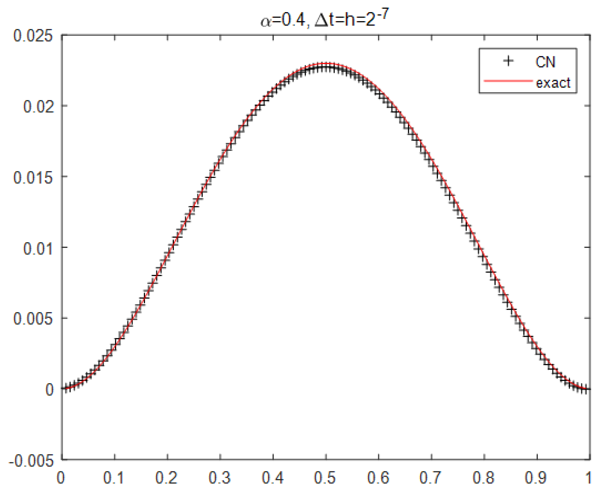
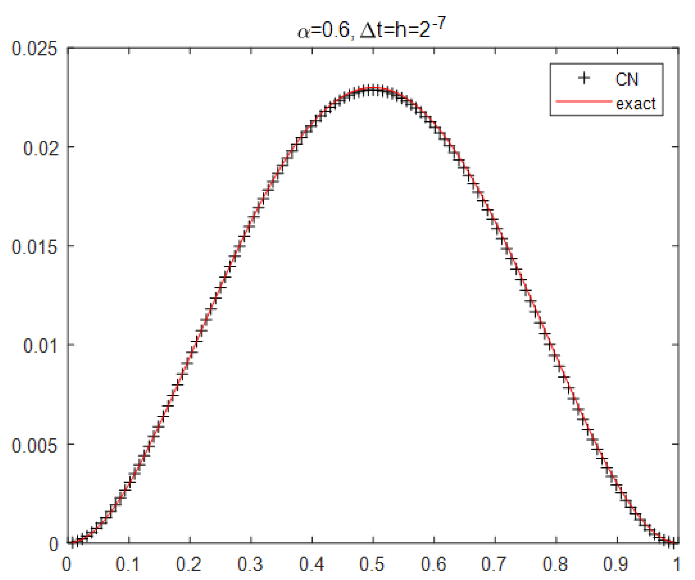
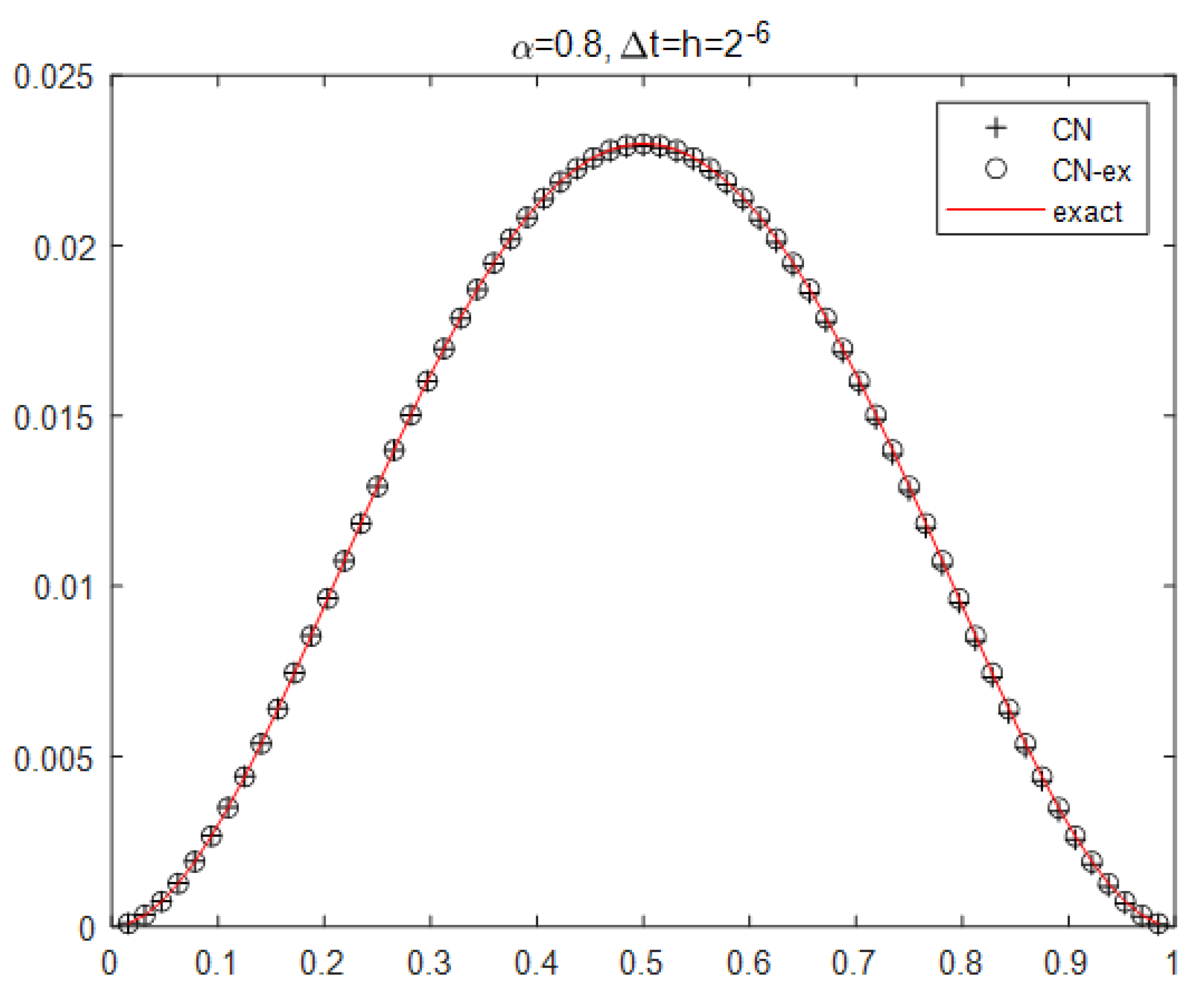
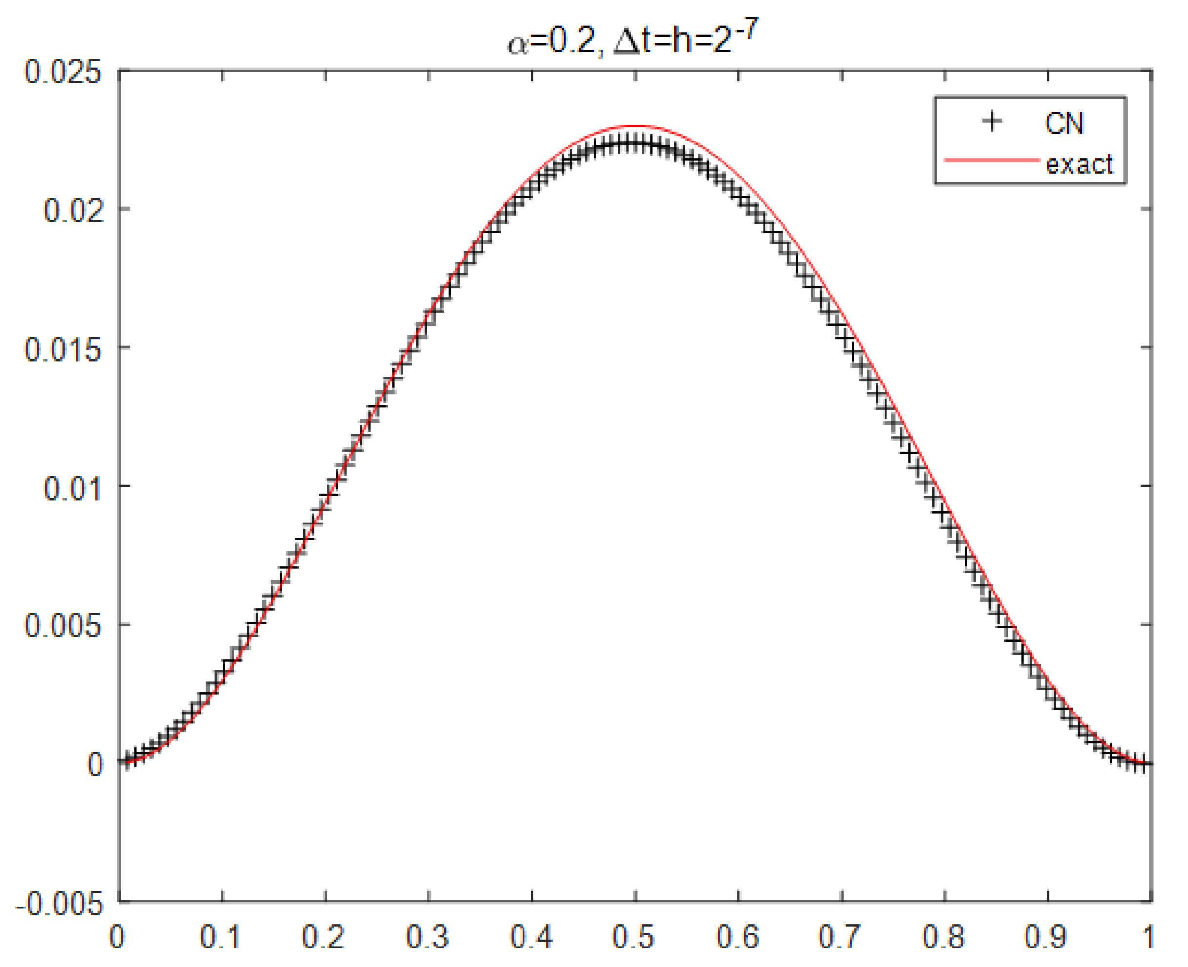
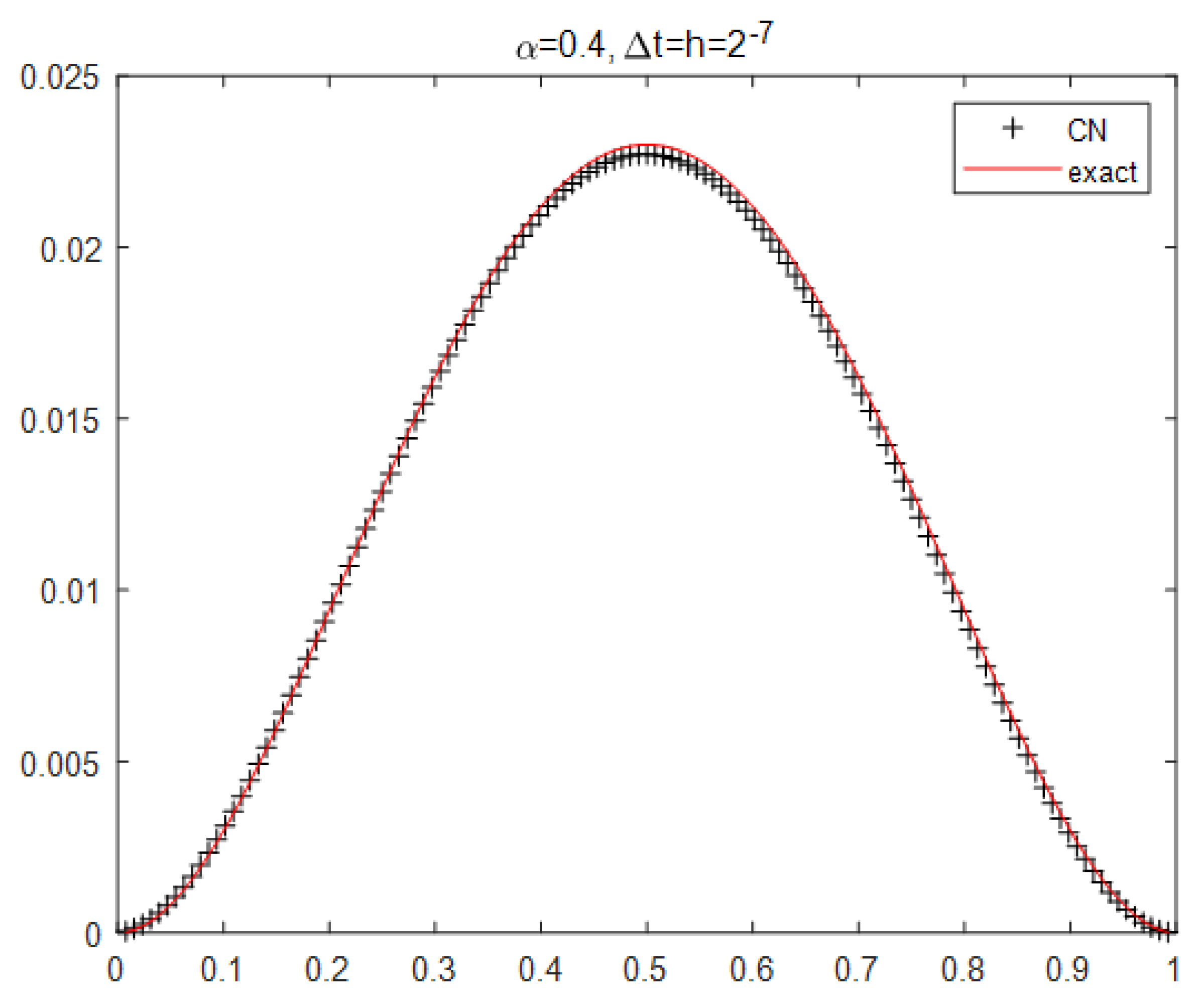
4. Numerical Example

In this section, we carry out two numerical experiments to demonstrate the effectiveness of the second-order accurate finite difference method. $\parallel e_h^N{\parallel }_{\infty }$ the maximum error of the Crank-Nicolson numerical solution, $\parallel e_h^{N-ex}{\parallel }_{\infty }$ the maximum error of the corresponding extrapolated Crank-Nicolson numerical solution.

Example 1 

(Parabolic case [22]). The following two-sided space-fractional diffusion equation was considered

$$\begin{gathered} \frac{\partial p(x,t)}{\partial t}=\frac{\partial }{\partial x}(C\left(x\right)\frac{{\partial }^{\alpha }p(x,t)}{\partial x^{\alpha }}-D\left(x\right)\frac{{\partial }^{\alpha }p(x,t)}{\partial {(-x)}^{\alpha }})+f(x,t), \\ a\le x\le b,0<\alpha <1,0\le t\le T. \end{gathered}$$

(24)

The finite domain is $[0,1]$. The nonnegative diffusion coefficient $C\left(x\right)=\frac{1-x^2}{2}$, $D\left(x\right)=\frac{1+x^2}{2}$. The source term $f(x,t)$ is given by

$$f(x,t)=-e^{-t}[x^2{(1-x)}^2-xq(x,\alpha )+\frac{1-x^2}{2}q(x,1+\alpha )-xq(1-x,\alpha )+\frac{1+x^2}{2}q(1-x,1+\alpha )],$$

(25)

here

$$q(x,t)=\frac{\mathsf{\Gamma }\left(5\right)}{\mathsf{\Gamma }(5-\alpha )}{x}^{4-\alpha }-\frac{2\mathsf{\Gamma }\left(4\right)}{\mathsf{\Gamma }(4-\alpha )}{x}^{3-\alpha }+\frac{\mathsf{\Gamma }\left(3\right)}{\mathsf{\Gamma }(3-\alpha )}{x}^{2-\alpha }.$$

(26)

The exact solution to this problem is

$$p(x,t)=e^{-t}{x}^2{(1-x)}^2,$$

(27)

which satisfies the initial function

$$\varphi \left(x\right)=x^2{(1-x)}^2,$$

(28)

and the Dirichlet boundary conditions are

$$p(0,t)=p(1,t)=0.$$

(29)

In the numerical experiments, we consider four different α in the case, respectively.

Table 1. Error behaviors and rate with $\alpha =0.2,0.4,0.6$ at time $T=1$ for Example 1.

	$\alpha =0.2$		$\alpha =0.4$		$\alpha =0.6$
$\mathbf{\Delta }\mathit{t}\mathbf{=}\mathit{h}$	$\parallel e_h^N{\parallel }_{\infty }$	$\mathit{Rate}$	$\parallel e_h^N{\parallel }_{\infty }$	$\mathit{Rate}$	$\parallel e_h^N{\parallel }_{\infty }$	$\mathit{Rate}$
$2^{-3}$	7.5340 $\times {10}^{-3}$	-	4.2000 $\times {10}^{-3}$	-	1.9000 $\times {10}^{-3}$	-
$2^{-4}$	4.2214 $\times {10}^{-3}$	1.78	2.4000 $\times {10}^{-3}$	1.75	1.2000 $\times {10}^{-3}$	1.83
$2^{-5}$	2.2199 $\times {10}^{-3}$	1.90	1.3000 $\times {10}^{-3}$	1.85	6.565 $\times {10}^{-4}$	1.58
$2^{-6}$	1.1356 $\times {10}^{-3}$	1.95	6.4325 $\times {10}^{-4}$	2.02	3.4039 $\times {10}^{-4}$	1.93
$2^{-7}$	5.7351 $\times {10}^{-4}$	1.98	3.2425 $\times {10}^{-4}$	1.98	1.7301 $\times {10}^{-4}$	1.97

shows the convergence rates of the numerical solutions of Example 1 with $\alpha =0.2,0.4,0.6$ at the time $T=1$. The numerical solution matches the exact analytical solution of the fractional differential equation. It shows stability and a convergence order of $O({(\Delta t)}^2+h)$. Figure 1 shows the numerical solution in Crank-Nicolson format and the exact solution of Example 1, where $\alpha =0.2$, $\Delta t=h=2^{-7}$ at time $T=1$. Figure 2 shows the numerical solution in Crank-Nicolson format and the exact solution of Example 1, where $\alpha =0.4$, $\Delta t=h=2^{-7}$ at time $T=1$. Figure 3 shows the numerical solution in Crank-Nicolson format and the exact solution of Example 1, where $\alpha =0.6$, $\Delta t=h=2^{-7}$ at time $T=1$. The numerical solution compares well with the exact analytic solution to the fractional partial differential equation in this test case.

To check the speed of convergence of this method, we start with $\Delta t=h=2^{-3}$. To obtain an extrapolated CN solution on this grid size, in the first step the problem is solved numerically $p_{x,h}^{t_n}$ on a coarse grid with $\Delta t=h=2^{-3}$ and in the second step a finer grid size is created using the same and in the second step a finer grid size is created using the same $\Delta t$ but halving h ($\Delta t=2^{-3}$,$h=2^{-4}$). The third step is to calculate the extrapolation solution for the points on the coarse grid as $p_x^{t_n}=2p_{x,h/2}^{t_n}-p_{x,h}^{t_n}$.

For Example 1 with $T=1$ and $\alpha =0.8$,

Table 2. Error behaviors and rate for the Crank-Nicolson scheme and exact solution for Example 1 with $\alpha =0.8$ at time $T=1$.

$\mathbf{\Delta }\mathit{t}\mathbf{=}\mathit{h}$	$\parallel {\mathit{e}}_{\mathit{h}}^{\mathit{N}}{\parallel }_{\mathit{\infty }}$	$\mathit{Rate}$	$\mathbf{\parallel }{\mathit{e}}_{\mathit{h}}^{\mathit{N}\mathbf{-}\mathit{ex}}{\mathbf{\parallel }}_{\mathit{\infty }}$	$\mathit{Rate}$
$2^{-3}$	7.7198 $\times {10}^{-4}$	-	7.4596 $\times {10}^{-4}$	-
$2^{-4}$	4.0338 $\times {10}^{-4}$	1.91	1.7406 $\times {10}^{-4}$	4.29
$2^{-5}$	2.4992 $\times {10}^{-4}$	1.61	4.1151 $\times {10}^{-5}$	4.23
$2^{-6}$	1.3734 $\times {10}^{-4}$	1.82	9.7767 $\times {10}^{-6}$	4.21

shows the absolute error in the numerical solution. The second column shows the absolute value of the maximum error in the numerical solution. The third column shows the rate of reduction of the error as the mesh is refined. It shows the order of convergence as $O({(\Delta t)}^2+h)$. The fourth column shows the maximum absolute error for the Crank-Nicholson extrapolation. The last column shows the error rate of these extrapolated solutions. We note that the order of convergence is second order $O({(\Delta t)}^2+h^2)$. Figure 4 shows the numerical solution for the Crank-Nicolson scheme and the extrapolated Crank-Nicolson scheme and rate for Example 1 with $\alpha =0.8$, $\Delta t=h=2^{-6}$ at time $T=1$.

Example 2 

(Linear case [22]). The following two-sided space-fractional diffusion equation was considered

$$\begin{gathered} \frac{\partial p(x,t)}{\partial t}=\frac{\partial }{\partial x}(C\left(x\right)\frac{{\partial }^{\alpha }p(x,t)}{\partial x^{\alpha }}-D\left(x\right)\frac{{\partial }^{\alpha }p(x,t)}{\partial {(-x)}^{\alpha }})+f(x,t), \\ a\le x\le b,0<\alpha <1,0\le t\le T. \end{gathered}$$

(30)

The finite domain is $[0,1]$. The nonnegative diffusion coefficient $C\left(x\right)=2-x$, $D\left(x\right)=2+x$. The source term $f(x,t)$ is given by

$$f(x,t)=-e^{-t}[x^2{(1-x)}^2-q(x,\alpha )+(2-x)q(x,1+\alpha )-q(1-x,\alpha )+(2+x)q(1-x,1+\alpha )],$$

(31)

here

$$q(x,t)=\frac{\mathsf{\Gamma }\left(5\right)}{\mathsf{\Gamma }(5-\alpha )}{x}^{4-\alpha }-\frac{2\mathsf{\Gamma }\left(4\right)}{\mathsf{\Gamma }(4-\alpha )}{x}^{3-\alpha }+\frac{\mathsf{\Gamma }\left(3\right)}{\mathsf{\Gamma }(3-\alpha )}{x}^{2-\alpha }.$$

(32)

The exact solution to this problem is

$$p(x,t)=e^{-t}{x}^2{(1-x)}^2,$$

(33)

which satisfies the initial function

$$\varphi \left(x\right)=x^2{(1-x)}^2,$$

(34)

and the Dirichlet boundary conditions are

$$p(0,t)=p(1,t)=0.$$

(35)

In the numerical experiments, we consider four different α values in the case, respectively.

Table 3. Error behaviors and rate with $\alpha =0.2,0.4,0.6$ at time $T=1$ for Example 2.

	$\mathit{\alpha }=0.2$		$\mathit{\alpha }=0.4$		$\mathit{\alpha }=0.6$
$\mathbf{\Delta }\mathit{t}\mathbf{=}\mathit{h}$	$\mathbf{\parallel }{\mathit{e}}_{\mathit{h}}^{\mathit{N}}{\mathbf{\parallel }}_{\mathit{\infty }}$	$\mathit{Rate}$	$\mathbf{\parallel }{\mathit{e}}_{\mathit{h}}^{\mathit{N}}{\mathbf{\parallel }}_{\mathit{\infty }}$	$\mathit{Rate}$	$\mathbf{\parallel }{\mathit{e}}_{\mathit{h}}^{\mathit{N}}{\mathbf{\parallel }}_{\mathit{\infty }}$	$\mathit{Rate}$
$2^{-3}$	8.3000 $\times {10}^{-3}$	-	3.8000 $\times {10}^{-3}$	-	1.3000 $\times {10}^{-3}$	-
$2^{-4}$	5.0000 $\times {10}^{-3}$	1.66	2.3000 $\times {10}^{-3}$	1.75	9.1101 $\times {10}^{-4}$	1.43
$2^{-5}$	2.7000 $\times {10}^{-3}$	1.85	1.2000 $\times {10}^{-3}$	1.85	5.1674 $\times {10}^{-4}$	1.76
$2^{-6}$	1.4000 $\times {10}^{-3}$	1.93	6.4069 $\times {10}^{-4}$	2.02	2.7250 $\times {10}^{-4}$	1.90
$2^{-7}$	7.1602 $\times {10}^{-4}$	1.96	3.2564 $\times {10}^{-4}$	1.98	1.3953 $\times {10}^{-4}$	1.95

shows the convergence rates for the numerical solutions of Example 2 with $\alpha =0.2,0.4,0.6$ at the time $T=1$. In this test case the numerical solution agrees well with the exact analytical solution of the fractional order partial differential equation. It shows stability and a convergence order of $O({(\Delta t)}^2+h)$. Figure 5 shows the numerical solution in Crank-Nicolson format and the exact solution of Example 2 with $\alpha =0.2$, $\Delta t=h=2^{-7}$ at time $T=1$. Figure 6 shows the numerical solution in Crank-Nicolson format and the exact solution of Example 4.2 with $\alpha =0.4$, $\Delta t=h=2^{-7}$ at time $T=1$. Figure 7 shows the numerical solution in Crank-Nicolson format and the exact solution of Example 2 with $\alpha =0.6$, $\Delta t=h=2^{-7}$ at time $T=1$. The numerical solution compares well with the exact analytic solution to the fractional partial differential equation in this test case.

Table 4. Error behaviors and rate for the Crank-Nicolson scheme and exact solution for Example 2 with $\alpha =0.8$ at time $T=1$.

$\mathbf{\Delta }\mathit{t}\mathbf{=}\mathit{h}$	$\mathbf{\parallel }{\mathit{e}}_{\mathit{h}}^{\mathit{N}}{\mathbf{\parallel }}_{\mathit{\infty }}$	$\mathit{Rate}$	$\parallel {\mathit{e}}_{\mathit{h}}^{\mathit{N}-\mathit{ex}}{\parallel }_{\mathit{\infty }}$	$\mathit{Rate}$
$2^{-3}$	7.1922 $\times {10}^{-4}$	-	6.5386 $\times {10}^{-4}$	-
$2^{-4}$	1.8018 $\times {10}^{-4}$	3.99	1.5769 $\times {10}^{-4}$	4.15
$2^{-5}$	1.3921 $\times {10}^{-4}$	1.29	3.7662 $\times {10}^{-5}$	4.19
$2^{-6}$	8.2345 $\times {10}^{-5}$	1.69	8.2345 $\times {10}^{-5}$	4.57

shows the absolute error in the numerical solution for Example 2 at time $T=1$ and $\alpha =0.8$. The second column shows the absolute value of the maximum error in the numerical solution. The third column shows the rate of reduction of the error as the mesh is refined. It shows the order of convergence as $O({(\Delta t)}^2+h)$. The fourth column shows the maximum absolute error for the Crank-Nicholson extrapolation. The last column shows the error rate of these extrapolated solutions. We note that the order of convergence is second order $O({(\Delta t)}^2+h^2)$. Figure 8 shows the numerical solution for the Crank-Nicolson scheme and the extrapolated Crank-Nicolson scheme and rate for Example 2 with $\alpha =0.8$, $\Delta t=h=2^{-6}$ at time $T=1$.

5. Conclusions

In this paper, we have considered a two-sided spatial fractional order diffusion equation with variable diffusion coefficients from a fractional Fick’s law. Although finite difference estimates for the fractional order derivatives have been elusive, a high precision convergence method for the superdiffusion equation is feasible by applying the extrapolation to the Crank-Nicolson method and the Richardson method, in combination with the Grünwald estimates using shifts. We can obtain second-order accurate numerical estimates in time and space using the CN and Richardson extrapolation methods. We then consider more general cases, such as the case where $C\left(x\right)$ and $D\left(x\right)$ are not monotonic, or higher accuracy differential methods. We also look at numerical solutions of this equation for different boundary conditions, such as fractional boundary conditions.

References

1. Sokolov, L.M.; Klafer, J.; Blumen, A. Fractional kinetics. Phys. Today 2002, 55, 48–54. [Google Scholar] [CrossRef]
2. Magin, R.L. Fractional Calculus in Bioengineering, Bioengineering; Begell House Publishers: Danbury, CT, USA, 2006. [Google Scholar]
3. Kirchner, J.W.; Feng, X.; Neal, C. Fractal stream chemistry and its implications for contaminant transport in catchments. Nature 2000, 403, 524–527. [Google Scholar] [CrossRef]
4. Raberto, M.; Scalas, E.; Mainardi, F. Waiting-times and returns in high-frequency financial data: An empirical study. Phys. Stat. Mech. Its Appl. 2002, 314, 749–755. [Google Scholar] [CrossRef] [Green Version]
5. Liu, F.; Zhuang, P.; Turner, I.; Anh, V.; Burrage, K. A semi-alternating direction method for a 2-D fractional FitzHugh-Nagumo monodomain model on an approximate irregular domain. J. Comput. Phys. 2015, 293, 252–263. [Google Scholar] [CrossRef] [Green Version]
6. Li, S.; Cao, W.; Wang, Y. On spectral Petrov-Galerkin method for solving optimal control problem governed by a two-sided fractional diffusion equation. Comput. Math. Appl. 2022, 107, 104–116. [Google Scholar] [CrossRef]
7. She, Z.H.; Qu, H.D.; Liu, X. Stability and convergence of finite difference method for two-sided space-fractional diffusion equations. Comput. Math. Appl. 2021, 89, 78–86. [Google Scholar] [CrossRef]
8. Hao, Z.P.; Lin, G.; Zhang, Z.Q. Error estimates of a spectral Petrov-Galerkin method for two-sided fractional reaction-diffusion equations. Appl. Math. Comput. 2020, 374, 125045. [Google Scholar] [CrossRef]
9. Li, S.; Zhou, Z. Fractional spectral collocation method for optimal control problem governed by space fractional diffusion equation. Appl. Math. Comput. 2019, 350, 331–347. [Google Scholar] [CrossRef]
10. Gunzburger, M.; Wang, J. Error analysis of fully discrete finite element approximations to an optimal control problem governed by a time-fractional PDE. SIAM J. Control. Optim. 2019, 57, 241–263. [Google Scholar] [CrossRef]
11. Ozbilge, E.; Kanca, F.; Zbilge, E. Inverse Problem for a Time Fractional Parabolic Equation with Nonlocal Boundary Conditions. Mathematics 2022, 10, 1479. [Google Scholar] [CrossRef]
12. Feng, L.B.; Zhuang, P.; Liu, F.; Turner, I. Stability and convergence of a new finite volume method for a two-sided space-fractional diffusion equation. Appl. Math. Comput. 2015, 257, 52–65. [Google Scholar] [CrossRef] [Green Version]
13. Liu, X.Y.; Liu, Z.H.; Fu, X. Relaxation in nonconvex optimal control problems described by fractional differential equations. J. Math. Anal. Appl. 2014, 409, 446–458. [Google Scholar] [CrossRef]
14. Jia, J.; Wang, H. Fast finite difference methods for space-fractional diffusion equations with fractional derivative boundary conditions. J. Comput. Phys. 2015, 293, 359–369. [Google Scholar] [CrossRef]
15. Lai, J.J.; Liu, H.Y. On a Novel Numerical Scheme for Riesz Fractional Partial Differential Equations. Mathematics 2021, 9, 1–14. [Google Scholar] [CrossRef]
16. Chen, H.B.; Gan, S.Q.; Xu, D.; Liu, Q.W. A second-order BDF compact difference scheme for fractional-order Volterra equation. Int. J. Comput. Math. 2016, 93, 1140–1154. [Google Scholar] [CrossRef]
17. Ma, C.Y.; Shiri, B.; Wu, G.C.; Baleanu, D. New fractional signal smoothing equations with short memory and variable order. Optik 2020, 218, 164507. [Google Scholar] [CrossRef]
18. Shiri, B.; Kong, H.; Wu, G.C. Adaptive Learning Neural Network Method for Solving Time-Fractional Diffusion Equations. Neural Comput. 2022, 34, 971–990. [Google Scholar] [CrossRef]
19. Qu, W.; Lei, S.L.; Vong, S.W. A note on the stability of a second order finite difference scheme for space fractional diffusion equations, Numerical Algebra. Control. Optim. 2014, 4, 317–325. [Google Scholar]
20. Sitho, S.; Ntouyas, S.K.; Sudprasert, C.; Tariboon, J. Integro-Differential Boundary Conditions to the Sequential -Hilfer and -Caputo Fractional Differential Equations. Mathematics 2023, 11, 867. [Google Scholar] [CrossRef]
21. Hakkar, N.; Dhayal, R.; Debbouche, A.; Torres, D.F.M. Approximate Controllability of Delayed Fractional Stochastic Differential Systems with Mixed Noise and Impulsive Effects. Fractal Fract. 2023, 7, 104. [Google Scholar] [CrossRef]
22. Chen, S.; Liu, F.; Jiang, X.; Turner, I.; Anh, V. A fast semi-implicit difference method for a nonlinear two-sided space-fractional diffusion equation with variable diffusivity coefficient. Appl. Math. Comput. 2015, 257, 591–601. [Google Scholar] [CrossRef] [Green Version]
23. Podlubny, I. Fractional Differential Equations; Academic Press: New York, NY, USA, 1999. [Google Scholar]
24. Meerschaert, M.M.; Sikorskii, A. Stochastic Models for Fractional Calculus; De Gruyter: Berlin, Germany, 2012. [Google Scholar]
25. Tadjeran, C.; Meerschaert, M.M. Finite difference approximations for two-sided space-fractional partial differential equations. Appl. Numer. Math. 2006, 56, 80–90. [Google Scholar]
26. Samko, S.G.; Kilbas, A.A.; Marichev, O.I. Fractional Integrals and Derivatives, Theory and Applications; Gordon Breach: London, UK, 1993. [Google Scholar]
27. Isaacson, E.; Keller, H.B.; Weiss, G.H. Analysis of Numerical Methods; Wiley: New York, NY, USA, 1966. [Google Scholar]
28. Tadjeran, C.; Meerschaert, M.M.; Scheffler, P. A second-order accurate numerical approximation for the fractional diffusion equation. J. Comput. Phys. 2006, 213, 205–213. [Google Scholar] [CrossRef]
29. Richtmyer, R.D.; Morton, K.W. Difference Methods for Initial-Value Problems; Krieger Publishing: Malabar, FL, USA, 1994. [Google Scholar]
Figure 1. The numerical solution for the Crank-Nicolson scheme and exact solution for Example 1 with α = 0.2 , Δ t = h = 2 7 at time T = 1 .
Mathematics 11 01838 g001
Figure 2. The numerical solution for the Crank-Nicolson scheme and exact solution for Example 1 with α = 0.4 , Δ t = h = 2 7 at time T = 1 .
Mathematics 11 01838 g002
Figure 3. The numerical solution for the Crank-Nicolson scheme and exact solution for Example 1 with α = 0.6 , Δ t = h = 2 7 at time T = 1 .
Mathematics 11 01838 g003
Figure 4. The numerical solution for the Crank-Nicolson scheme and the extrapolated Crank-Nicolson scheme and rate for Example 1 with α = 0.8 , Δ t = h = 2 6 at time T = 1 .
Mathematics 11 01838 g004
Figure 5. The numerical solution for the Crank-Nicolson scheme and exact solution for Example 2 with α = 0.2 , Δ t = h = 2 7 at time T = 1 .
Mathematics 11 01838 g005
Figure 6. The numerical solution for the Crank-Nicolson scheme and exact solution for Example 2 with α = 0.4 , Δ t = h = 2 7 at time T = 1 .
Mathematics 11 01838 g006
Figure 7. The numerical solution for the Crank-Nicolson scheme and exact solution for Example 2 with α = 0.6 , Δ t = h = 2 7 at time T = 1 .
Mathematics 11 01838 g007
Figure 8. The numerical solution for the Crank-Nicolson scheme and the extrapolated Crank-Nicolson scheme and exact solution for Example 2 with α = 0.8 , Δ t = h = 2 6 at time T = 1 .
Mathematics 11 01838 g008