Article

Reconstructing the Quarterly Series of the Chilean Gross Domestic Product Using a State Space Approach

by
Christian Caamaño-Carrillo
1,*,†,
Sergio Contreras-Espinoza
1,† and
Orietta Nicolis
2,†
1
Departament of Statistics, Faculty of Science, Universidad del Bío-Bío, Concepción 4081112, Chile
2
Faculty of Engineering, Universidad Andres Bello, Viña del Mar 2520000, Chile
*
Author to whom correspondence should be addressed.
These authors contributed equally to this work.
Mathematics 2023, 11(8), 1827; https://doi.org/10.3390/math11081827
Submission received: 20 December 2022 / Revised: 17 February 2023 / Accepted: 8 March 2023 / Published: 12 April 2023
(This article belongs to the Special Issue Probability, Statistics & Symmetry)

Abstract

:
In this work, we use a cointegration state space approach to estimate the quarterly series of the Chilean Gross Domestic Product (GDP) in the period 1965–2009. First, the equation of Engle–Granger is estimated using the data of the yearly GPD and some related variables, such as the price of copper, the exports of goods and services, and the mining production index. The estimated coefficients of this regression are then used to obtain a first estimation of the quarterly GDP series with measurement errors. A state space model is then applied to improve the preliminary estimation of the GDP with the main purpose of eliminating the maximum error of measurement such that the sum of the three-month values coincide swith the yearly GDP. The results are then compared with the traditional disaggregation methods. The resulting quarterly GDP series reflects the major events of the historical Chilean economy.

1. Introduction

An important limitation in describing the Chilean economy is the unavailability of a sufficient number of observations for estimating a reliable econometric model. Among the economic variables, the gross domestic product (GDP) is one of the most important indexes for describing the country’s economy. It constitutes the broadest measure of the country’s economy, containing a wide range of constitutive factors representing different areas of economic activity. It can be defined as the total value of products and services produced by a nation in a specific period of time, usually a year or a quarter. The frequency with which GDP is calculated is of particular interest since the low number of data (for example, yearly) could cause serious problems in terms of the quality of quantitative analysis. However, for this variable, in Chile, there is no quarterly information before 1986 (only annual information is available), and there is not a formally recognized procedure for reconstructing it. The Benchmarking or disaggregation methods allow disaggregating or interpolating a low frequency to a higher frequency time series, while the sum remains consistent with the low-frequency series. The most used disaggregation methods in the literature for estimating the GDP of different countries have been proposed by [1,2,3,4,5,6]. In summary, a two-step procedure can be used to describe all these methods. First, a preliminary high-frequency series is evaluated by using indicators with the same frequency. Second, the differences between the preliminary low-frequency series and the observed series are distributed among the high-frequency series. The resulting estimated high-frequency series is obtained by the sum of the preliminary high-frequency series and distributed annual residuals. While the methods of Denton [4] and Denton–Cholette [3] attempt to preserve the movements by using a single indicator as their preliminary series (which is not necessarily correlated with the low-frequency series), Chow–Lin [2], Fernandez [5], and Litterman [6] performed a Generalized Least Squares Regression (GLS) of the low-frequency series on the high-frequency one for evaluating the preliminary series, which is obtained by the fitted values of the GLS regression. In the second step, the distribution matrix of all temporal disaggregation methods (except for the Denton–Cholette method) is a function of the variance-covariance matrix, as shown in Table 2 of [7]. While Denton proposed to minimize the squared absolute or relative deviations from a (differenced) indicator series, Denton–Cholette introduced a modification of Denton’s original method, which removes spurious transient movement at the beginning of the resulting series ([7,8]). Instead, Chow–Lin [2] assumed that the high-frequency residuals follow a stationary autoregressive process of order 1, AR(1), while Fernandez [5] and Litterman [6] suppose that the quarterly residuals follow a nonstationary process where the residual term is an AR(1). In particular, Fernandez’s method is a special case of Litterman where the autoregression parameter is equal to zero, and the high-frequency residuals follow a random walk process. Several methods have been proposed for estimating the autoregressive parameter (denoted by ρ ) of the residuals in the Chow–Lin and Litterman methods. Chow and Lin (1971) proposed an iterative procedure that infers the parameter from the observed autocorrelation of the low-frequency residuals. Bournay and Laroque [9] suggested the maximization of the likelihood of the GLS regression, and Barbone et al. [10] proposed the minimization of the weighted residual sum of squares (RSS). Two variants of minimization of the residual sum of squares of the Chow–Lin method have been proposed: one of these was originally implemented in the software Ecotrim introduced by Barcellan et al. [1], which used the correlation matrix instead of the variance-covariance matrix, and the other one in Matlab, by Quilis [11], which multiplied the correlation matrix by a factor of 1 / ( 1 ρ 2 ) . All the above methods are now implemented in the tempdisagg R package [7]. Further, some works compare the above-mentioned methods using some traditional accuracy prediction metrics, such as Root Mean Squared Error (RMSE), Absolute Mean Difference (MAD), and Theil’s inequality coefficient (see, for example, [12,13,14]). In particular, Ajao et al. [14] compared the results of disaggregating techniques (Denton, Denton–Cholette, Chow–Lin, and Fernandez, and Litterman) for studying the Annual Gross Domestic Product (GDP) for Nigeria in the period 1981–2012 using quarterly export and import as the indicator variables. Some of these methods are also compared by Islaqm [12] for disaggregating the yearly export of Bangladesh to quarterly export in the period 2004–2012. In [13], different methods were used to disaggregate the annual series for personal consumption using the quarterly disposable income as an indicator.
Extensions to a dynamic framework have been considered by Guay and Maurin [15,16,17]. In particular, [16] extended the Chow–Lin procedure to flexible dynamic setting taking into account seasonality or calendar effects. Reference [15] presented a temporal disaggregation technique concerning the extension from static to dynamic autoregressive distributed lag regressions in a state-space framework with application to the Italian quarterly accounts. In [17], a state space approach is proposed for the temporal disaggregation problem by considering dynamic regression models with a particular concentration on the exact initialization of the different models. A set of annual series and the corresponding quarterly indicators, available by the Italian National Statistical Institute, Istat, are considered for real case studies. A different approach based on a two-step procedure (cointegration and state space regression) has been proposed by [18] for estimating the Brazilian GDP quarterly series in the period between 1960 and 1996. A different type of two-step procedure based on regression and Benchmarking has been proposed by [19] for the temporal disaggregation of quarterly GDP, and a novel sparse temporal-disaggregation procedure with an application to the UK gross domestic product data has been introduced by [20].
GPD is important because it represents an image of how a country’s finances are doing and which areas are growing or shrinking. The growth of the PIB, which compares one quarter or one year with another, provides a reference to know if the economic situation is improving or worsening. PIB may be affected by many factors, such as public spending, trade, foreign investment, and productivity, and is a good financial indicator. When the PIB of a country grows, it means that its economy is prosperous. Companies are more profitable, they hire more people, and the investors will want to invest in the companies of the country. On the contrary, when the gross domestic product of a nation decreases, it means that its economy is experiencing a slowdown. The economic slowdown translates into less hiring of personnel, thus increases the unemployment rate. In addition, the profits of many companies decrease, so the distribution of dividends and the prices of their shares can also fall. The availability of official information produced by the state covers from 1940 to the present. The systematic construction of national accounts begins in CORFO (1957), which represents series prior to 1940–1954. This is followed by the accounts prepared by the Planning Office (ODEPLAN), which basically cover the decade of the nineteen-sixties. Finally, to this day, it is the Central Bank of Chile that is in charge of this task. The Central Bank of Chile has calculated the national accounts using 1977, 1986, 1996, and 2003 as base years. [21]).
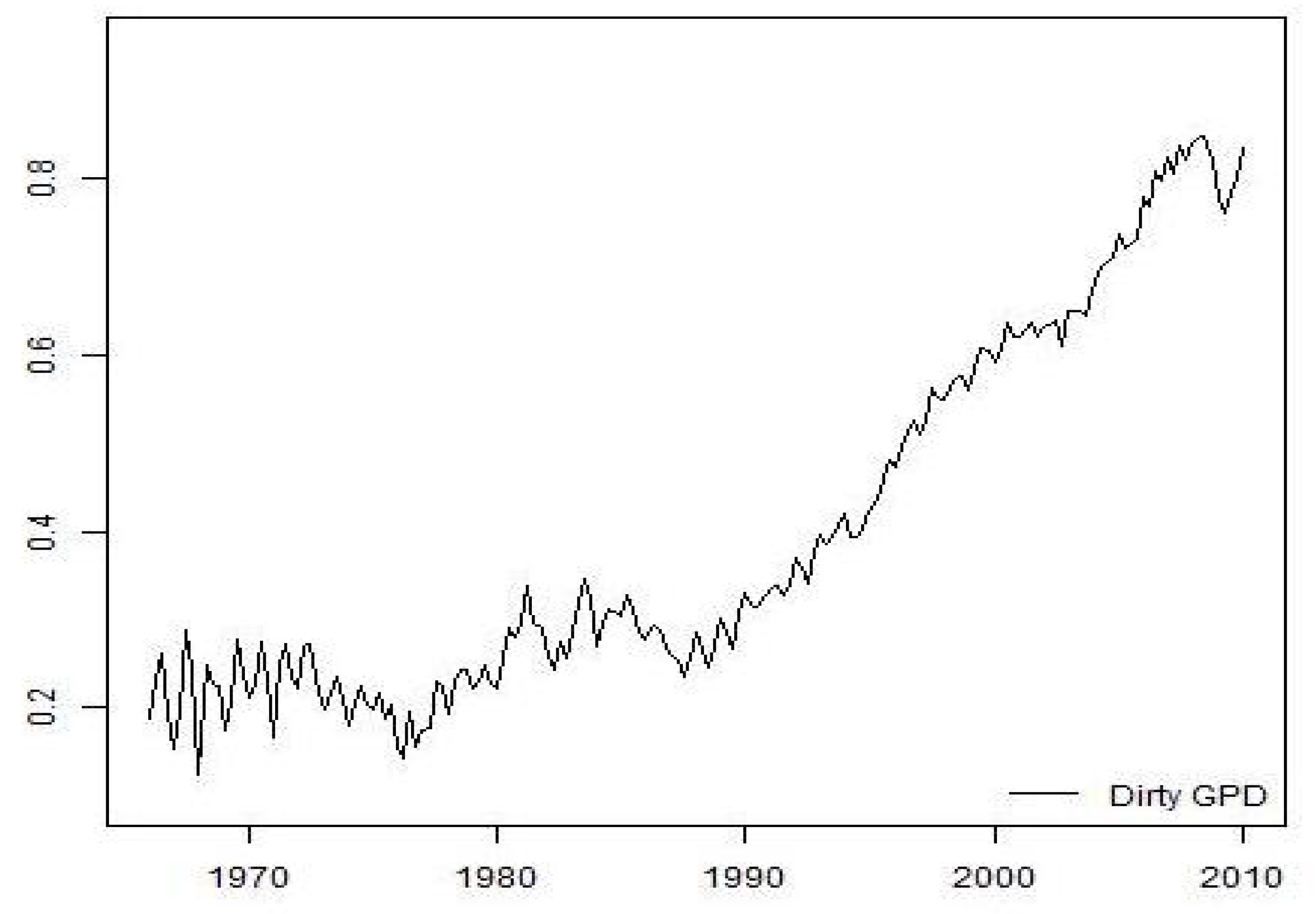
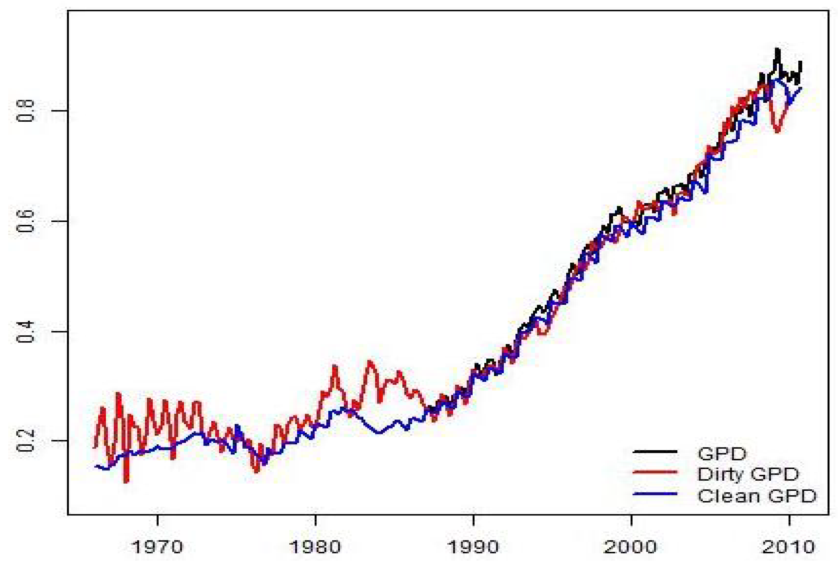
The main objective of this work is to propose a methodology for the estimation of Chilean quarterly GDP from 1965 to 2009. The procedure consists of an initial estimate of the quarterly GDP, which is obtained through the static Engle–Granger equation (see [22,
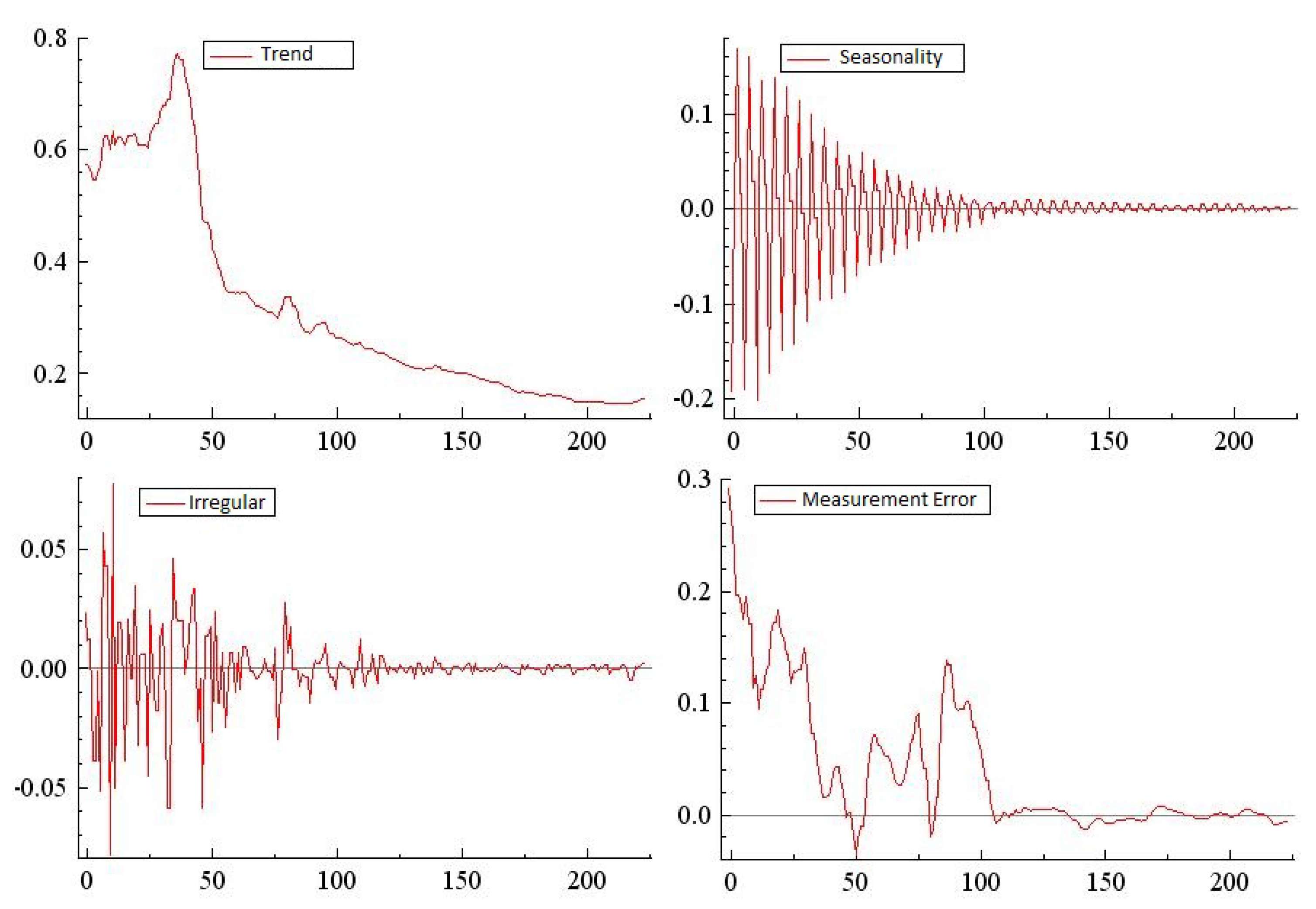
23]) or cointegration analysis using the annual GDP data and variables related to GDP. The estimated coefficients of this regression are used to construct a quarterly equation between GDP and related variables by interpolating the estimated coefficients with the quarterly data of the aforementioned variables. This equation produces a first estimate of the quarterly GDP, called dirty GDP, due to the presence of errors. The second stage is to improve the estimates by minimizing the measurement errors and considering that the estimated measurements should be consistent with the annual GDP calculated by the Central Bank of Chile; that is, the sum of the quarterly estimates should be equal to the total annual GDP. The process of harmonization of quarterly and annual estimates is known, in the literature, as Benchmarking, and in this paper, it is addressed using the state space approach (see [24,25]). Important economical Chilean variables, such as the monetary aggregate, the price of copper, the terms of trade, the exports of goods and services and the mining production index, are used in the model to improve the estimation of the quarterly data. The application of the proposed method for reconstructing the quarterly Chilean GDP series constitutes a new contribution, which could be helpful to better understand the history of the Chilean economy additionally to the possibility of applying econometric models for predicting its future behavior. In summary, the main contributions of this work can be described as follows.
  • Our proposal allows the introduction of a new method that is comparable with other methods used in other countries. Nowadays, there is no official method in Chile for reconstructing high-frequency series from low-frequency data.
  • The proposed method allows the reconstruction of the GDP series in a critical historical period of Chile and better interpretation of the behavior of the economy of this country. In the new version of the paper, we have included a historical note of the period under study.
  • Different from the traditional methods that are used for forward interpolation, the proposed method allows the reconstruction of high-frequency time series backward, which is very important for interpreting the economical situation of Chile. Further, this method could be applied to interprete economic variables of other countries in the world.
  • From the methodological point of view, the state space approach for Benchmarking allows the elimination of measurement errors and assumptions such that the sum of the three-month values coincides with the yearly GDP.
The article is organized as follows: Section 2 briefly analyzes the methods used for the estimation of the quarterly GDP; Section 3 shows the results obtained by the estimated models. Finally, a discussion and conclusions are presented in Section 4 and Section 5, respectively.

2. Materials and Methods

2.1. Engle–Granger Cointegration Analysis

Cointegration analysis is a frequently used technique in the study of time series. The concept of cointegration was introduced by Granger and subsequently studied in depth in [22,23]. This technique emerges as a procedure that allows the discrimination between real relationships and spurious relationships between variables. A spurious regression arises when we try to relate two variables when there is no type of cause-effect relationship through regression, and it is erroneously concluded, after regression, that such a relationship exists. According to what is stated in [26], one of the characteristics of spurious relations consists of having a very high coefficient of determination and a Durbin–Watson statistic close to zero.
From an econometric point of view, two or more time series with integration order I ( 1 ) are cointegrated if there exists a linear combination of those series that has a lower order of integration, that is, I ( 0 ) . From an economic point of view, cointegration can be seen as a long-term equilibrium relationship between variables, such that these variables can deviate from the equilibrium situation in the short term, but with time, they will return to equilibrium. Another definition from the economic point of view says that two or more series are cointegrated if they move together over time and the differences between them are stable, i.e., stationary, even when each series is not stationary. The differences (or error term) in the cointegration equation are interpreted as the imbalance error for each particular point in time.

2.2. Benchmarking Method

According to [27], the concept of Benchmarking can be seen as a special form of signal extraction, which occurs when two (or more) data sources are available for the same target variable, which have different temporal frequencies, for example, monthly vs. annual, monthly vs. quarterly, annual vs. quarterly, etc. Generally, the two data sources do not correspond; for example, the quarterly sums of the measurements of a variable are not equal to the corresponding annual measure. Moreover, one of the data sources is more accurate than the other: the least frequent it is usually the more accurate since it is normally originated by censuses, which are hypothetically assumed free of sampling errors. The most reliable source is considered a Benchmark (comparative framework).
More specifically, Benchmarking is the process of trying to fit the most frequent series to the Benchmark. This is performed by decomposing the series into its structural elements: trend, seasonality, cycle, irregularities, and measurement errors, where the sum of these elements excludes the error.
According to [18], there are two main methods for applying Benchmarking to a time series: a purely numerical approach and a statistical method. The numerical approach covers the family of methods based on the minimization of a squared sum proposed by [4], and the statistical method, in turn, may be based on ARIMA processes such as those described by [28], the state space models proposed by [27], or the models that use a group of regressions, such as [29].

2.3. Methodological Procedure

2.3.1. First Stage: Analysis of Cointegration and Obtaining Dirty GDP

An initial estimate of the quarterly GDP is obtained through the static Engle–Granger equation or cointegration analysis using the data of annual GDP and variables related to GDP. Then, the estimated coefficients of the cointegrated model are used to interpolate the quarterly data, thus obtaining what is known as dirty GDP. The related variables to be used are: the monetary aggregate, the price of copper, the terms of trade, the exports of goods and services, and the mining production index. All these variables are available on the web page of the Central Bank of Chile (https://www.bcentral.cl (accessed on 14 October 2022)) on an annual and quarterly basis. Specifically, the calculation of dirty quarterly GDP is based on the estimation of a regression of GDP against the aforementioned series, with annual frequency expressed in base 1986 indices in order to obtain long-term coefficients that relate to the variables. After having estimated the cointegration vector by Ordinary Least Squares (OLS), we form a linear combination using the quarterly frequency series in order to obtain the interpolated series of the quarterly GDP. The estimated quarterly series are linked and compared to the series of the Central Bank of Chile, producing the dirty GDP series, which is refined in the second half of the procedure.
Prior to 1986, GDP data were only available on the annual frequency, which explains why the estimate was made on this frequency. It is of great importance that the estimated dirty GDP series incorporate the components present in the original series of GDP obtained by the Central Bank of Chile after 1986 and respect the annual information between 1965 and 2009 of the original series of GDP.
Therefore, dirty GDP is the first approximation of the quarterly GDP that recovers the lack of data prior to 1986 and that has a seasonal pattern thereafter that is identical to the series of the Central Bank of Chile.

2.3.2. Second Stage: State Space Models by Benchmarking and Obtaining Clean GDP

The state space approach provides a unified methodology for studying a wide variety of problems in time series. For example, by means of this approach, it is possible to model the behavior of the different components of a series separately and immediately combine these sub-models by obtaining a single model for the series of interest. In this context, the state space models are called Structural Models (see, for example, [24,25]). The state space models are formed by two types of variables: the non-observable variables of the state, which determine the movement of the system in time, and the observations of the series.
In general situations, the Gaussian general model of state space is defined by:
y t = Z t α t + ϵ t , ϵ t N ( 0 , H t ) , α t + 1 = T t α t + R t η t , η t N ( 0 , Q t ) , t = 1 , , n , w i t h α 1 N ( a 1 , P 1 )
where y t is a p × 1 vector of observations; α t is an unobserved vector of dimension m × 1 called state vector; and the terms of independent perturbations, ϵ t and η t are serially independent assumptions independent of each other at all times.
Matrices Z t , T t , R t , H t , and Q t , with the appropriate dimensions, are constants, and they are called arrays of the system, assumed as known. In practice, some or all of these matrices depend on a vector of unknown hyperparameters ψ , whose estimation is described, for example, in [24,25]. It is assumed that R t is a subset of columns of I m , where I m is the identity matrix of order m; R t is called the selection matrix, which chooses the lines in the state equation that have non-null perturbations. The estimation of model (1) is performed by the Kalman filter in combination with maximum likelihood. The Kalman filter is a recursive algorithm that allows the updating of the knowledge of the system every time a new observation arrives and allows the calculation of the optimal estimator of the state vector based on the available information up to time t. It can be obtained through the application of existing results in the multivariate regression theory with Gaussian perturbations (see [24,25]). Some applications using the Kalman filter can be found in [30,31]. State space models by Benchmarking have been studied to some extent by [27]. One of these state space formulations was successively revised by [24].
This work presents a probabilistic version equivalent to the model of [27] as described in [18]. By denoting y t the dirty quarterly GDP (theoretically with measurement errors) and x t the quarterly GDP of the Central Bank of Chile (theoretically free of measurement errors). The state vector, according to the formulation of [27] is given by:
α t = μ t , , μ t 3 , γ t , , γ t 3 , ϵ t , , ϵ t 3 , u t
where μ t is the local level, γ t is the stochastic seasonal component, ϵ t is the irregular component, and u t is the measurement error associated with dirty GDP, which assumes a stationary model A R ( 1 ) with unit variance.
The matrix Z t is defined as
Z t = 1 0 0 0 1 0 0 0 1 0 0 0 1
if t is not a multiple of four, and
Z t = 1     0     0     0     1     0     0     0     1     0     0     0     1   1     1     1     1     1     1     1     1     1     1     1     1     1   ]
if t is a multiple of four.
On the other hand, matrix H t is null for every t. The other matrixes associated to the state vector are invariant in time. Note that, given the formulation of the state space, the coherence between clean GDP (defined as y t * = y t u t ) and annual GDP, the Central Bank of Chile always occurs in multiples of four periods.

3. Results

3.1. The Dirty GDP

The results of the initial estimate of the quarterly GDP, obtained through the static Engle–Granger equation and associated with the first stage of the methodology, are reported in Table 1. The series of GDP of the Central Bank of Chile expressed in the index with an annual frequency with base 1986 corresponds to the dependent variable. The independent variables correspond to a linear trend term (TT), the logarithm of the monetary aggregate (L(AM)), the price of copper (PC), the logarithm of the terms of trade (L(TIR)), the logarithm of exports of goods and services (L(EBS)), and the mining production index (IPM). The adjusted coefficient of determination R 2 and the Durbin–Watson statistic is also reported. Note that the inclusion of the term trend component in the cointegrating regression is theoretically justified by [32,33]. Further, an example is given by [34].
In the estimation of the cointegrating regression in Table 1, we did not consider the intercept since it resulted in a non-significant preliminary analysis.
It is clearly observed in Table 1 that all the coefficients are significant, and the signs are those expected for the related variables. We estimate a relationship between annual GDP and variables that explain its behavior. We choose the model that best estimates GDP, eliminating non-significant coefficients. On the other hand, there is a high coefficient of determination that indicates the good fit of the model, in addition to a Durbin–Watson statistic (DW), which indicates independence in the residues, making it possible to ensure that there is no spurious regression.
In Table 2, trend, drift, and none denote the augmented Dickey–Fuller tests applied to regression with intercept and trend, intercept, and no deterministic parameters, respectively. The critical values are 3.50 , 2.93 , and 1.95 , respectively. For series without differences, the unit root null hypothesis cannot be rejected at conventional significance levels in any case. However, the unit root null can be rejected at the 0.05 level for the first differences. Since the series given in the study are integrated in order one, the Engle–Granger two-stage estimation method can be applied.
In Table 3 we present the unit root test of Dickey–Fuller increased for the residues of the model, we reject the null hypothesis of non-cointegration and conclude that the residues are cointegrated of order I ( 0 ) . We perform the ADF method trying to find out if the trend or intercept are also statistically significant. Each of these coefficients has a significance level of 5 % .
By using the estimated coefficients of Table 1 for interpolating the quarterly series, we obtain an estimate of the GDP. This series should be related to the series of quarterly GDP of the Central Bank of Chile from 1986, and it is considered a first approximation of the Chilean quarterly GDP, called dirty GDP. Figure 1 shows the dirty GDP series.
Clearly, the estimated dirty GDP incorporates the components present in the quarterly series of Chilean GDP after 1986 as well as the cyclical dynamics of that period. It also respects the annual information between 1965 and 2009 of the original series of GDP.

3.2. Estimation of the Clean GDP

It is preceded to estimate the clean GDP by the model of state space by Benchmarking. To avoid the heteroscedasticity problem, a dirty GDP transformation is performed assuming that the variance of the error is proportional to the square of the export of goods and services (EBS), thus successfully capturing the inconsistency of the variance.
Using the programming language Ox, clean GDP estimation is performed using the STAMP package of [35] and the SsfPack package of [36] that uses the approximation BFGS method for the maximization process.
Table 4 and Figure 2 show the statistical summary of the estimated variances and the components referring to the estimation of the state space by the Benchmarking model for the normalized dirty GDP series, in addition to the verification of model assumptions.
Changes are confirmed over time in Figure 2, indicating movements of both growth and decrease for certain periods of time (see trend). On the other hand, it can be seen that the peaks relative to the quarters do not remain constant over time (see seasonality).

3.3. Standardized Residuals Analysis

In order to test the independence of the residuals of the proposed model, some graphical and specification tests have been implemented. In particular, we considered the QQ-plot, the autocorrelation function total (ACF) and partial (PACF), the spectral density and the histogram for the graphical tests, and the Durbin–Watson, Ljung–Box and Jarque–Bera for the specification ones.
Figure 3 shows the graphical analysis of the standardized residuals. From the autocorrelation functions (ACF and PACF), we can conclude that the residuals are independent, and from the histogram and QQ-plot, we can observe a slight asymmetry in the distribution. Table 5 confirms the latter results with more formal statistical tests.
When observing the statistical tests, it can be concluded that the assumptions of homoscedasticity, independence, and stationarity of the residuals in the estimated model are met. As expected, the Jarque–Bera Test rejects the null hypothesis of normality.

3.4. The Clean GDP

Finally, in order to obtain the estimated clean GDP, we multiplied the estimation of the model of state space by Benchmarking with the macroeconomic variables that standardized the dirty GDP
In Figure 4, a comparison of the clean GDP with the dirty GDP and quarterly GDP (calculated by the Central Bank of Chile after 1986) is shown.
From Figure 4, it is clearly observed that dirty quarterly GDP presents an overestimation in the period 1981–1986 that does not represent the annual GDP characteristic calculated by the Central Bank of Chile. This allows the proposed procedure to correct the quarterly operation and the measurement error by harmonizing the annual and quarterly GDP estimates. Thus, clean GDP incorporates the seasonal component in the quarterly series and respects the annual information of the series submitted by the Central Bank of Chile.
We think that the clean GDP represented in Figure 4 reflects the real history of the Chilean economy, characterized by different types of economic models (from socialist to liberalism). The socialist government antecedent to the Chilean coup (from 1970 to 1973) was characterized by a growing political polarization in society and a severe economic crisis reaching an inflation rate of around 600% and a reduction in GDP. At the same time, a drop in the price of copper in the international market affected the Chilean economy even more, given that copper exports constituted 80% of the total GDP. The economic crisis lasted until 1985, the year in which economic recovery recommenced thanks to some measures of economic policy (focused on economic liberalism), consisting of the reduction in spending in the public sector, privatization of banks and companies, and a devaluation of the national currency against the dollar with a consequent increase in exports. However, these measures initially resulted in greater inequality in the population increasing, and the economical situation improved significantly after the dictatorship that ended in 1990. This increase is clearly represented by the real and clean GDP in Figure 4. The level of exports and the price of copper played important roles in the Chilean economy, thus justifying the use of these covariates in the proposed model.
In Table 6, we compare the proposed method based on the two-step cointegration and space-time approach (Cointegration-SS) with those of the traditional disaggregation techniques using the R package tempdisagg [7]. In particular, we considered the Denton methods Denton [4] and Denton-Cholette [3]), and the generalized least squares (GLS) methods using different approaches for the parameter estimation: the maximum likelihood estimation for the Chow–Lin [2] and Litterman [6] methods, denoted by Chow-lin-maxlog and litterman-maxlog, respectively; the ecotrim [1] and the Quilis [11] proposals for the minimization of the residual sum of squares (RSS) for the Chow–Lin method, denoted by Chow-lin-minrss-ecotrim and Chow-lin-minrss-quilis respectively; the parameter estimation considering ρ fixed for Chow–Lin and Litterman methods, denoted by Chow-lin-fixed and Litterman-fixed, respectively; the minimization of RSS for the Litterman [6] method, denoted by Chow-lin-minrss and litterman-maxlog; and Fernandez approach [5]. The above methods are normally considered for comparison in the literature (see, for example, [12,13,14]) and utilized in the official statistics by some European countries [37].
Table 6 shows that the performance is very similar for the different methods. However, the results for the proposed Cointegration-SS method are slightly better than all other disaggregation techniques in terms of MAPE, MAE, and BIAS.
Figure 5 compares the real PIB with the predictions obtained by the Cointegration-SS and the Denton–Cholette methods. Although both methods slightly underestimate the true behavior of PIB (especially in the last years), the Cointegration-SS method seems to follow the real variation in the economy differently from the Denton–Cholette method, which shows smoother behavior.

4. Discussion

The importance of reconstructing the quarterly GDP series for periods before 1986 arises from the need to cover a longer period in empirical studies of the history of the Chilean economy and the need to use a sufficient number of data that allow a reliable estimation of econometric models.
The results have shown a fairly satisfactory performance of the proposed model using the diagnosis of residuals and the comparative study with other methods. The cleaning of the estimated GDP with state space models by Benchmarking corrected the measurement error with respect to dirty GDP. Therefore, the resulting estimate is consistent with the annual GDP and provides an attractive estimation method. With reference to the historical context, the estimated clean GDP reflected the important events of the Chilean economy.
Some of the limitations of our proposal could inherit structures that are potentially embedded in the set of other components of the state vector, given by the first-order serial correlation coefficient of the estimated measurement error close to one. In other words, the estimated model without heteroskedasticity treatment yields practically the same clean GDP series without finding differences with the dirty GDP. However, the state space models by Benchmarking applied to the dirty GDP series, through the use of the Kalman filter, have proven to be robust to this type of violation of the basic assumptions. Secondly, there could be a systematic overestimation of the dirty GDP compared to the clean GDP, given the measurement errors of the dirty GDP. However, the clean GDP estimated with Benchmarking corrects, to the maximum, measurements error found in the dirty GDP.
Indeed, the data series may contain autocorrelation and other human-made patterns. Therefore, our proposal allows us to consider covariates that could influence the behavior of GDP and, in the second stage, to eliminate measurement errors and violation of assumptions, such as heteroskedasticity. Specifically, the state space models by Benchmarking try to adjust the series with the highest frequency by decomposing the series into its structural elements of trend, seasonality, cycle, irregularities, and measurement errors, where the sum of these elements excludes the error with the main purpose of eliminating the maximum error of measurement such that the sum of the three-month values coincides with the yearly GDP. Consequently, they are consistent with the annual GDP of Chile and, therefore, provide estimates with an additional attractive factor when compared with other proposed methodologies given in Table 6.
Finally, in this work, we could not compare our results with those of other works since, nowadays, there are no applications of disaggregating methods to the Chilean GDP. We think that this could be a benchmark work for the validation of new methods in the future.

5. Conclusions

In this work, we propose a methodology for estimating the quarterly Chilean GDP in the period 1965–2009 by incorporating Chilean economical variables. The results are then compared with the traditional disaggregation methods. Two important contributions are presented in this work: (i) the proposal of a method for reconstructing the quarterly Chilean GDP using important economic variables that can help to interpret the behavior of the Chilean economy. (ii) The use of a state space approach by Benchmarking that eliminates measurement errors and violation of assumptions, such that the sum of the quarterly series coincides with the yearly series.
Further, the proposed methodology could be applied for the estimation of other important indicators of the Chilean economy, such as the unemployment rate, for which quarterly data are available on the Chilean Central Bank web page, but it presents some discontinuities.
However, some further developments could be considered in future works, such as the extension of the model to a multivariate framework, which could provide greater accuracy and reliability to the quarterly GDP, additionally the use of the proposed model for predicting future values of the quarterly GDP. Further, an estimate of the Chilean quarterly GPD could also be made using Benchmarking models for other mentioned methods, involving models based on ARIMA processes [28] and models that use a group of regressions, such as [29].

Author Contributions

Conceptualization, C.C.-C. and S.C.-E.; methodology, C.C.-C. and S.C.-E.; validation, C.C.-C., O.N. and S.C.-E.; formal analysis, O.N. and S.C.-E.; investigation, C.C.-C. and O.N.; resources, C.C.-C.; data curation, O.N.; writing—original draft preparation, C.C.-C., O.N. and S.C.-E.; writing—review and editing, C.C.-C., O.N. and S.C.-E.; visualization, O.N.; supervision, S.C.-E.; project administration, C.C.-C.; funding acquisition, O.N. All authors have read and agreed to the published version of the manuscript.

Funding

Caamaño-Carrillo’s research was funded by FONDECYT (Chile) grant No. 11220066 and by Proyecto Regular DIUBB 2120538 IF/R de la Universidad del Bío-Bío. Contreras’s research was fully supported by Proyecto Regular DIUBB 190908244 3/R of the Universidad del Bío-Bío.

Data Availability Statement

All the dataset are available on the web page of the Central Bank of Chile (https://www.bcentral.cl).

Conflicts of Interest

The authors declare no conflict of interest.

Abbreviations

The following abbreviations are used in this manuscript:
GPDChilean Gross Domestic Product
OLSOrdinary Least Squares
TTTrend Term
L(AM)Logarithm of f the Monetary Aggregate
PCPrice of Copper
L(TIR)Logarithm of the Terms of Trade
L(EBS)Logarithm of Exports of Goods and Services
MPIMining Production Index

References

  1. Barcellan, R.; Di Fonzo, T.; Raffaele, D.; Staplehurst, V.; Buono, D. Ecotrim: A Program for Temporal Disaggregation of Time Series. 2003. Version 1.01. Available online: https://circabc.europa.eu/w/browse/c6049bc0-c633-4cab-9811-b476ffe08370 (accessed on 29 October 2022).
  2. Chow, G.C.; Lin, A.-L. Best linear unbiased interpolation, distribution, and extrapolation of time series by related series. Rev. Econ. Stat. 1971, 53, 372–375. [Google Scholar] [CrossRef]
  3. Dagum, E.B.; Cholette, P.A. Benchmarking, Temporal Distribution, and Reconciliation Methods for Time Series; Lecture Notes in Statistics; Springer: New York, NY, USA, 2006. [Google Scholar]
  4. Denton, F.T. Adjustment of monthly or quarterly series to annual totals: An approach based on quadratic minimization. J. Am. Stat. Assoc. 1971, 66, 99–102. [Google Scholar] [CrossRef]
  5. Fernández, R.B. A methodological note on the estimation of time series. Rev. Econ. Stat. 1981, 63, 471–476. [Google Scholar] [CrossRef]
  6. Litterman, R.B. A random walk, Markov model for the distribution of time series. J. Bus. Econ. Stat. 1983, 1, 169–173. [Google Scholar]
  7. Sax, C.; Steiner, P. tempdisagg: Methods for Temporal Disaggregation and Interpolation of Time Series. 2013. R package version 0.22. Available online: http://CRAN.R-project.org/package=tempdisagg (accessed on 25 September 2022).
  8. Brent, G.; Stuckey, A.; Davidson, T.; Reducing forward-series errors for benchmarked Quarterly National Accounts. EURONA—Eurostat review on National Accounts and Macroeconomic Indicators. 2015, p. 49. Available online: https://ec.europa.eu/eurostat/cros/system/files/eurona2-2015-art2.pdf (accessed on 23 October 2022).
  9. Bournay, J.; Laroque, J. Réflexions sur la méthode d’éla boration des comptes trimestriels. Ann. L’INSÉÉ 1979, 36, 3–30. [Google Scholar]
  10. Barbone, L.; Bodo, G.; Visco, I. Costi e profitti nell’industria in senso stretto: Un’analisi su serie trimestrali, 1970–1980. Bolletino Della Banca D’Italia 1981, 36, 465–510. [Google Scholar]
  11. Quilis, E.M. MATLAB Temporal Disaggregation and Interpolation Library. 2009. Available online: www.mathworks.com/matlabcentral/fileexchange/24438 (accessed on 23 September 2022).
  12. Islaqm, M.R. Comparison of Temporal Disaggregation Techniques in the Case of Export of Bangladesh. Int. J. Appl. Res. Stud. 2013, 2, 214–218. [Google Scholar]
  13. Santos Silva, J.M.C.; Cardoso, F.N. The Chow-Lin method using dynamic models. Econ. Model. 2001, 18, 269–280. [Google Scholar] [CrossRef]
  14. Ajao, I.O.; Ayoola, F.J.; Iyaniwura, J.O. Temporal Disaggregation Methods in Flow Variables of Economic Data: Comparison Study. Int. J. Stat. Probab. 2015, 15, 36–46. [Google Scholar] [CrossRef]
  15. Bisio, L.; Moauro, F. Temporal disaggregation by dynamic regressions: Recent developments in Italian quarterly national accounts. Stat. Neerl. 2018, 72, 471–494. [Google Scholar] [CrossRef]
  16. Guay, A.; Maurin, A. Disaggregation methods based on MIDAS regression. Econ. Model. 2015, 50, 123–129. [Google Scholar] [CrossRef]
  17. Proietti, T. Temporal disaggregation by state space methods: Dynamic regression methods revisited. Econom. J. 2006, 9, 357–372. [Google Scholar] [CrossRef]
  18. Cerqueira, L.; Pizzinga, A.; Fernandes, C. Methodological Procedure for Estimating Brazilian Quarterly GDP Series. Int. Adv. Econ. Res. 2008, 15, 102–114. [Google Scholar] [CrossRef]
  19. Wójcik, S. Temporal Disaggregation of Time Series with Regularization Term. Barom. Reg. Anal. Prognozy 2019, 14, 173–178. [Google Scholar] [CrossRef]
  20. Mosley, L.; Eckley, I.; Gibberd, A. Sparse Temporal Disaggregation. arXiv 2021, arXiv:2108.05783. [Google Scholar] [CrossRef]
  21. Luders, R.; Días, J.; Wagner, G. La República en Cifras: Historical Statistics. Ediciones UC, JSTOR. 2016, pp. 60–61. Available online: https://www.jstor.org/stable/j.ctt1h9cvqj (accessed on 11 November 2022).
  22. Engle, R.F.; Granger, C. Co-integration and error correction: Representation, estimation, and Testing. Econometrica 1987, 55, 251–276. [Google Scholar] [CrossRef]
  23. Engle, R.F.; Granger, C. Long-Run Economic Relationships: Readings in Cointegration; Oxford University Press: Oxford, UK, 1991. [Google Scholar]
  24. Durbin, J.; Koopman, S.J. Time Series Analysis by State Space Methods, 2nd ed.; Oxford University Press: Oxford, UK, 2012. [Google Scholar]
  25. Harvey, A.C. Forecasting, Structural Time Series and The Kalman Filter; Cambridge University Press: Cambridge, UK, 1990. [Google Scholar]
  26. Granger, C.; Newbold, P. Spurius Regressions in Econometrics. J. Econom. 1974, 2, 111–120. [Google Scholar] [CrossRef] [Green Version]
  27. Durbin, J.; Quenneville, B. Benchmarking State Space Models; Oxford University Press: Oxford, UK, 1997. [Google Scholar]
  28. Hillmer, S.C.; Trabelsi, A. Benchmarking of economic time series. J. Am. Stat. Assoc. 1987, 82, 1064–1071. [Google Scholar] [CrossRef]
  29. Cholette, P.A.; Dagum, E.B. Benchmarking time series with autocorrelated survey errors. Int. Stat. Rev. 1994, 62, 365–377. [Google Scholar] [CrossRef]
  30. Alanis, A.Y. Electricity Prices Forecasting using Artificial Neural Networks. IEEE Lat. Am. Trans. 2018, 16, 105–111. [Google Scholar] [CrossRef]
  31. Antoniou, C.; Ben-Akiva, M.; Koutsopoulos, H.N. Nonlinear Kalman Filtering Algorithms for On-Line Calibration of Dynamic Traffic Assignment Models. IEEE Trans. Intell. Transp. Syst. 2007, 8, 661–670. [Google Scholar] [CrossRef]
  32. Bhaskara, B.R. Cointegration for the Applied Economist, 2nd ed.; Palgrave Macmillan: London, UK, 2007. [Google Scholar]
  33. Perron, P.; Campbell, J.Y. A note on Johansen’s cointegration procedure when trends are present. Empir. Econ. 1993, 18, 777–789. [Google Scholar] [CrossRef]
  34. Karki, D. Stock Market Responses to Macroeconomic Dynamics: Testing for Long-Run Equilibrium in Nepal. Pravaha 2018, 24, 64. [Google Scholar] [CrossRef]
  35. Koopman, S.J.; Harvey, A.C.; Doornik, J.A.; Shephard, N. STAMP 6.0 Structural Time Series Analyser, Modeller and Predictor; Timberlake Consultants Ltd.: London, UK, 2000. [Google Scholar]
  36. Koopman, S.J.; Shephard, N.; Doornik, J.A. Statistical Algorithms for Models, in State Space Using SsfPack 2.2. Econom. J. 1999, 2, 113–166. [Google Scholar] [CrossRef]
  37. Eurostat. European Statistical System (ESS) Guidelines on Temporal Disaggregation, Benchmarking and Reconciliation. 2018. Available online: https://ec.europa.eu/eurostat/web/products-manuals-and-guidelines/-/KS-06-18-355 (accessed on 28 November 2022).
Figure 1. Quarterly dirty GDP.
Mathematics 11 01827 g001
Figure 2. Estimations of the components of the model.
Mathematics 11 01827 g002
Figure 3. Standardized residuals analysis: standardized residuals (upper left); ACF (upper right); PACF (middle left); spectral density (middle right); histogram with the normal distribution overlapped (bottom left); and the QQ-plot respect the normal distribution (bottom right).
Mathematics 11 01827 g003
Figure 4. Real, dirty, and clean GDP.
Mathematics 11 01827 g004
Figure 5. Real PIB and PIB predictions using the Cointegration-SS and the Denton–Cholette methods.
Mathematics 11 01827 g005
Table 1. Results of the Engle–Granger procedure between annual GDP and variables related to GDP.
VariableCoef.Std. Errort-Stat.Prob.
TT0.03350.002811.7970.00
L(AM)−0.08290.0083−9.93620.00
PC0.07900.01375.74900.00
L(TIR)−0.33950.0539−6.29860.00
L(EBS)0.59500.06129,71390.00
IPM0.23970.05684.21450.00
R−squared0.9942Mean dep. var 1.54
Ad. R−squared0.9935S.D. dep. var 0.88
S.E. of reg.0.0712AIC −2.32
Sum sq. resid0.1960BIC −2.08
Log Lik.58.228DW 1.76
Table 2. Augmented Dickey–Fuller test (ADF) for time series.
Without DifferencesFirst Difference
TrendDriftNoneTrendDriftNone
PIB 1.597 1.084 2.330 4.027 3.399 2567
1cLN(AM) 1.154 2.484 2.543 7.322 6.337 2.477
1cPC 3.261 2.730 0.750 4.313 4.215 4.260
1cLn(TIR) 2.543 2.290 1.524 4.764 4.824 4.863
1cLn(EBS) 2.338 0.208 0.674 5.555 4.085 5.475
1cIPM 1.047 1.090 0.715 4.834 5.049 4.006
Table 3. Augmented Dickey–Fuller test (ADF) for residuals.
Residuals
TrendInterceptNone
Critical values 5.76 5.83 5.91
test-statistic 6.4789 6.895 7.018
Table 4. Information about the estimated model of state space by Benchmarking.
Log-Likelihood 288.559
Level Variance σ ε 2 0.00053860
Seasonality variance σ w 2 0.00011113
Irregularity variance σ ϵ e 0.0075303
Measurement Error Variance σ u 2 0.00047772
MSE 0.0097188
Pseudo R 2 0.966332
AIC 0.532673
Table 5. Diagnostic test of standardized residuals: Ljung–Box Test; Jarque–Bera Test; Dickey–Fuller Test; and F Test of Heteroscedasticity.
Ljung–Box Test 5.982 ( 0.201 )
Jarque–Bera Test 154.325 ( 2.2   × 10 16 )
Dickey–Fuller Test 7.232 ( 0.01 )
F Test of Heteroscedasticity 0.584
Table 6. Goodness of fit indexes for the quarterly series from 1986 onward for different disaggregation methods.
MethodsMAPEMAERMSEBIASMSE
Cointegration-SS0.037479750.021356610.026366790.020519610.0006952078
Denton0.038216580.021479730.025418730.020805480.000646112
Denton-Cholette0.038216580.021479730.025418730.020805480.000646112
Chow-lin-maxlog0.038216450.021479710.025422940.020805480.0006463258
Chow-lin-minrss-ecotrim0.03821120.021478810.02557760.020805480.0006542134
Chow-lin-minrss-quilis0.038216450.021478810.025422940.020805480.0006463258
Chow-lin-fixed0.038388490.021888790.028379150.020805480.0008053761
Litterman-maxlog0.038260770.021499390.025498790.020805480.0006501883
Litterman-minrss0.038261060.021499590.025533630.020805480.0006519662
Litterman-fixed0.038247380.021493170.025446670.020805480.0006475331
Fernandez0.038216580.021479730.025418730.020805480.000646112
Disclaimer/Publisher’s Note: The statements, opinions and data contained in all publications are solely those of the individual author(s) and contributor(s) and not of MDPI and/or the editor(s). MDPI and/or the editor(s) disclaim responsibility for any injury to people or property resulting from any ideas, methods, instructions or products referred to in the content.

